CHAPTER 16
Incentive-Based Regulation: Practice
16.0 Introduction
Pollution taxes. Cap-and-trade systems. Theoretical economic arguments about both the cost and environmental effectiveness of incentive-based (IB) regulation have been instrumental in shifting government policy more and more in these directions and away from command-and-control (CAC) over the last three decades. Has the economists’ case been proven?
This chapter reviews the record of IB regulation, with an eye toward lessons learned. In the United States, we now have substantial experience, primarily with marketable permit systems. Cap-and-trade programs first began in the late 1970s and were spurred on by the success of a trading system that facilitated the phaseout of lead as an additive in gasoline in the mid-1980s. The 1990s saw the most successful large-scale experiment, with the introduction of a nationwide sulfur-dioxide trading program in the power sector to control acid rain. Then in the 2000s, both California and the northeastern states introduced cap-and-trade systems for the global warming pollutant carbon dioxide. The bottom line from all this experience? Permit systems can work very well, but the two big bugaboos that have emerged so far have been thin markets and price volatility.
Following these multiple experiments, in 2009, the United States debated a move toward a national, economy-wide cap-and-trade system for carbon dioxide—a dramatic, high-stakes test of economic theory in all its complexity. The U.S. House passed a cap-and-trade bill, but it was defeated in the Senate. On climate policy, the United States is substantially behind the Europeans, who instituted their own EU-wide cap-and-trade system back in 2005.
In contrast to broad experience with marketable permits, classic pollution taxes—charges tied directly to emissions—are used very infrequently globally and, in particular, in the United States. This may change in the coming years, as there is some bipartisan interest in using carbon tax revenues to reduce the deficit. And carbon taxes have recently emerged in British Columbia, Australia, and some European countries.
In the United States, we do have approximations to pollution taxes, such as fees levied on wastewater (sewage) and solid and hazardous waste (pay-by-the-can garbage fees, tipping charges at landfills). There is also a grab bag of incentive mechanisms in place that rely on prices to affect environmental quality, ranging from the bottle deposits and mining bonds to user fees on federal lands, to insurance and liability requirements for hazardous material handlers, to subsidies for new technologies. European nations historically also have had much higher taxes on energy—electricity, oil, and gasoline. Although energy taxes are not pollution taxes because they do not directly tax emissions, they indirectly reduce many important pollutants.
As the planet continues to heat up, China, Korea, and other countries are turning to cap-and-trade systems to cut global warming pollution. Undoubtedly, the United States will eventually again consider national climate legislation. Given this, it is doubly important that we glean all we can from the existing track record for IB approaches to environmental regulation.
16.1 Lead and Chlorofluorocarbons
Lead is a particularly nasty pollutant that causes developmental problems in children and heart disease and stroke in adults. Lead in gasoline becomes airborne when the fuel is burned in an automobile engine. Unleaded gas is required for most new cars, because lead also damages the catalytic converters used to control other auto pollutants. However, in the mid-1980s, leaded gas was still widely used in older vehicles. Early in 1985, the EPA initiated a phase-in of lower lead standards for leaded gasoline, from an existing 1.1 grams per gallon standard to 0.5 grams per gallon by July 1985 to 0.1 grams per gallon by January 1986. To ease the $3.5 billion compliance costs associated with such a rapid changeover, the EPA instituted its lead banking program.
Under this program, gasoline refiners that reduced the lead content in their gasoline by more than the applicable standard for a given quarter of the year were allowed to bank the difference in the form of lead credits. These credits could then be used or sold in any subsequent quarter. In addition, the lead credits had a limited life, because the program ended on schedule at the end of 1987, when all refiners were required to meet the new standard.
Despite its short life, the program proved to be quite successful. More than 50 percent of refiners participated in trading, 15 percent of all credits were traded, and about 35 percent were banked for future trading or use. Cost savings were probably in excess of $200 million.1
What factors underlay the success of lead trading? First, because all refiners were granted permits based on their performance, market power did not emerge as an issue. (In addition, new entrant access was not a problem in this declining market.) Markets were not thin, as trading was nationwide, and firms were already required to develop considerable information about the lead content of their product. Because the permits were shrinking, the issue of permit life did not emerge, and hot spots, although they might have developed on a temporary basis, could not persist. Finally, monitoring and enforcement did not suffer, as the lead content in gasoline was already reported by refiners on a regular basis. In one instance, the agency fined a company $40 million for spiking 800 gallons of gas with excess lead.2 Thus, none of the theoretical problems identified in Chapter 15 was present in the lead trading market.
In 1988, the EPA introduced a scheme similar to the lead trading program for chlorofluorocarbons (CFCs), which contribute both to depletion of the earth’s protective ozone shield and to global warming. Similarly to lead in gasoline, CFCs were being phased out, this time globally, as we will discuss further in Chapter 21. The market appears to have functioned relatively well. Congress also imposed a tax on all ozone-depleting chemicals used or sold by producers or commercial users of these chemicals. By increasing the price of the final product, the tax has also encouraged consumers to switch to substitute products.
16.2 Trading Urban Air Pollutants
In contrast to the successes of lead and CFC trading, both national programs, attempts to implement tradeable permit systems at the local level for criteria air pollutants took a while to gain traction. The nation’s first marketable permit experiment, the EPA’s Emissions Trading Program, foundered because of thin markets and concerns about hot spots. And hot spots have emerged as a potential problem with the L.A. Basin’s RECLAIM and mobile emissions trading programs, which have also suffered from dramatic price instability. Finally, while a multistate trading program in the eastern United States got off to a strong start, recent regulatory uncertainty has led to major price fluctuations, discouraging firms from making long-run investments based on steady permit prices.
The Emissions Trading Program, initiated in 1976, allows limited trading of emission reduction credits for five of the criteria air pollutants: Volatile Organic Compounds (VOCS), carbon monoxide, sulfur dioxide, particulates, and nitrogen oxides. Credits could be earned whenever a source controls emissions to a degree higher than that legally required. Regulators certify which credits can then be used in one of the program’s three trading schemes or banked for later use. The degree of banking allowed varies from state to state.
The three trading programs are the offset, bubble, and netting policies. Offsets are designed to accommodate the siting of new pollution sources in nonattainment areas. Under the offset policy, new sources may locate in such regions if, depending on the severity of existing pollution, they buy between 1.1 and 1.5 pollution credits from existing sources for each unit of emission anticipated. For example, the March Air Force Base near Los Angeles absorbed the staff and equipment of another base that was closing. The March Base anticipated doubling its pollution emissions from power and heat generation and aircraft operation and maintenance.
March recruited pollution-credit brokers that acted as middlemen in trades between polluters. Officers also scoured local newspapers and hunted for potential sellers among public documents of previous pollution-credit trades. They made cold calls to refineries and utilities…. Eventually, March managed to buy the credits it needed from five sellers, for a total of $1.2 million. They even found a bargain or two, including the right to emit 24 pounds of nitrogen oxide and six pounds of carbon monoxide a day for the rock-bottom price of $975 a pound—from a machinery company that got the credits by closing down a plant. “This company didn’t know what it had,” says Air Force Lt. Col. Bruce Knapp.3
The offset policy was designed to accommodate the conflict between economic growth and pollution control, not to achieve cost-effectiveness. Thousands of offset trades have occurred, but as suggested by the aforementioned example provided earlier, the markets still do not function smoothly. High transaction costs remain a serious obstacle to new firms seeking offsets to locate in a nonattainment area. This is reflected in the fact that, at least in the program’s early years, about 90 percent of offset transactions involved trades within a single firm.
The netting policy also focuses on accommodating economic growth and has had a significant impact on compliance costs. This program allows old sources that are expanding their plant or modifying equipment to avoid the technological requirements for pollution control (the new source performance standards discussed in Chapter 13) if any increase in pollution above the standard is offset by emission reduction credits from within the plant. Tens of thousands of netting trades have taken place, saving billions of dollars in reduced permitting costs and abatement investment while having little, if any, negative effect on the environment. The netting program has been the most successful of the three, primarily because it has involved only internal trades.
In contrast to the offset and netting trades, the bubble policy was designed primarily to generate cost savings and, of the three programs, is most similar to the theoretical marketable permits model discussed in Chapter 15. “Bubbles” are localized air-quality regions with several emission sources; a bubble may include only a single plant or may be extended to include several sources within a broader region. Under the bubble policy, emission reduction credits can be traded within the bubble. In its simplest form, a firm may violate air-quality emission standards at one smokestack, provided it makes up the difference at another. Of course, trades between plants within a regional bubble can occur as well.
Bubbles were introduced in 1979, 3 years after offsets, with high expectations of cost savings. One study, for example, predicted that the cost of nitrogen dioxide control in Baltimore might fall by 96 percent. However, in the first few years, few trades actually occurred with estimated cumulative savings of less than $0.5 billion. Only two of these trades were thought to have involved external transactions.4 Analysts have stressed the role of imperfect information and thin markets to explain the relative failure of the EPA’s bubble policy. Because of the difficulty in locating potential deals, most firms simply did not participate. Also, each individual trade between firms must satisfy the constraint of no increase in pollution. This results in much less activity compared to traditional models of IB regulation, which unrealistically assume that the constant pollution constraint is met as all feasible deals are consummated simultaneously.
Finally, the lack of interfirm trading can be explained in part by the nonuniformly mixed nature of the pollutants. Because the National Ambient Air Quality (NAAQ) standards relate to ambient air quality, not emissions, trades of such emission permits require firms to demonstrate through (costly) air-quality modeling that ambient standards will not be violated by the trade.5
In short, many economists underestimated real-world complications associated with designing permit markets when they generated rosy predictions for bubbles and offsets. Of the theoretical issues discussed in Chapter 15, the problem of thin markets greatly reduced the effectiveness of emissions trading. In addition, the hot-spot problem with nonuniformly mixed pollutants has been vexing. The technical complications involved in demonstrating that emissions trades will not affect ambient air quality substantially raised the transaction costs for firms engaged in external trades under the bubble program.
Hot spots are largely ignored in southern California’s two trading programs—a “clunker” purchase program and the RECLAIM (Regional Clean Air Incentives Market) cap-and-trade system. Under the mobile source trading (or clunker) program, stationary sources such as refineries and chemical factories, working through licensed dealers, can purchase and then scrap highly polluting old vehicles (clunkers) and use the pollution credits to avoid clean-air upgrades at their plants. Similarly to the EPA’s offset program, the system saves companies money, but it can lead to hot spots. As one critic notes, the program “effectively takes pollution formerly distributed throughout the region by automobiles and concentrates that pollution in the communities surrounding stationary sources.” And in the L.A. case, these communities are often disproportionately Latino or African American.
The mobile source trading program has been criticized from a monitoring and enforcement perspective as well. The program assumes that clunkers purchased would otherwise be on the road, and driven 4,000 miles, for 3 years. However, there is an obvious incentive for people to turn in cars that were driving on their last gasp and would have been scrapped soon anyway. Licensed dealers are supposed to prevent this kind of fraud, but the program has nevertheless been hobbled by these kinds of problems.6 In 2009, the Obama administration ran a large-scale, national cash-for-clunkers program, this one designed as a stimulus for the car industry rather than as an environmental initiative. This program, too, was criticized as being quite expensive, as many of the cars taken off the road under the program would have been retired in the next year or two regardless.7
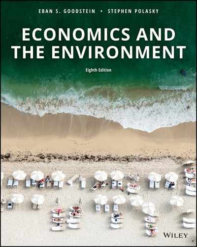
In contrast to the clunker program, RECLAIM is a textbook cap-and-trade system. In operation since 1993, the program requires about 330 stationary sources to hold (tradeable) permits for each ton of sulfur dioxide () and nitrogen oxide () emitted. Figure 16.1 illustrates both the number of allowances issued and the actual emissions by RECLAIM companies for during the first 12 years of the program. Note that the total number of allowances granted to firms shrunk every year up until 2003. The initial allocation of allowances was quite generous—well above historical pollution levels. It was not until 1998 and 1999 that actual reductions below pre-RECLAIM levels were required for and , respectively. (The high initial allowances were apparently a political concession to promote industry buy-in.)

FIGURE 16.1 Reported Emissions and Allowances under RECLAIM
Source: Luong, Tsai, and Sakar (2000); Harrison (2006) and Fowlie, Holland, and Mansur (2009).
The tremendous excess supply of permits led to a slow start for the permit market: in 1994 and 1995, many could not be sold even at a zero price. Moreover, although RECLAIM required continuous emissions monitoring and electronic reporting, it took a couple of years for monitors to be installed and certified at some firms. However, by the end of the decade, the monitoring bugs were mostly worked out, and the allowance constraints were beginning to bind. In fact, in 1998, 27 firms violated the regulations by polluting more than their permitted levels. As supply diminished, permit prices rose while trading accelerated; in 1999, 541 trades occurred, valued at $24 million.8
RECLAIM was severely tested during the California energy crisis of 2000–2001. At the same time that the number of allowances were shrinking, energy prices went through the roof, and existing California power plants began operating on overtime schedules. As a result, demand for permits in particular shot up, and prices rose almost tenfold—from $4,300 per ton in 1999 to around $39,000 per ton in 2000. (These higher prices for permits fed back into higher electricity prices.) During the crisis, emissions broke through the cap by about 6 percent (see Figure 16.1). As a result, California regulators fell back to CAC strategies, pulling power plants out of the RECLAIM program to stabilize emission prices.
After a 4-year hiatus, in which power producers were required to install technologies capable of reducing emissions by 90 percent, in 2005, the plants rejoined the trading program. RECLAIM scheduled an additional round of cuts in the allocations: 20 percent below the levels in 2004 as shown in Figure 16.1 by 2008. To guard against future price surges, California regulators now have the discretionary authority to issue additional permits if prices rise above $15,000 per ton, allowing pollution levels to rise up to 2004 levels in the following year.9
As with the clunker program, RECLAIM ignores hot-spot issues. This may pose little problem if and are regionally mixed. However, critics have argued that toxic co-pollutants may be associated with the criteria pollutants, so and hot spots may, in fact, also generate toxic hot spots.10
To recap the U.S. experience with trading urban air pollutants, the EPA’s early experiments were effective at promoting internal trades, but external trades were hampered by thin markets. Los Angeles’s clunker program has experienced both monitoring and hot-spot problems, and RECLAIM fell victim to unanticipated price volatility.
On a more optimistic note, the East Coast trading system got off to a good start. Initiated in 1999, the first round of trading included 11 states, and by 2002, large electrical generators and industrial boilers were trading credits equal to only 46 percent of their 1990 emissions. In 2005, the Bush administration federalized the trading program, expanding it to 25 states under the Clean Air Interstate Rule (CAIR). CAIR has since been challenged by price volatility, due to uncertainty over court challenges, and later the impact of climate regulation on emissions.11
16.3 Marketable Permits and Acid Rain
To date, the defining “grand experiment” with cap-and-trade in the United States has been the sulfur dioxide trading program designed to reduce acid rain. Acid rain is formed when sulfur dioxide, primarily released when coal is burned, and nitrogen oxide, emitted from any kind of fossil-fuel combustion, are transformed while in the atmosphere into sulfuric and nitric acids. These acids return to the earth with raindrops or, in some cases, as dry dust particles. Acid deposition directly harms fish and plant life and also can cause indirect damage by leaching and mobilizing harmful metals such as aluminum and lead out of soil. The impact of acid rain on ecosystem health varies from region to region, depending on the base rocks underlying the area. Naturally occurring limestone or other alkaline rocks can neutralize much of the direct impact of the acid. Such rocks are not found in the primarily igneous terrain of the Adirondack Mountains in New York state, southeastern Canada, or northern Europe, so damage to lakes in these regions has been extensive.
In addition to damaging water and forest resources, the acids erode buildings, bridges, and statues. Suspended sulfate particles can also dramatically reduce visibility. Finally, they contribute to sickness and premature death in humans.12
Pollution from sulfur dioxide was at one time concentrated around power plants and metal refineries. The area around Copper Hill, TN, for example, was so denuded of vegetation from now-closed copper-smelting operations that the underlying red clay soil of the region was clearly visible from outer space. In an attempt to deal with these local problems, and with the encouragement of the ambient standards mandated by the Clean Air Act of 1970, taller smokestacks were built. And yet, dilution proved not to be a pollution solution. Sulfur and nitric oxides were picked up by the wind and transported hundreds of miles, only to be redeposited as acid rain. The acid rain problem in the northeastern United States and Canada can thus be blamed on regional polluters—coal-fired utilities and nitrogen oxide emitters ranging from the Midwest to the Eastern seaboard. Similarly, Germany’s forest death and acidified lakes in Sweden and Norway required a Europe-wide solution.
Increasing environmental concerns, along with the large health risks from sulfate pollution discussed earlier, finally led to action on acid rain by the 1990 Clean Air Act. The legislation created the SO2 trading system, requiring a 10-million-ton reduction of sulfur dioxide emissions from levels in 1980, down to an annual average of 8.95 million tons per year, and a 2.5-million-ton reduction of nitrogen oxide emissions by 2000.13
The first stage of the rollback was achieved in 1995 by issuing a first round of marketable permits to 110 of the nation’s largest coal-burning utilities, mostly in the East and Midwest; the second stage, begun in 2000, imposed tighter restrictions and included another 2,400 sources owned by 1,000 other power companies in the country. To reduce the financial burden on, and political opposition from, utilities and ratepayers, most of the permits are not sold by the government. Instead, utilities are simply given permits based on their emission levels in 1986. Each utility receives permits equivalent to 30–50 percent of its pollution level in 1986.14
Trading is nationwide, although state legislators and utility regulators do have the authority to restrict permit sales. Given such a broad market, a utility in, say, Ohio has little power to prevent a competitor from setting up shop in the neighborhood merely by refusing to sell permits. Such a firm could simply go shopping in Texas. Finally, to safeguard against potential market power problems arising if new entrants are forced to buy permits from incumbent competitors, the government distributes 2.8 percent of the permits by auction and sale.
Because sulfur dioxide and nitrogen oxides emitted from the tall stacks of power plants are more or less uniformly mixed on a regional basis (and because midwestern plants are net sellers), major geographical hot spots have not emerged from the acid rain program.15
The program created an 8.9-million-ton cap on emissions from power plants after 2000. However, Congress has the authority to reduce the number of permits even further without buying them back from the firms. The states’ authority to impose tighter regulations has also not been affected. Thus, the permits confer no tangible property rights, although firms certainly expected at least a decade’s trading before the emission cap was reconsidered.
On the enforcement front, the acid rain program mandated the installation of continuous monitoring equipment, which is required to be operative 90 percent of the time and to be accurate to within 10–15 percent of a benchmark technology. The EPA certifies the monitors at each plant; thus, the monitoring process itself retains the CAC features. Once a plant’s monitoring units are certified, the EPA records all trades and then checks allowances against emissions on an annual basis to ensure compliance.
Violators face a $2,000-per-ton fine for excess emissions and must offset those emissions the following year. The fine level was set substantially above the expected market price and yet not so high as to be unenforceable. Thus, it represents a very credible threat to firms. In addition, once a violation is established, the fine is nondiscretionary. These factors have led to very high compliance rates.
As a last note, the acid rain legislation contained measures to compensate high-sulfur coal miners and others who lost their jobs. Funding for support while in job-retraining programs was authorized at a level of up to $50 million for 5 years. Job-loss estimates through the late 1990s were on the order of 7,000 in total, almost all of them being eastern coal miners.16
Before the program was introduced, economists were optimistic that the legislated acid rain trading program, expected to cost about $4 billion annually, would result in savings of between 15 percent and 25 percent over a stereotypical CAC option.17 This optimism arose because the theoretical objections to an IB approach raised in the previous chapter, some of which contributed to the disappointing performance of bubbles, did not appear likely to emerge in this case.
To begin with, the existence of a national market with hundreds of participants (including the Chicago Board of Trade) minimizes transaction costs and the thin market problem. Because of the approximately uniformly mixed nature of the pollutants, major hot spots were unlikely to emerge. The potential exercise of market power and speculative behavior was mitigated by the set-aside and auction of a limited number of permits. The issue of permit life was settled by providing firms with an indefinite guarantee—a cap of 8.9 million tons in 2000 with Congress holding the authority to restrict emissions further. And finally, an up-front commitment to better monitoring technology and streamlined enforcement was made.
From an economic point of view, the acid rain program was one of the best-laid regulatory plans. Nevertheless, to paraphrase Shakespeare, reality often reveals more complications than are dreamt of in our philosophy. This experiment has been worth monitoring closely as it unfolds; the results to date have been quite positive.
First, both and emissions from the power plants participating in the program have fallen sharply since 1995. Ambient (airborne) levels of sulfur dioxide have declined as well. This decline has been linked to both improvements in visibility in national parks and significant health benefits—reductions in both sickness and premature death. Based largely on these health benefits, the acid rain program easily passes an efficiency test; the measurable benefits of the acid rain program far exceed the costs.18
The big positive surprise from the program has been the dramatic cost savings: utilities achieved the cutbacks by spending less than one quarter of what the cap-and-trade system was originally predicted to cost, which in turn was well below the forecast costs for a traditional CAC system. Before the program went into effect, the EPA estimated that compliance costs for the cap-and-trade system would be $4 billion annually; that estimate has now fallen to less than $1 billion. Most analysts thought that marginal control costs (and thus permit prices) for would settle in at between $750 and $1,500 per ton. Instead, for the first few years of the program, permits sold for between $100 and $150 per ton, though they have climbed as high as $700 per ton.19
During the first 2 years of the program, relatively few trades between different firms actually occurred; in 1995, less than 5 percent of the permits in circulation traded hands. Both the phenomena of dramatically lower costs and fewer-than-expected trades can be explained in retrospect by the increased flexibility that firms were given under the acid rain program. Rather than installing expensive scrubbers (or buy extra permits), most firms met their early targets by switching to low-sulfur coal or developing new fuel-blending techniques. Railroad deregulation led to an unexpected decline in low-sulfur coal prices. And with the increased competition from coal, scrubber prices fell by half from 1990 to 1995.
Recall that a stereotypical CAC regulation has two features that raise costs: uniform standards (which block short-run cost-reducing trades) and technology-based regulations (which discourage long-run cost savings by restricting firm-level compliance options). In the acid rain case, almost all of the initial cost savings came from increased flexibility within the individual firm. This included the ability to engage in intrafirm trading (so that any single firm’s different plants don’t face uniform standards) as well as the ability to use a mix of control technologies.
However, as Figure 16.2 illustrates, interfirm trading picked up dramatically after year 3. Environmental managers at utilities took a while to exhaust internal cost savings from trade and then began to look outward.20 Thus, even greater cost savings emerged as interfirm trading accelerated. All in all, the acid rain program is a case where economic theory has done a very good job guiding government policy. Emissions have been reduced at low cost and with a high degree of certainty.
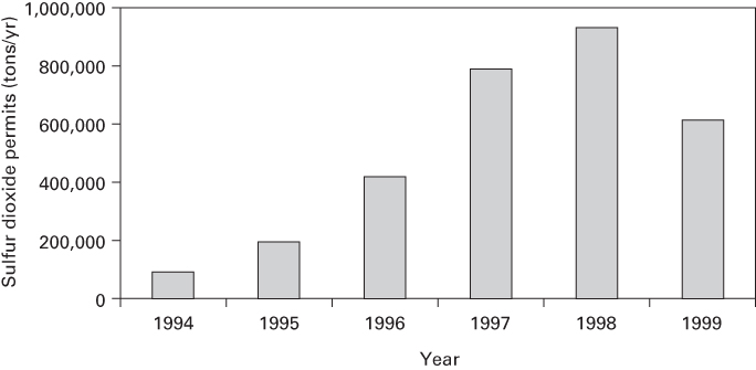
FIGURE 16.2 Interfirm Permit Trade under the Acid Rain Program
Source: U.S. EPA Acid Rain Program, www.epa.gov/docs/acidrain.ats/qlyupd.html.
16.4 Carbon Trading in the Northeast and California
In 2005, seven Northeastern U.S. governors signed on to the Regional Greenhouse Gas Initiative, better known as RGGI. In the absence of any federal controls on global warming pollutants, these states decided to act on their own, agreeing to stabilize carbon dioxide emissions from the electric power sector at projected levels in 2009 and then reduce by 10 percent from there through 2018. From a short-run efficiency perspective, this effort makes no sense. State residents will bear some costs for the reduction, primarily in the form of higher electricity prices, and because the emission reductions proposed are so small relative to world emissions, the effort on its own will have no noticeable impact on future global temperatures. Why do it, then?
One reason was to provide leadership in an attempt to overcome the free-rider problem; the states hoped to set an example that the U.S. federal government would soon follow. And under the assumption that this would eventually happen, Northeast states hoped to then capitalize on technology leadership established as they began to reshape their economies to rely less on inputs of fossil fuels. In addition, by reducing the use of out-of-state coal, and investing permit proceeds in weatherizing homes and other energy-efficiency measures, the states hoped to keep more of their energy dollars at home, boosting in-region growth.
RGGI trading began at an unfortunate moment: in late 2008, just as the economy was sliding into a recession. Due to sluggish economic growth and also the unexpected surge in natural gas generation at the expense of coal (see Chapter 18), by 2012, carbon emissions from the region were already 30 percent below the initial cap. Thus, RGGI permits have been trading at very low prices, around $2 per ton, with many of the auctioned permits going unsold. In 2012, regulators tightened the cap.21
Even as initially envisioned, RGGI would not have cost individual consumers much, because the emission cuts it proposed were relatively small. By 2015, RGGI was expected to raise electricity prices by around 1 percent or less, with annual costs ranging from $3 to $16 per family. As auction revenues from the program are used to invest in energy-efficiency measures, net energy payments by many New England residents might actually decline. Much of the policy discussion around RGGI has been devoted to this issue of permit sales revenues. First, how much money is at stake? Second, how many permits should be given away and how many auctioned? Third, what should be done with the auction revenues?
Although not a lot of money for an individual household, the total auction revenues that RGGI generates are large: by 2013, over $2 billion. After significant debate, the RGGI states now auction 90 percent of the total permits. States are using RGGI dollars to fund energy-efficiency measures, to fund renewable energy, to assist low-income consumers with electricity bills, and in some cases, to cover general expenses. One study has argued that, on net, these recycled revenue dollars have indeed boosted the regional economy.22
Finally, an interesting feature of RGGI is that it allows electricity producers to achieve some of their mandated reduction in carbon dioxide via the purchase of offsets—reductions in greenhouse gasses achieved offsite by third parties and then packaged and sold. RGGI specifically allows offsets from the following sources:
- Natural gas, heating oil, and propane energy efficiency
- Landfill gas capture and combustion
- Methane capture from animal operations
- Forestation of nonforested land
- Reductions in sulfur hexafluoride emissions from electricity transmission and distribution equipment
- Reductions in fugitive emissions from natural gas transmission and distribution systems
Offsets from non-RGGI states are allowed, but at a 1-ton credit for each 2 tons of verified reductions.23
Since around 2000, offsets have also been available for purchase by companies and individuals not required to reduce their emissions. Several nonprofit organizations around the country offer individual consumers the opportunity to voluntarily offset their personal carbon dioxide emissions and become “carbon neutral” or “carbon cool.” (See www.carboncounter.org, for example.) In 2003–2004, the school where one of us used to teach, Lewis and Clark College, became the only school in the world to be (temporarily) compliant with the Kyoto treaty through the purchase of $17,000 of offsets; the money was voted out of student fees, at about $10 per student. The student funds helped to support new wind-power development in Oregon, among other projects.
The offset market has grown up around voluntary initiatives to reduce greenhouse gases; initiatives such as RGGI will help this market grow. A serious problem with offsets is quality control. In particular, to have real value, offset projects must be additional. This means that the project—reforestation, reduction in fugitive emissions from pipelines—would not have already occurred under a business-as-usual scenario.
With the RGGI experiment, large-scale carbon trading got under way in the United States in 2009, years before trading was likely to kick in across the nation. California is now following the Northeast, with a more ambitious economy-wide cap-and-trade initiative that was launched in 2013. If California were a nation, it would be the eighth biggest greenhouse gas emitter in the world, so the effort is internationally significant.
California’s program, known as AB32 for the law that created it, requires that the state economy roll back greenhouse gas emissions to 1990 levels by 2020. This is a 22 percent reduction compared to forecasts of what business-as-usual emissions would be. Most of this reduction will not actually be driven by cap-and-trade, but rather by complementary policies (discussed in Chapters 17 and 18) including a renewable portfolio standard for the electricity sector, a clean-car mandate, a low-carbon fuel standard, and the million solar roofs program. The trading system is designed to achieve about 30 percent of the total reductions.24
Starting in 2013, around 450 electricity generating plants (including plants that import electricity into California) and large industrial facilities faced carbon caps. In 2015, another 100 distributors of transportation fuels and natural gas came into the system. Together, these facilities account for about 85 percent of total California greenhouse gas emissions. Each year, the total number of permits that will be available to these businesses will decline, reaching the 1990 levels by 2020.
Industrial facilities started out with free allowances to provide them time to adjust to lower emissions and also to protect trade-exposed industries. Other sectors must purchase permits at auction. By 2015, about 50 percent of the permits were sold by the state, raising over $2 billion in revenue. By California law, any revenues generated through fees—such as permit auctions—must be used to further the purpose of the fees, in this case, greenhouse gas reduction. Auction revenues raised in the utility sector must be used to benefit rate-payers—through measures such as rebates on their bills, energy-efficiency investments, or renewable investments.
There is currently a robust debate underway in California as to what to do with the remaining revenue. The money might be rebated back to households, “skytrust” style; invested in high-speed rail connections between San Francisco and Los Angeles; used to support renewable or efficiency investments; or used in any of a variety of other options consistent with the goal of equitably cutting greenhouse gas emissions. Whether those funds are invested productively will be key to both the economic impact of the law in California and the state’s ability to meet deeper emission reductions it might pursue post-2020.
Firms can meet up to 8 percent of their pollution limit through the use of offsets, which must be “permanent, verifiable, enforceable” and, of course, additional. Offsets must be certified through third-party, employ-approved protocols and are currently limited to the United States.
The program has a price collar, with a floor of $10 per ton, and a set of ceiling triggers at $40, $45, and $50 in 2012, rising at 5 percent each year plus inflation. To keep prices below the triggers, the state is authorized to issue up to 4 percent additional permits at each trigger point, for a total increase in supply of up to 12 percent. There is unlimited banking, and compliance is measured over a 3-year average period. Firms pay a fine for noncompliance, by being required to purchase four additional tons for every ton for which they are over their limit.
California’s AB32 system is benefiting from 25 years of experience with cap-and-trade systems. By moving quickly to an auction system, the state is avoiding the problem of windfall profits accruing to producers (see Chapter 15, Section 15.4) while still providing some period for adjustment; offsets are limited and regulated to ensure high quality; and the price collar is designed to protect the system from the price volatility at both ends that has plagued other programs. In addition, the legal mandate requiring that auction revenues be used to further the purposes of the program may help ensure productive investment of auction proceeds—the resource rent generated by restricting access to common property.
The California system faced a serious political challenge on the 2010 ballot, when two Texas oil companies funded an initiative that would have repealed the law. California voters were treated to a rare TV ad war: “cap-and-trade will kill jobs” said one side; “cap-and-trade is creating jobs in a clean energy economy” said the other. At the end of the day, AB32 was reaffirmed by the voters 2–1.
16.5 Two Failed U.S. Efforts: Mercury and Carbon
Two major federal cap-and-trade systems were proposed but did not advance during the 2000s, and the reasons for their failure are instructive. During the George W. Bush presidency, the United States tried to launch a trading system for mercury emissions from coal plants. Airborne mercury from fossil-fuel combustion winds up in lakes, rivers, and oceans, where it bioaccumulates in fish. Through this and other exposure routes, perhaps 10–20 percent of pregnant women in the United States have elevated mercury levels; the figure doubles for Native American and Asian American women. Not all of this contamination comes from U.S. emissions; ocean deposition primarily from coal plant emissions and contamination of fisheries are a global, transboundary problem.
Mercury originally escaped regulation under the original Clean Air Act. It was categorized as a hazardous pollutant or air toxic, not a criteria pollutant, and thus fell prey to regulatory gridlock discussed in Chapter 13. Following the air toxics mandate of the 1990 CAA amendments, in 2000, the Clinton EPA finally announced its intent to impose maximum achievable control technology (MACT) requirements for mercury, a CAC regulatory approach that would have required emission reductions at all sources on the order of 90 percent by 2009. The Bush administration EPA, however, did not follow through on this finding. Instead, in 2005, the EPA recategorized mercury as a criteria pollutant and announced plans for a mercury cap-and-trade program designed to reduce emissions by 20 percent by 2010 and 70 percent by 2018. The reductions up to 2010 were anticipated as “co-benefits” resulting from existing and regulations and would not have imposed additional costs on industry.
Efficiency and safety advocates sparred over the very different stringency levels recommended by the Bush and Clinton EPAs. But the particular issue of interest here is the question on hot spots: is this a case in which a CAC uniform emission reduction requirement is needed or will trading be acceptable? The Bush EPA argued that no hot spots would emerge from the proposed trading program. Yet, many analysts were not convinced: local and regional hot spots appeared possible in the upper Great Lakes states of Michigan, Minnesota, and Wisconsin, potentially imposing high costs on rural and Native American populations.
Because of concerns about both hot spots and pollution levels, the Obama administration scrapped the Bush plan and returned to regulating mercury emissions as air toxics, using a CAC approach such as that proposed by the Clinton EPA. In 2013, more than 40 years after the original passage of the Clean Air Act, mercury emissions finally came under EPA regulations.25
Beyond mercury, the Obama administration also supported its own, ultimately unsuccessful national cap-and-trade system, this one for global warming pollutants, primarily carbon dioxide. The system would have been authorized by the American Clean Energy and Security Act (the Waxman–Markey Bill), which passed the House of Representatives in June 2009. However, the Senate was unable to pass a comparable bill, and with the 2010 elections and the rise of Tea Party politics, the political coalition supporting cap-and-trade collapsed.
The House Bill is worth examining because of the way it tried to solve key obstacles: the law sought to insulate residential consumers from price increases and also controlled costs through generous offset provisions. The bill proposed a goal of reducing global warming pollutant emissions from fossil-fuel combustion of 17 percent below the levels in 2006 by 2020 and 80 percent by 2050. Covered sectors include electricity producers, oil refineries, natural gas suppliers, and energy-intensive industries: steel, cement, chemical, and paper manufacturers. Combined, these sectors account for 85 percent of economic activity.
Around 75 percent of the permits would have been given away to polluters, based on their past emissions of global warming pollutants; 10 percent given to states to be sold for efficiency, renewables, and other investments; and 15 percent auctioned by the federal government. Beginning in 2025, giveaways to industry would be phased out, and the program would have moved toward 100 percent auction by about 2030. Note that relative to RGGI and California’s AB32, the proposed federal program was much more generous to industry and, for many business sectors, would actually have provided windfall profits (as discussed in Chapter 15). This reflected the weakness of the political coalition supporting cap-and-trade at the national level and the need for greater industry buy-in.
Around 5–10 percent of the federal government revenue would be used to help developing countries cut deforestation and implement clean technology solutions. In addition, the bill mandated that a big chunk of government auction revenues—rising over time—would go to weatherization and other efforts to reduce household energy consumption. Finally, as in California, the value of permits given to regulated electric power distributors was required to be passed on to consumers in the form of rebates or other measures.
These kinds of conservation and efficiency efforts were predicted to have a major effect. The EPA estimated that demand would be cut so far that “energy consumption levels that would otherwise be reached in 2015 without the policy are not reached until 2040 with the policy.” Overall—through this demand reduction and the mandated rebates to households from their utilities—the EPA believed that households would largely be shielded from increases in their monthly payments for electric power.
Finally, very generous offset provisions also contained the estimated overall cost of the program. The House bill allowed up to 2 billion tons of offsets per year with the possibility of more than 50 percent of these being international. This number was large: currently, around 30 percent of total emissions. But, the relative size of this offset pool would have grown in importance over time, as U.S. domestic emissions shrank. By 2050, this 2 billion tons of offsets—if fully utilized every year—would have meant that instead of “real” emission reductions of 80 percent by companies, U.S. producers would have cut only 60 percent.
The availability of international offsets in particular, and especially in the later, “deep cut” years of the program, reduced expected prices a lot—by close to 90 percent. Why is this so important? It would be much cheaper to clean up inefficient, dirty coal plants in India, or to plant new forests in Ecuador, than it would be to squeeze an additional 20 percent out of the U.S. economy, for example, by shutting down the remaining coal-fired power plants or converting them to biomass. At the same time, of course, these offsets would also be much difficult to monitor, and they raised real concerns about the possibility of fraud.
Finally, transition assistance would have been provided in the form of free allocation of permits to energy-intensive and/or trade-exposed industries. As in California, these firms could use the “windfall profits” from their free permits to cushion the increased compliance costs, and any international competitive disadvantage, that they might face. (Unlike California, however, the U.S. system proposed continuing the permit giveaway program to all firms for more than a dozen years.) Workers in heavily affected sectors—certainly in coal mining, and potentially in rail shipping of coal—would have access to extended unemployment benefits and support for health-care payments (up to 3 years), job-search expenses, and some relocation allowances.26
As noted, support for the cap-and-trade bill disappeared after the 2010 elections. And Tea Party opposition to national global warming legislation means that a national cap-and-trade program (or a carbon tax) is likely off the table for the next few years. Nevertheless, with high probability, the world will continue to heat up. As a result, political support for national action on climate change will undoubtedly resurface. At that point, analysts will look back to Waxman–Markey for guidance.
In the meantime, as noted earlier and in Chapter 13, carbon dioxide is being regulated through state and regional cap-and-trade systems, and nationally under the Clean Air Act, with the EPA pursuing the CAC strategies for stationary and mobile sources that are enabled by that legislation. And elsewhere in the world, China and Korea are moving ahead with their own plans for carbon cap-and-trade systems.
16.6 The European Emissions Trading System
Europe is far ahead of the United States, having kicked off a comprehensive carbon cap-and-trade system in 2005. European nations all ratified the 1997 Kyoto treaty, which required reductions of global warming pollution level in Europe to about 7 percent below the levels in 1990 between 2010 and 2012. In anticipation of the treaty going into force, the EU established the European Trading System (ETS). Under the Kyoto treaty, each country has a carbon cap, and each country must develop an implementation plan to achieve the required emission reductions. Typically, the nationwide caps are translated into sector- or firm-specific caps. The ETS then allows continent-wide trading of carbon between companies, so that companies (and countries) that have a hard time making their mandated targets can purchase excess emission reduction credits from companies that have beaten their targets. The ETS covers over 12,000 major emitters from the power sector—oil refiners, cement producers, iron and steel manufacturers, glass and ceramics, and paper and pulp producers, accounting for about 40 percent of Europe’s global warming pollutant emissions.27
Since its initiation, the ETS has updated its target—now 21 percent below the levels in 2005 by 2020—and has modified some of its rules. Of the 15 western European countries, by 2009, 5 countries—The United Kingdom, Germany, Sweden, France, and Greece—were below their Kyoto targets. With the global recession and a sluggish economy since 2008, the EU actually met its 2020 target in 2014, 6 years early! The ETS cap now effectively acts as a break to ensure that emissions do not rise above the cap over the next few years. Finally, in 2013, the ETS also included aviation emissions under the cap—the first time this major source of global warming pollution had fallen under a regulatory system.28
Challenges to the system have included problems of price volatility and concerns about offset provisions. Trading in Europe commenced in 2005, and prices for the first year rose from 15 to 30 euros per tonne of . But, over the next 2 years, the market was subsequently shaken by two periods of sharp price declines and then recovery, reflecting changes in policy, and then experienced a sustained collapse in prices during the great recession of 2008, Europe’s slow recovery since 2008, combined with the growth of renewable power, has in fact kept emissions well within the ETS cap, even as it has declined. The excess supply of carbon permits has kept prices low. Note that the “price stability problem” in Europe is the opposite of what occurred in Los Angeles: not excessive prices, but instead, repeated periods of prices so low that firms had little incentive to undertake long-run investments in emission reductions. There is also concern that, because so many permits have been banked—purchased but not used—prices will take a long time to recover.29 The European experience speaks to the need not only for a price ceiling but also for a price floor.
In addition to trading within Europe, the Kyoto treaty and the ETS allow companies to meet their targets via offset purchases from developing countries that do not face caps under the accords. The so-called Clean Development Mechanism (CDM) allows, for example, a German electric power company to gain credit for carbon dioxide reductions by replacing a proposed coal power plant in India with a new wind farm. Here again concerns have been raised about the quality of these offsets and ensuring that they are indeed additional. Reforestation efforts in particular raise quality issues: how will investors be assured that the trees will not later be harvested—or even burn down? Third-party certifiers and government oversight mechanisms have begun to arise as an attempt to ensure both additionality and quality.30
In addition to price volatility, the ETS has been criticized because all the permits were initially given away to industry, and few attempts were made to protect consumers from higher prices for “dirty” (-intensive) goods such as gasoline. With the permit giveaways came windfall profits for some producers, who received these valuable permits at no cost and then sold them. As a result, since 2013, at least 50% of the permits must be auctioned by member states.31
The ETS experiment—featuring an international cap-and-trade system with the CDM offset market thrown in—is by far the most ambitious pollution-control system ever put in place. Given its complexity, some economists and other observers are concerned that the European Trading System may ultimately falter on the critical monitoring and enforcement front. The current challenge, as with RGGI, is how to sustain prices when, due to economic conditions, emissions unexpectedly fall well below the cap.
To summarize on carbon cap-and-trade, over the last few years, some U.S. states and Europe have taken initial, significant steps toward 80 percent by 2050 reduction. If these policies are effective, and if following the Paris Climate Agreement the rest of the world goes along, these efforts will hold the thickness of the carbon blanket to between 450 and 650 ppm. If we stabilize at the low end of 450 ppm, this, in turn, provides some assurance (about a 30 percent chance, according to the Stern Review) that global temperatures will not rise by more than 4 degrees F.32 To get to the low end will require more and more regions to adopt aggressive carbon caps or other measures like carbon fees.
16.7 Pollution Taxes and Their Relatives
In contrast to numerous global applications of cap-and-trade, pollution taxes are relatively rare and are emerging primarily to attack global warming. A textbook example is found in British Columbia. Since 2008, residents there have been paying a levy of $30 per ton—which adds about $0.10 to a gallon of gasoline. When the tax was instituted, the government gave each household a lump-sum rebate of $85 and cut a number of other taxes to ensure that the policy was “revenue neutral.” Despite these measures, the carbon tax became a major issue in the 2009 provincial elections, but—this time, going against the general trend—the public actually endorsed the tax, returning its political architect back into office. Other Canadian provinces are expected to adopt taxes of cap-and-trade systems within the next few years. Other countries that have instituted carbon taxes (or close relatives) include Sweden, Norway, Britain, and The Netherlands. Carbon prices have been a political football in Australia in recent years. A tax of $24 per ton of carbon that went into effect in 2012, paid initially by the biggest few hundred businesses and government entities, was later repealed.
In the United States, there are a number of price policies in place that affect the environment, though no real pollution taxes: fees levied per pound, liter, or ton of pollutant emissions. In this section, we examine several of these incentive instruments and also look at “indirect” pollution taxes—energy taxes—in Europe. We will start with waste disposal fees.
Homeowners typically pay by the gallon for sewage disposal, and waste haulers pay by the ton to dispose of hazardous and solid waste. These closely resemble textbook pollution fees, which in theory should result in conservation measures as disposal costs rise.
However, at least in the case of solid waste, this has not been the general result because the incentives for waste reduction are not always passed on to consumers. Historically, much residential, commercial, and industrial municipal solid waste disposal is financed through a lump-sum fee. Thus, residential consumers may pay, say, $10 per week for garbage service regardless of how much garbage they produce. In some communities, city government handles waste disposal, and the fee is included in property taxes; in others, private firms charge for disposal on a weekly or monthly basis.
This presents us with a curious problem:
In the past, solid waste disposal fees have been relatively low. However, as landfills around the country close and political resistance to new construction has arisen, solid waste disposal costs have been rising rapidly. This has led an increasing number of municipalities to switch to unit pricing, often in combination with curbside recycling programs, as a way to reduce waste flows.34
In a study of unit pricing in suburban Perkasie, PA, semirural Ilion, NY, and urban Seattle, Washington, the introduction of unit pricing in the first two communities reduced waste actually generated by 10 percent or more, while the flow to the landfill was reduced by more than 30 percent. In addition, these two communities reduced their waste management costs by 10 percent or more and passed on the savings to households through reduced fees. At the same time, unit pricing was adopted, both of these communities also introduced or expanded curbside recycling.
By contrast, Seattle’s unit-pricing program was evaluated before the introduction of curbside recycling. Seattle had a unit-pricing system in place since 1961 but substantially raised the rates per can over the 3 years of the study. The response among Seattle residents to the rising rates was to increase trash compaction (locals call it the “Seattle Stomp”), slightly increase the recycling rates, and, ultimately, slightly reduce the overall waste generated. The study suggests that, in the absence of a good substitute (curbside recycling), waste disposal is fairly insensitive to price increases; that is, it is price inelastic.
Of course, a pollution tax will always drive people to look for unintended substitutes. In the Perkasie case, the shift to unit pricing led to an increase in trash burning, which was subsequently banned, and to an increase in out-of-town disposal. However, the town found no increase in sewage disposal of waste. Seattle reported some increase in illegal dumping.35
Unit pricing for garbage disposal is about as close as we get to a pollution tax in the United States. However, a variety of other fee-based approaches, while also not classic Pigovian taxes, are in use.
USER FEES FOR PUBLIC LANDS AND ROADS
Hikers, recreational fishers, hunters, logging companies, and ranchers must all pay the federal government permit fees for the use of public resources. Many have argued that some or all of these fees are much too low to discourage overexploitation. Nevertheless, they represent a mechanism by which common property resources are priced and by which marginal damages can, at least in theory, be controlled.
What external costs do hikers impose? Too many hikers can damage trails, and of course, hikers generate congestion externalities—the last hiker crowding the trail reduces the value of the day’s hike for all the previous users. Economists have recommended fees as an important component of a land manager’s toolbox for rationing access to scarce trails. Similarly, congestion pricing on highways is an economically efficient—though seldom used—way out of urban traffic jams.
ENVIRONMENTAL BONDS
As discussed in Chapter 8, deposit requirements for beverage containers and automobile batteries and bonds posted by strip mines or landfill owners are ways to internalize the social cost of “irresponsible” disposal or development.
INSURANCE AND LIABILITY REQUIREMENTS
Under the Oil Pollution Act, oil tankers entering U.S. waters must show proof of insurance of around $1,200 per gross ton of cargo. An insurance requirement of this type is similar to an environmental bond, and if insurers charge higher rates for tanker operators with riskier histories, insurance markets act to help internalize the social costs of risky behavior. (In the tanker insurance market, in fact, insurance rates do go up for carriers that have more oil spills, but probably not at a rate sufficient to fully internalize the environmental damage costs.)36
Damage insurance is critical to internalize the environmental costs for businesses likely to suffer low-probability but high-impact accidents. In this regard, the nuclear power industry has long held on to a critical but hidden governmental subsidy. Because nuclear plants would otherwise be unable to obtain private insurance, the Price–Anderson Act limits liability for nuclear accidents. On a per-reactor basis, the subsidy works out to be more than $20 million dollars per year.37 By shielding the nuclear industry from this cost of operation, the Price–Anderson Act encourages the growth of nuclear power beyond what the market would support.
ENERGY TAXES
Energy taxes can serve as indirect pollution taxes. Europe has a long history of high fossil-fuel taxes designed to both reduce pollution and improve energy security.
Two weeks before writing this section, I, Eban, returned from a trip to Denmark, where I visited my cousins. They had borrowed a friend’s house for us to stay in, and when we departed, my cousins left a little envelope with some money in it “to pay for the electricity,” they said. This was a little surprising to me, because in America, we are used to thinking of electricity as a virtually free good. But, due to high taxes on energy, Danes pay more than twice as much as we do for electricity. As a result, they think about their energy use more carefully than we do.
The production of energy via the burning of carbon-based fuels is a highly polluting process. Most of the criteria air pollutants are generated this way, while upstream mining of oil and coal results in destruction of sensitive habitat and in acid mine pollution. As Table 16.1 shows, for uncontrolled pollutants such as carbon dioxide, the relationship between energy use and pollution is fairly clear-cut. The United States, with its high per-capita energy use, also has the highest per-capita carbon dioxide emissions. The table also shows a strong negative relationship between energy prices and energy consumption. High prices promote low consumption, and vice versa. Thus, one strategy to reduce pollution is to tax it indirectly by taxing energy use.
TABLE 16.1 Energy Consumption, Prices, and CO2 Emissions
Source: World Resources Institute Energy consumption data are from 2003, World Resources Institute; data are from 2006, U.S. Department of Energy’s Carbon Dioxide Information Analysis Center (CDIAC); gasoline price data are from Randall, Tom (2013) “Highest & Cheapest Gas Prices by Country”, Bloomberg, 2/13/13 http://www.bloomberg.com/slideshow/2013-02-13/highest-cheapest-gas-prices-by-country.
| Country | Energy Consumption per Capita (kg of oil equiv.) | CO2 Emissions per Capita (tons) | Gasoline Price ($/gallon) |
| US | 7794 | 19 | 3.29 |
| Japan | 4040 | 10 | 6.70 |
| Germany | 4203 | 10 | 7.96 |
Indeed, since the late 1990s, Great Britain has imposed an energy tax called the Climate Change Levy. It is not, strictly speaking, a global warming pollution tax, as it taxes energy produced, not carbon emissions. Yet, by exempting renewable power production—and rebating some of the levy revenues to clean power producers—the levy does provide some incentives to help meet Britain’s Kyoto targets. (The remainder of the revenues are rebated to power producers in the form of an across-the-board cut in payroll taxes.) Recently, the Conservative Party candidate in Britain’s election was calling for the replacement of the levy with a bona fide carbon tax. Why? By taxing energy instead of carbon emissions, the levy leaves some firms with large bills, regardless of whether they are reducing their carbon footprint. Also, the levy puts the whole burden of energy reduction on power producers—exempting the household and transport sectors, where emissions are rapidly increasing and could be reduced at the lowest cost.
The potential for these kinds of unintended “perverse effects” means that a direct pollution tax (a charge per ton of carbon) would clearly be preferred to an indirect energy tax (levied on the energy content of fuels), because the former taxes all sources on the basis of their pollution contribution and promotes a search for all types of cleaner energy sources. Nevertheless, energy taxes do have the advantage of being administratively simpler, particularly if there is no easy formula for assigning pollutant emissions to energy sources.
16.8 Summary
This chapter has reviewed our experience with incentive-based regulation. Cap-and-trade systems can work very well, achieving clear environmental goals with large cost savings ( trading for acid rain). Or, they can fail to achieve much of anything at all (the EPA bubble program). A primary lesson from the existing marketable permit systems is that a permit market can be a delicate thing. In markets with only a few players, potential traders are discouraged from participating, thus prolonging thin market problems. And as the L.A. Basin RGGI and ETS cases illustrate, price volatility has posed an unexpected and thorny problem.
Our experience with hot spots suggests that for nonuniformly mixed pollutants, permit designers face a trade-off between ensuring uniform pollution exposure and achieving a workable permit system. In practice, some compromise on safety has occurred (with the L.A. clunker system) for a permit system to be successfully implemented. For this reason, the proposed cap-and-trade system for mercury in the United States was highly controversial.
In recent permit systems, the choice between auctioning permits and giving them away free to industry has been an important decision. The trend is toward auction, with an initial giveaway period to support industry adjustment and to protect trade-exposed industries. Auction revenues can then be devoted to protecting consumers from price increases, through rebates and energy-efficiency investments as we have seen with RGGI and anticipate with California’s AB32.
Another recent development has been the “politicization” of cap-and-trade. Support for cap-and-trade was initially widely bipartisan. It was seen as a market-friendly alternative to CAC regulation. Acid rain permit trading in 1990 was supported by the first President Bush, and RGGI was supported by a bipartisan coalition of governors (including then Massachusetts Governor Mitt Romney); John McCain, the 2008 Republican presidential candidate, was a primary Senate cosponsor of several mid-2000 U.S. carbon cap-and-trade bills; and the California cap-and-trade legislation was championed by Republican Governor Schwarzenegger.
This changed in the 2010 election, with the rise of Tea Party politics and a tide of blanket Republican opposition—including that by candidate Romney—to all forms of cap-and-trade as a form of unwarranted taxation. Ironically, this has meant that U.S. national carbon policy has fallen back on CAC regulation under the Clean Air Act. For the next few years, the lack of bipartisan support for cap-and-trade renders unlikely any additional national experiments in this form of regulation.
On the pollution tax side, the main lesson to be learned from our experience is that they are very difficult to implement at levels high enough to function as a sole means of pollution control. Thus, taxes and other fee-based mechanisms should be viewed as a complement to, not a substitute for, conventional CAC regulation.
Finally, indirect pollution taxes such as gasoline or energy taxes are often a compromise solution when direct pollution taxes prove to be politically unfeasible or are too difficult to administer. In Europe and Japan, high energy taxes, originally imposed as energy security measures, have also functioned to reduce pollution levels in those countries, and Britain has imposed a specific Climate Change Levy, which is an indirect pollution tax on energy production.
Any type of regulation requires a strong commitment to monitoring and enforcement to be effective. This is especially true of IB regulation, where no special technology is mandated. In the U.S. context, two established marketable permit initiatives (acid rain and the RECLAIM program in Los Angeles) have featured an up-front commitment to better monitoring. However, some economists are concerned that the international complexity of the European Trading System for carbon dioxide (along with the offset option in the CDM) may be setting the system up to fail. The U.S. regional and state carbon cap-and-trade systems also need to confront these issues. If carbon trades are not carefully monitored and enforced, the credibility of proposals for future trading systems will be jeopardized.
KEY IDEAS IN EACH SECTION
- 16.0 This chapter discusses several real-world applications of incentive-based regulation: marketable permits and direct and indirect pollution taxes.
- 16.1 An early successful example of a marketable permit system was the lead banking program, because none of the obstacles identified in the previous chapter proved to be significant. A similar trading scheme also worked for ozone-depleting CFCs.
- 16.2 In contrast to the lead case, efforts to restrict other criteria urban air pollutants have had mixed success. The Emissions Trading Program has been disappointing relative to initial expectations. Emission reduction credits for criteria air pollutants are traded in the offset netting and bubble programs. Bubbles, in particular, have performed poorly because of thin markets and high transaction costs for nonuniformly mixed pollutants. Hot spots have largely been ignored in California’s RECLAIM and mobile source (“clunker”) trading programs. RECLAIM broke down temporarily under the pressure of the California energy crisis. By contrast, the East Coast NOx trading system seems to be off to a good start.
- 16.3 The biggest cap-and-trade success story is the national trading system, designed to reduce acid rain. This carefully monitored program achieved its pollution-reduction target and delivered substantial cost savings. Costs were reduced first as firms changed from installing scrubbers to burning low-sulfur coal, scrubber prices declined as a result of competition, and then further cost savings were achieved as interfirm trading gradually picked up.
- 16.4 The Regional Greenhouse Gas Initiative (RGGI) in the Northeast is a cap-and-trade program covering only electric utilities. Debates foreshadowed similar issues that have been raised in California and elsewhere: whether to auction or give away permits, how best to spend the auction revenue to maximize the program benefits, and recently, how to run an effective system that is well under the cap—in which there are more permits than emissions and prices have collapsed. In addition, RGGI allows firms to comply with their caps by purchasing offsets from inside and outside the region. The main challenge here is ensuring that new offsets are additional. California’s AB32 program is the first economy-wide cap-and-trade system in North America. Mandating 1990-level emissions by 2020, the program covers 85 percent of the California economy. The majority of permits will be auctioned, and by state law, auction revenues must be used to further the goals of equitably reducing greenhouse gas emissions. The system will attempt to manage price volatility with a price collar and limit the use of offsets.
- 16.5 During the 2000s, two federal cap-and-trade initiatives were scrapped after failing to gather sufficient political support. The Bush administration’s proposal to regulate mercury emissions from power plants, using a nationwide marketable permit system, was quite controversial due to the potential for hot spots. And in 2009, the United States debated but failed to pass a national cap-and-trade system for global warming pollution. Key features of the bill that passed the House of Representatives: 17 percent reductions by 2020 and 80 percent by 2050. Most of the permits would have been given away initially, with the system transition to 100 percent auction by 2030. Consumers would have been protected by mandated rebates of permit revenues by electric distributors, by large-scale investments in renewables and energy efficiency, and by large offset provisions, including international offsets. Affected workers would have received adjustment assistance.
- 16.6 The design of the California and U.S. legislation was influenced by the European experience with the continent-wide European Trading System (ETS). Europe was on track to meet the Kyoto goal of 7 percent reductions below 1990 in 2012 prior to the recession; the economic downturn has ensured that the goal was met. Recent ETS reforms include a tightening of the cap—to 20 percent below the levels in 2005 by 2020—and a requirement that at least 50 percent of the permits be auctioned. A controversial feature of the ETS is offset trade with developing countries through the Clean Development Mechanism (CDM). The ETS market got off to a solid start—billions of dollars of trades have occurred. However, the ongoing global recession has driven permit prices very low. In addition, it has proved to be difficult to establish verifiability and additionality for CDM offsets, raising worries about poor monitoring and enforcement of the offset component.
- 16.7 Textbook pollution taxes are infrequently employed to attack pollution, as they are politically difficult to implement. Recently, however, carbon taxes are being implemented in Canada, Australia, and elsewhere. In the United States, the closest major examples are fees for the disposal of solid and liquid waste, both hazardous and nonhazardous. However, even in this sector, unit pricing is not always employed, and thus, incentives for waste reduction have been diluted. Other U.S. pricing policies—while not strictly pollution taxes—include fees for public use of resources, environmental bonds, and insurance and liability requirements. Europe has long had high taxes on fossil fuels and other forms of energy, which serve as an indirect pollution tax and induce greater conservation. The theoretical problem with indirect taxes is that they may generate unintended and counterproductive effects on other behavior.
REFERENCES
- Alberini, Anna, Winston Harrington, and Virginia McConnell. 1993. Determinants of participation in accelerated vehicle retirement programs. Discussion paper 93–18. Washington, DC: Resources for the Future.
- Atkinson, Scott, and Tom Tietenberg. 1991. Market failure in incentive-based regulation: The case of emission trading. Journal of Environmental Economics and Management 21(1): 17–31.
- Burtraw, Dallas. 1996. Trading emissions to clean the air: Exchanges few but savings many. Resources 122 (Winter): 3–6.
- Burtraw, Dallas, D. Evans, A. Krupnick, K. Palmer, and R. Toth. 2005. Economics of pollution trading for and NOx. Annual Review of Environment and Resources 30: 253–89.
- Burtraw, Dallas, David McLaughlin, and Sarah Jo Szambelan. 2012. California’s new gold: A primer on the use of allowance value created under the cap-and-trade program. RFF Discussion Paper 12–23.
- Burtraw, Dallas, and Sarah Jo Szambelan. 2010. U.S. Emissions Trading Markets for and NOx, In Permit Trading in Different Applications, ed. Bernd Hansjürgens. New York: Routledge.
- Claussen, Eileen. 1991. Acid rain: The strategy. EPA Journal 17(1): 21–3.
- Drury, Richard, Michael Belliveau, J. Kuhn, and Shipra Bansal. 1999. Pollution trading and environmental injustice: Los Angeles failed experiment in air quality policy. Duke Environmental Law and Policy Forum 9(2): 231–90.
- Dubin, Jeffery, and Geoffrey Rothwell. 1990. Subsidy to nuclear power through the Price-Anderson Liability Limit, Contemporary Policy, VII: 3:7, 73–9.
- European Environment Agency. 2009. Greenhouse gas emission trends and projections in Europe 2009: Tracking progress towards Kyoto targets (EEA Report No. 9, Brussels).
- Fowlie, Meredith, Stephen P. Holland, and Erin T. Mansur. 2009. What do emissions markets deliver and to whom? Evidence from Southern California’s NOx Trading Program. Working paper 15082. Cambridge, MA: National Bureau of Economic Research.
- Fullerton, Don, and Thomas Kinnaman. 1996. Household response to pricing garbage by the bag. American Economic Review 86(4): 971–84.
- Gayer, T., and R. W. Hahn. 2005. Designing environmental policy: Lessons from the regulation of mercury emission. Regulatory analysis 05-01. Washington, DC: AEI-Brookings Joint Center.
- Goodstein, Eban. 1999. The trade-off myth: Fact and fiction about jobs and the environment. Washington, DC: Island Press.
- Goodstein, Eban, and Robert Jones. 1997. Testing the market for environment safety: The case of oil tankers. Lewis and Clark College working paper. Portland, OR: Lewis and Clark College.
- Hahn, Robert W. 1989. Economic prescriptions for environmental problems: How the patient followed the doctor’s orders. Journal of Economic Perspectives 3(2): 95–114.
- Harrison, D. 2006. Ex post evaluation of the RECLAIM emissions trading programmes for the Los Angeles Air Basin. In Tradeable permits: Policy design, evaluation and reform, 45–69. Paris: OECD.
- Harshaw, Tobin. 2009. Weekend opinionator: Was the car rebate plan a clunker? New York Times Online, 30 October. http://opinionator.blogs.nytimes.com/2009/10/30/weekend-opinionator-was-the-car-rebate-plan-a-clunker/.
- Heinzerling, L., and R. I. Steinzor, 2004. A perfect storm: Mercury and the Bush administration (Parts I & II). Environmental Law Reports 34(10297).
- Hibbard, Paul, Susan F. Tierney, Andrea M. Okie, Pavel G. Darling. 2011. The economic impacts of the Regional Greenhouse Gas Initiative on ten Northeast and Mid-Atlantic states. Review of the use of RGGI auction proceeds from the first three-year compliance period. 15 November. Boston: Analysis Group.
- Krukowska, Ewa. 2012. ‘EU’s hedegaard says auctions review is short-term fix’. Bloomberg. 10 May. http://www.bloomberg.com/news/2012-05-10/eu-s-hedegaard-says-co2-auctions-review-is-short-term-fix.html.
- Lecocq, F. & Ambrosi, P., 2007. The Clean Development Mechanism: History, Status, and Prospects. Review of Environmental Economics and Policy, 1 (1): 134–151.
- Luong, Danny, Susan Tsai, and Dipankar Sakar. 2000. Annual reclaim audit report for the 1998 compliance year. Los Angeles: South Coast Air Quality Management District.
- Morris, Glenn E., and Denise G. Byrd. 1990. Charging households for waste collection and disposal. EPA 530-SW-90-047. Washington, DC: U.S. Environmental Protection Agency.
- National Acid Precipitation Program (NAPAP). 1991. National Acid Precipitation Program, 1990 integrated assessment report. Washington, DC: Author.
- Navarro, Miryear. 2012. Regional cap-and-trade effort seeks greater impact by cutting carbon allowances. New York Times, 26 January.
- O’Neill, C. A. 2004. Mercury, risk and justice. Environmental Law Reports 34(11070).
- Sheppard, Kate. 2009. Everything you always wanted to know about the Waxman-Markey energy/climate bill—In bullet points. Grist, 3 June. www.grist.org/article/2009-06-03-waxman-markey-bill-breakdown/.
- Steinzor, R. 2005. “Market-based” regulatory tools: Toward better bubble. Center for Progressive Reform. www.progressiveregulation.org/perspectives/emissions.cfm.
- Stern, Nicholas Herbert. 2006. The economics of climate change. Oxford: Cambridge University Press.
- Taylor, Jeffrey. 1992. ‘New rules harness power of free markets to curb air pollution’. Wall Street Journal, 14 April, 1.
- Taylor, Mac. 2016. Cap-and-trade revenues: Strategies to promote legislative priorities. Sacramento, CA: Legislative Analysis Office State of California. http://www.lao.ca.gov/reports/2016/3328/cap-trade-revenues-012116.pdf
- U.S. Environmental Protection Agency. 1999. Progress report on the EPA Acid Rain Program. Washington, DC: EPA Office of Air and Radiation.
- Whiteman, Lily. 1992. Trades to remember: The lead phasedown. EPA Journal 18(2): 38–39.