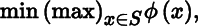
Static optimization theory is concerned with finding those points (if any) at which a real‐valued function ϕ, defined on a subset S of ℝn, has a minimum or a maximum. Two types of problems will be investigated in this chapter:
Unconstrained optimization (Sections 7.2–7.10) is concerned with the problem
where the point at which the extremum occurs is an interior point of S.
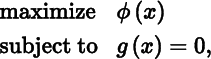
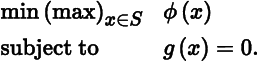
Optimization subject to constraints (Sections 7.11–7.16) is concerned with the problem of optimizing ϕ subject to m nonlinear equality constraints, say g1(x) = 0, …, gm(x) = 0. Letting g = (g1, g2, …, gm)′ and
the problem can be written as
or, equivalently, as
We shall not deal with inequality constraints.
2 UNCONSTRAINED OPTIMIZATION
In Sections 7.2–7.10, we wish to show how the one‐dimensional theory of maxima and minima of differentiable functions generalizes to functions of more than one variable. We start with some definitions.
Let ϕ : S → ℝ be a real‐valued function defined on a set S in ℝn, and let c be a point of S. We say that ϕ has a local minimum at c if there exists an n‐ball B(c) such that
ϕ has a strict local minimum at c if we can choose B(c) such that
ϕ has an absolute minimum at c if
ϕ has a strict absolute minimum at c if
The point c at which the minimum is attained is called a (strict) local minimum point for ϕ, or a (strict) absolute minimum point for ϕ on S, depending on the nature of the minimum.
If ϕ has a minimum at c, then the function −ϕ has a maximum at c. Each maximization problem can thus be converted to a minimization problem (and vice versa). For this reason, we lose no generality by treating minimization problems only.
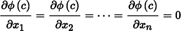
If c is an interior point of S, and ϕ is differentiable at c, then we say that c is a critical point (stationary point) of ϕ if
The function value ϕ(c) is then called the critical value of ϕ at c.
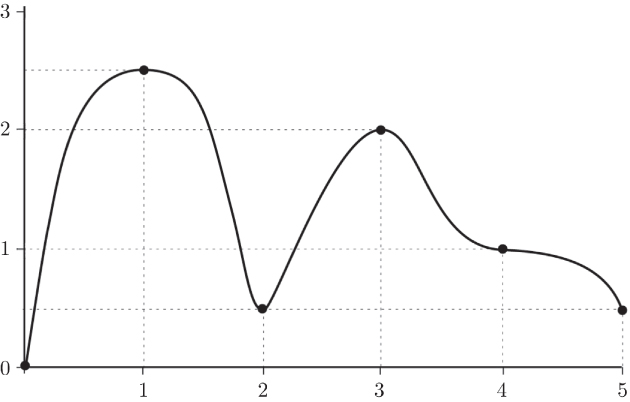
A critical point is called a saddle point if every n‐ball B(c) contains points x such that ϕ(x) > ϕ(c) and other points such that ϕ(x) < ϕ(c). In other words, a saddle point is a critical point which is neither a local minimum point nor a local maximum point. Figure 7.1 illustrates some of these concepts. The function ϕ is defined and continuous at [0, 5]. It has a strict absolute minimum at x = 0 and an absolute maximum (not strict if you look carefully) at x = 1. There are strict local minima at x = 2 and x = 5, and a strict local maximum at x = 3. At x = 4, the derivative ϕ′ is zero, but this is not an extremum point of ϕ; it is a saddle point.
Figure 7.1 Unconstrained optimization in one variable
3 THE EXISTENCE OF ABSOLUTE EXTREMA
In the example of Figure 7.1
, the function ϕ is continuous on the compact interval [0, 5] and has an absolute minimum (at x = 0) and an absolute maximum (at x = 1). That this is typical for continuous functions on compact sets is shown by the following fundamental result.
Exercises
1. The Weierstrass theorem is not, in general, correct if we drop any of the conditions, as the following three counterexamples demonstrate.
ϕ(x) = x, x ∈ (−1, 1), ϕ(−1) = ϕ(1) = 0,
ϕ(x) = x, x ∈ (−∞, ∞),
ϕ(x) = x/(1 − |x|), x ∈ (−1, 1).
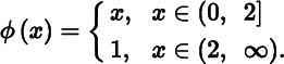
2. Consider the real‐valued function ϕ : (0, ∞) → ℝ defined by
The set (0, ∞) is neither bounded nor closed, and the function ϕ is not continuous on (0, ∞). Nevertheless, ϕ attains its maximum on (0, ∞). This shows that none of the conditions of the Weierstrass theorem are necessary.
4 NECESSARY CONDITIONS FOR A LOCAL MINIMUM
In the one‐dimensional case, if a real‐valued function ϕ, defined on an interval (a, b), has a local minimum at an interior point c of (a, b), and if ϕ has a derivative at c, then ϕ′(c) must be zero. This result, which relates zero derivatives and local extrema at interior points, can be generalized to the multivariable case as follows.
Exercises
1. Find the extreme value(s) of the following real‐valued functions defined on ℝ2 and determine whether they are minima or maxima:
ϕ(x, y) = x2 + xy + 2y2 + 3,
ϕ(x, y) = −x2 + xy − y2 + 2x + y,
ϕ(x, y) = (x − y + 1)2.
2. Answer the same questions as above for the following real‐valued functions defined for 0 ≤ x ≤ 2, 0 ≤ y ≤ 1:
ϕ(x, y) = x3 + 8y3 − 9xy + 1,
5 SUFFICIENT CONDITIONS FOR A LOCAL MINIMUM: FIRST‐DERIVATIVE TEST
In the one‐dimensional case, a sufficient condition for a differentiable function ϕ to have a minimum at an interior point c is that ϕ′(c) = 0 and that there exists an interval (a, b) containing c such that ϕ′(x) < 0 in (a, c) and ϕ′(x) > 0 in (c, b). (These conditions are not necessary, see Exercise 1 below.)
The multivariable generalization is as follows.
In this example, the function ϕ is strictly convex on ℝn, so that the condition of Theorem 7.3 is automatically fulfilled. We shall explore this in more detail in Section 7.7.
Exercises
1.
Consider the function ϕ(x) = x2[2 + sin(1/x)] when x ≠ 0 and ϕ(0) = 0. The function ϕ clearly has an absolute minimum at x = 0. Show that the derivative is ϕ′(x) = 4x + 2x sin(1/x) − cos(1/x) when x ≠ 0 and ϕ′(0) = 0. Show further that we can find values of x arbitrarily close to the origin such that xϕ′(x) < 0. Conclude that the converse of Theorem 7.3 is, in general, not true.
3.
Consider the function ϕ : ℝ2 → ℝ given by ϕ(x, y) = x2 + (1 + x)3y2. Prove that it has one local minimum (at the origin), no other critical points and no absolute minimum.
6 SUFFICIENT CONDITIONS FOR A LOCAL MINIMUM: SECOND‐DERIVATIVE TEST
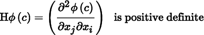
Another test for local extrema is based on the Hessian matrix.
In other words, Theorem 7.4 tells us that the conditions
and
(4)
together are sufficient for ϕ to have a strict local minimum at c. If we replace (4) by the condition that Hϕ(c) is negative definite, then we obtain sufficient conditions for a strict local maximum.
If the Hessian matrix Hϕ(c) is neither positive definite nor negative definite, but is nonsingular, then c cannot be a local extremum point (see Theorem 7.2); thus c is a saddle point.
In the case where Hϕ(c) is singular, we cannot tell whether c is a maximum point, a minimum point, or a saddle point (see Exercise 3 below). This shows that the converse of Theorem 7.4 is not true.
Exercises
1.
Show that the function ϕ : ℝ2 → ℝ defined by ϕ(x, y) = x4 + y4 − 2(x − y)2 has strict local minima at and , and a saddle point at (0, 0).
2.
Show that the function ϕ : ℝ2 → ℝ defined by ϕ(x, y) = (y − x2)(y − 2x2) has a local minimum along each straight line through the origin, but that ϕ has no local minimum at the origin. In fact, the origin is a saddle point.
3.
Consider the functions: (i) ϕ(x, y) = x4 + y4, (ii) ϕ(x, y) = −x4 − y4, and (iii) ϕ(x, y) = x3 + y3. For each of these functions show that the origin is a critical point and that the Hessian matrix is singular at the origin. Then prove that the origin is a minimum point, a maximum point, and a saddle point, respectively.
4.
Show that the function ϕ : ℝ3 → ℝ defined by ϕ(x, y, z) = xy + yz + zx has a saddle point at the origin, and no other critical points.
5.
Consider the function ϕ : ℝ2 → ℝ defined by ϕ(x, y) = x3 − 3xy2 + y4. Find the critical points of ϕ and show that ϕ has two strict local minima and one saddle point.
7 CHARACTERIZATION OF DIFFERENTIABLE CONVEX FUNCTIONS
So far, we have dealt only with local extrema. However, in the optimization problems that arise in economics (among other disciplines) we are usually interested in finding absolute extrema. The importance of convex (and concave) functions in optimization comes from the fact that every local minimum (maximum) of such a function is an absolute minimum (maximum). Before we prove this statement (Theorem 7.8), let us study convex (concave) functions in some more detail.
Recall that a set S in ℝn is convex if for all x, y in S and all λ ∈ (0, 1),
and a real‐valued function ϕ, defined on a convex set S in ℝn, is convex if for all x, y ∈ S and all λ ∈ (0, 1),
(5)
If (5) is satisfied with strict inequality for x ≠ y, then we call ϕ strictly convex. If ϕ is (strictly) convex, then −ϕ is (strictly) concave.
In this section, we consider (strictly) convex functions that are differentiable, but not necessarily twice differentiable. In the next section, we consider twice differentiable convex functions.
We first show that ϕ is convex if and only if at any point the tangent hyperplane is below the graph of ϕ (or coincides with it).
Another characterization of differentiable functions exploits the fact that, in the one‐dimensional case, the first derivative of a convex function is monotonically nondecreasing. The generalization of this property to the multivariable case is contained in Theorem 7.6.
Exercises
1.
Show that the function ϕ(x, y) = x + y(y − 1) is convex. Is ϕ strictly convex?
2.
Prove that ϕ(x) = x4 is strictly convex.
8 CHARACTERIZATION OF TWICE DIFFERENTIABLE CONVEX FUNCTIONS
Both characterizations of differentiable convex functions (Theorems 7.5 and 7.6
) involved conditions on two points. For twice differentiable functions, there is a characterization that involves only one point.
Exercises
1.
Repeat Exercise 1 in Section 4.9 using Theorem 7.7.
2.
Show that the function ϕ(x) = xp, p > 1 is strictly convex on [0, ∞).
3.
Show that the function ϕ(x) = x′x, defined on ℝn, is strictly convex.
4. Consider the CES (constant elasticity of substitution) production function
defined for x > 0 and y > 0. Show that ϕ is convex if ρ ≤ −1, and concave if ρ ≥ −1 (and ρ ≠ 0). What happens if ρ = −1?
9 SUFFICIENT CONDITIONS FOR AN ABSOLUTE MINIMUM
The convexity (concavity) of a function enables us to find the absolute minimum (maximum) of the function, since every local minimum (maximum) of such a function is an absolute minimum (maximum).
To check whether a given differentiable function is (strictly) convex, we thus have four criteria at our disposal: the definition in Section 4.9, Theorems 7.5 and 7.6
, and, if the function is twice differentiable, Theorem 7.7.
Exercises
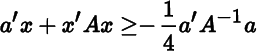
1. Let a be an n × 1 vector and A a positive definite n × n matrix. Show that
for every x in ℝn. For which value of x does the function ϕ(x) = a′x + x′Ax attain its minimum value?
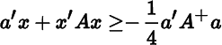
2. (More difficult.) If A is positive semidefinite and AA+a = a, show that
for every x in ℝn? What happens when AA+a ≠ a?
10 MONOTONIC TRANSFORMATIONS
To complete our discussion of unconstrained optimization, we shall prove the useful, if simple, fact that minimizing a function is equivalent to minimizing a monotonically increasing transformation of that function.
Exercise
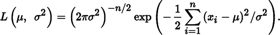
1. Consider the likelihood function
Use Theorem 7.9 to maximize L with respect to μ and σ2.
11 OPTIMIZATION SUBJECT TO CONSTRAINTS
Let ϕ : S → ℝ be a real‐valued function defined on a set S in ℝn. Hitherto we have considered optimization problems of the type
It may happen, however, that the variables x1, …, xn are subject to certain constraints, say g1(x) = 0, …, gm(x) = 0. Our problem is now
where g : S → ℝm is the vector function g = (g1, g2, …, gm)′. This is known as a constrained minimization problem (or a minimization problem subject to equality constraints), and the most convenient way of solving it is, in general, to use the Lagrange multiplier theory. In the remainder of this chapter, we shall study this important theory in some detail.
We start our discussion with some definitions. The subset of S on which g vanishes, that is,
is known as the opportunity set (constraint set). Let c be a point of Γ. We say that ϕ has a local minimum at c under the constraint g(x) = 0 if there exists an n‐ball B(c) such that
ϕ has a strict local minimum at c under the constraint g(x) = 0 if we can choose B(c) such that
ϕ has an absolute minimum at c under the constraint g(x) = 0 if
and ϕ has a strict absolute minimum at c under the constraint g(x) = 0 if
12 NECESSARY CONDITIONS FOR A LOCAL MINIMUM UNDER CONSTRAINTS
The next theorem gives a necessary condition for a constrained minimum to occur at a given point.
Exercises
1. Consider the problem
By using Lagrange's method, show that the minimum point is (0,0) with λ = 1. Next, consider the Lagrangian function
and show that ψ has a saddle point at (0,0). That is, the point (0,0) does not minimize ψ. (This shows that it is not correct to say that minimizing a function subject to constraints is equivalent to minimizing the Lagrangian function.)
2. Solve the following problems by using the Lagrange multiplier method:
for all positive real numbers x1, …, xn. (Compare Section 11.4.)
4. Solve the problem
5. Solve the following utility maximization problem:
with respect to x1 and x2 (x1 > 0, x2 > 0).
13 SUFFICIENT CONDITIONS FOR A LOCAL MINIMUM UNDER CONSTRAINTS
In the previous section, we obtained conditions that are necessary for a function to achieve a local minimum or maximum subject to equality constraints. To investigate whether a given critical point actually yields a minimum, maximum, or neither, it is often practical to proceed on an ad hoc basis. If this fails, the following theorem provides sufficient conditions to ensure the existence of a constrained minimum or maximum at a critical point.
The difficulty in applying Theorem 7.11 lies, of course, in the verification of the second‐order condition. This condition requires that
where
Several sets of necessary and sufficient conditions exist for a quadratic form to be positive definite under linear constraints, and one of these is discussed in Section 3.11. The following theorem is therefore easily proved.
Exercises
1.
Discuss the second‐order conditions for the constrained optimization problems in Exercise 2 in Section 7.12.
2.
Answer the same question as above for Exercises 4 and 5 in Section 7.12.
3.
Compare Example 7.4 and the solution method of Section 7.13 with Example 7.3 and the solution method of Section 7.12.
14 SUFFICIENT CONDITIONS FOR AN ABSOLUTE MINIMUM UNDER CONSTRAINTS
The Lagrange theorem (Theorem 7.10) gives necessary conditions for a local (and hence also for an absolute) constrained extremum to occur at a given point. In Theorem 7.11, we obtained sufficient conditions for a local constrained extremum. To find sufficient conditions for an absolute constrained extremum, we proceed as in the unconstrained case (Section 7.9) and impose appropriate convexity (concavity) conditions.
To prove that the Lagrangian function ψ is (strictly) convex or (strictly) concave, we can use the definition in Section 4.9, Theorem 7.5 or Theorem 7.6, or (if ψ is twice differentiable) Theorem 7.7. In addition, we observe that
if the constraints g1(x), …, gm(x) are all linear and ϕ(x) is (strictly) convex, then ψ(x) is (strictly) convex.
In fact, (a) is a special case of
if the functions λ1g1(x), …, λmgm(x) are all concave (that is, for i = 1, 2, …, m, either gi(x) is concave and λi ≥ 0, or gi(x) is convex and λi ≤ 0) and if ϕ(x) is convex, then ψ(x) is convex; furthermore, if at least one of these m + 1 conditions is strict, then ψ(x) is strictly convex.
15 A NOTE ON CONSTRAINTS IN MATRIX FORM
Let ϕ : S → ℝ be a real‐valued function defined on a set S in ℝn × q, and let G : S → ℝm × p be a matrix function defined on S. We shall frequently encounter the problem
This problem is, of course, mathematically equivalent to the case where X and G are vectors rather than matrices, so all theorems remain valid. We now introduce mp multipliers λij (one for each constraint gij(X) = 0, i = 1, …, m; j = 1, …, p), and define the m × p matrix of Lagrange multipliers L = (λij). The Lagrangian function then takes the convenient form
16 ECONOMIC INTERPRETATION OF LAGRANGE MULTIPLIERS
Consider the constrained minimization problem
where ϕ is a real‐valued function defined on an open set S in ℝn, g is a vector function defined on S with values in ℝm(m < n) and b = (b1, …, bm)′ is a given m × 1 vector of constants (parameters). In this section, we shall examine how the optimal solution of this constrained minimization problem changes when the parameters change.
We shall assume that
ϕ and g are twice continuously differentiable on S,
(first‐order conditions) there exist points x0 = (x01, …, x0n)′ in S and l0 = (λ01, …, λ0m)′ in ℝm such that
(38)
(39)
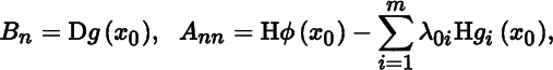
Now let
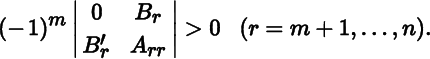
and define, for r = 1, 2, …, n, Br as the m × r matrix whose columns are the first r columns of Bn, and Arr as the r × r matrix in the top left corner of Ann. In addition to (i) and (ii), we assume that
|Bm| ≠ 0,
(second‐order conditions)
These assumptions are sufficient (in fact, more than sufficient) for the function ϕ to have a strict local minimum at x0 under the constraint g(x) = b (see Theorem 7.12).
The vectors x0 and l0 for which the first‐order conditions (38) and (39) are satisfied will, in general, depend on the parameter vector b. The question is whether x0 and l0 are differentiable functions of b. Given assumptions (i)–(iv), this question can be answered in the affirmative. By using the implicit function theorem (Theorem 7.15), we can show that there exists an m‐ball B(0) with the origin as its center, and unique functions x* and l* defined on B(0) with values in ℝn and ℝm, respectively, such that
x*(0) = x0, l*(0) = l0,
Dϕ(x* (y)) = (l*(y))′Dg(x*(y)) for all y in B(0),
g(x*(y)) = b for all y in B(0),
the functions x* and l* are continuously differentiable on B(0).
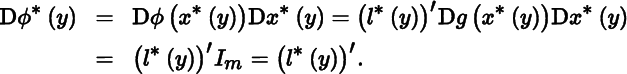
Now consider the real‐valued function ϕ* defined on B(0) by the equation
We first differentiate both sides of (c). This gives
(40)
using the chain rule. Next we differentiate ϕ*. Using (again) the chain rule, (b) and (40), we obtain
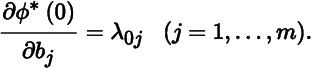
In particular, at y = 0,
Thus, the Lagrange multiplier λ0j measures the rate at which the optimal value of the objective function changes with respect to a small change in the right‐hand side of the jth constraint. For example, suppose we are maximizing a firm's profit subject to one resource limitation, then the Lagrange multiplier λ0 is the extra profit that could be earned if the firm had one more unit of the resource, and therefore represents the maximum price the firm is willing to pay for this additional unit. For this reason, λ0 is often referred to as a shadow price.
Exercise
1.
In Exercise 2 in Section 7.12, find whether a small relaxation of the constraint will increase or decrease the optimal function value. At what rate?
APPENDIX: THE IMPLICIT FUNCTION THEOREM
Let f : ℝm + k → ℝm be a linear function defined by
where, as the notation indicates, points in ℝm + k are denoted by (x; t) with x ∈ ℝm and t ∈ ℝk. If the m × m matrix A is nonsingular, then there exists a unique function g : ℝk → ℝm such that
g(0) = 0,
f(g(t); t) = 0 for all t ∈ ℝk,
g is infinitely times differentiable on ℝk.
This unique function is, of course,
The implicit function theorem asserts that a similar conclusion holds for certain differentiable transformations which are not linear. In this Appendix, we present (without proof) three versions of the implicit function theorem, each one being useful in slightly different circumstances.
BIBLIOGRAPHICAL NOTES
1. Apostol (1974, Chapter 13) has a good discussion of implicit functions and extremum problems. See also Luenberger (1969) and Sydsæter (1981, Chapter 5).
9 and §14. For an interesting approach to absolute minima with applications in statistics, see Rolle (1996).
Appendix. There are many versions of the implicit function theorem, but Theorem 7.15 is what most authors would call ‘the’ implicit function theorem. See Dieudonné (1969, Theorem 10.2.1) or Apostol (1974, Theorem 13.7). Theorems 7.14 and 7.16 are less often presented. See, however, Young (1910, Section 38).
 or, equivalently, as
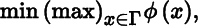

 and
and  , and a saddle point at (0, 0).