
Chapter 9
Demystifying Sampling Distributions and the Central Limit Theorem
IN THIS CHAPTER
![]() Identifying a sampling distribution
Identifying a sampling distribution
![]() Interpreting the central limit theorem
Interpreting the central limit theorem
![]() Using the central limit theorem to find probabilities
Using the central limit theorem to find probabilities
![]() Knowing when you can use the central limit theorem and when you can’t
Knowing when you can use the central limit theorem and when you can’t
Many instructors love to talk on and on about the glories of the central limit theorem (CLT) and how important sampling distributions are to their being, but instructors should all face the fact that you probably don’t care about these ideas that much. You just want to get through your class, right? And of course, sampling distributions and any topics related to a “theorem” aren’t the easiest subjects on the statistics syllabus (most statistics teaching circles consider them to be the hardest and the most important — what luck). Before you decide to pack it in and call it quits, know that I feel your pain, and I’m here to help.
In this chapter, more than in any other, I think of you as being on a “need-to-know-only” basis. No extra stuff, no frilly theoretical gibberish, no talking about the CLT like it’s the best thing since sliced bread, no pining of how “beautiful” all these ideas are. I give you the information that you need to know, when you need to know it, and with plenty of problems to practice. I don’t pull any punches here — this stuff is complicated — but I try to break it down so you can focus on only the items you’re most likely to face, without the big sales pitch. Can you do it? Yes, you can. Time to get started.
Exactly What Is a Sampling Distribution?
A sampling distribution is basically a histogram of all the values that a sample statistic can take on. Sampling distributions are important because when you take a sample from a population, you base all your conclusions on that one sample, and sample results vary. To know how precise your particular sample mean is, you have to think about all the possible sample means you’d get if you took all possible samples of the same size from the population. In other words, to interpret your sample results, you have to know where they stand among the crowd. The crowd of all possible sample statistics you can possibly get is the sampling distribution.
If your data is numerical and your sample statistic is a mean of a sample of size n, you should compare that data to all possible sample means of size n from that population. You take the sampling distribution for the sample mean, also known as the sampling distribution for ![]() . A sampling distribution, like any other distribution, has a shape, a center, and a measure of variability. Here are some properties of the sampling distribution for
. A sampling distribution, like any other distribution, has a shape, a center, and a measure of variability. Here are some properties of the sampling distribution for ![]() :
:
- If the population already has a normal distribution, the sampling distribution of
 also has a normal distribution.
 -
 has an approximate normal distribution if the sample size (n) is large enough — regardless of what the histogram of the population looks like (due to the central limit theorem [CLT] — the part that instructors get all excited and starry-eyed talking about; see the following section).
How large is “large enough” to make your calculations work? Statisticians bounce the number
 around a lot. The bigger, the better, of course, but the sample size should be at least 30. That means you can take your mean, convert it to a standard (Z-) score, and use the Z-table to find probabilities for it. (See Chapter 6 for more on standard scores.) All you need to know is what mean and standard deviation to use.
 - The mean of all the possible values of
 is equal to the mean of the population, μ.
 -
You measure the variability of
 by the standard error. The standard error of a statistic (like the mean) is the standard deviation of all the possible values of the statistic. In other words, the standard error of
  is the standard deviation of all possible sample means of size n you take from the population.
Here’s a nice formula for standard error: The standard error of
 is equal to the standard deviation of the population divided by the square root of n. The notation for this is
 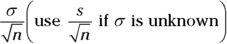 .
.As the sample size gets larger, the standard error goes down. A smaller standard error is good because it says that the sample means don’t vary by much when the sample sizes get large (your sample mean is precise, as long as your n is large and your data was collected properly).
If your sample statistic is a proportion from a sample of size n, you should compare it to all possible sample proportions from samples of size n from that population. In other words, you find the sampling distribution for the sample proportion, or the sampling distribution for ![]() . Here are some properties of the sampling distribution for
. Here are some properties of the sampling distribution for ![]() :
:
-
The sampling distribution has an approximate normal distribution as long as the sample size is “large enough.” (This is due to the CLT; see the following section.)
How large is “large enough” to make the distribution work? Where p is the proportion of the population that have the characteristic of interest,
 must be at least 10 and
  must be at least 10.
 - The mean of all the values of
 is equal to the original population proportion p.
 - The standard error of
 is equal to
  , where p is the population proportion. Notice again the formula has a square root of n in the denominator, similar to the standard error of
  .
. - As the sample size gets larger, the standard error of
 goes down.
See the following for an example of depicting the sampling distribution for the sample mean.
 Q. Suppose that you take a sample of 100 from a population that has a normal distribution with mean 50 and standard deviation 15.
- What sample size condition do you need to check here (if any)?
- Where’s the center of the sampling distribution for
 ?
? - What’s the standard error?
A. Remember to check the original distribution to see whether it’s normal before talking about the sampling distribution of the mean.
- This sample distribution already has a normal distribution, so you don’t need approximations. The distribution of
 has an exact normal distribution for any sample size. (Don’t get so caught up in the
  condition that you forget situations where the data has a normal distribution to begin with. In these cases, you don’t need to meet any sample size conditions; they hold true for any n.)
 - The center is equal to the mean of the population, which is 50 in this case.
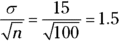
- The standard error is the standard deviation of the population (15) divided by the square root of the sample size (100); in this case, 1.5.
1 Suppose that you take a sample of 100 from a skewed population with mean 50 and standard deviation 15.
- What sample size condition do you need to check here (if any)?
- What’s the shape and center of the sampling distribution for
 ?
? - What’s the standard error?
2 Suppose that you take a sample of 100 from a population that contains 45 percent Democrats.
- What sample size condition do you need to check here (if any)?
- What’s the standard error of
 ?
? - Compare the standard errors of
 for
for  ,
,  , and
, and  and comment.
Clearing Up the Central Limit Theorem (Once and for All)
The reason that the sampling distributions for ![]() and
and ![]() turn out to be normal for large enough samples is because when you’re taking averages, everything averages out to the middle. Even if you roll a die with an equal chance of getting a 1, 2, 3, 4, 5, or 6, if you roll it enough times, all the 6s you get average out with all the 1s you get, and that average is 3.5. All the 5s you get average out with all the 2s you get, and that average is 3.5. All the 4s you get average out with all the 3s you get, and that average is (you guessed it) 3.5. Where does the 3.5 come from? From the average of the original population of values 1, 2, 3, 4, 5, 6. And the more times you roll the die, the harder and harder it is to get an average that moves far from 3.5, because averages based on large sample sizes don’t change much.
turn out to be normal for large enough samples is because when you’re taking averages, everything averages out to the middle. Even if you roll a die with an equal chance of getting a 1, 2, 3, 4, 5, or 6, if you roll it enough times, all the 6s you get average out with all the 1s you get, and that average is 3.5. All the 5s you get average out with all the 2s you get, and that average is 3.5. All the 4s you get average out with all the 3s you get, and that average is (you guessed it) 3.5. Where does the 3.5 come from? From the average of the original population of values 1, 2, 3, 4, 5, 6. And the more times you roll the die, the harder and harder it is to get an average that moves far from 3.5, because averages based on large sample sizes don’t change much.
What that means for you is, when you estimate the population mean by using a sample mean (Chapter 11), or when you test a claim about the population mean by using a sample mean (Chapter 13), you can forecast the precision of your results because of the standard error. And what do you need to know to get the standard error of ![]() ? Two things:
? Two things:
- The standard deviation of the population (estimate it with sample standard deviation, s, if you don’t have it; see Chapter 4)
- The sample size
And you can easily get both numbers from your one single sample. So wow, you can compare your one sample mean to all the other sample means out there, without having to look at any of the others. As Linus would say, “That’s what the central limit theorem is all about, Charlie Brown.”
 Here’s a condensed version of the central limit theorem (CLT) for means that likely resembles any used by instructors. For any population with mean
 ![]() and standard deviation
and standard deviation ![]() :
:
- The distribution of all possible sample means,
 , is approximately normal. (See Chapter 6 for more about normal distribution.)
 - The larger the sample size (n), the better the normal approximation (most statisticians agree that an n of at least 30 does a reasonable job in most cases).
- The mean of the distribution of sample means is also
 .
. - The standard error of the sample means is
 . It decreases as n increases.
 - If the original data has a normal distribution, the approximation is exact, no matter what the sample size is.
Here’s a condensed version of the theorem applied to proportions. For any population of data with p as the overall population percentage:
- The distribution of all possible sample proportions
 is approximately normal, provided that the sample size is large enough. That is, both
  and
and  must be at least 10. (See Chapter 6 for the normal distribution.)
 - The larger the sample size (n), the better the normal approximation.
- The mean of the distribution of sample proportions is also p.
- The standard error of the sample proportions is
 . It decreases as n increases.
See the following for an example of using the CLT with sample proportions.
Q. Suppose that you want to find p where p = the proportion of college students in the United States who make more than a million dollars a year. Obviously, p is very small (most likely around ![]() ), meaning the data is very skewed.
), meaning the data is very skewed.
- How big of a sample size do you need to take to use the CLT to talk about your results?
- Suppose that you live in a dream world where p equals 0.5. Now what sample size do you need to meet the conditions for the CLT?
- Explain why you think that skewed data may require a larger sample size than a symmetric data set for the CLT to kick in.
A. Check to be sure the “is it large enough” condition is met before applying the CLT.
- You need
 to be at least 10; so,
  , which says
  . And checking
  gives you
 , which is
  , which is fine. But wow, the skewness creates a great need for size. You need a larger sample size to meet the conditions with skewed data (since p is far from
  , the case where the distribution is symmetric).
 - You need
 to be at least 10; so,
  , which says
  . And checking
  gives you
  also, so both conditions check out if n is at least 20. You don’t need a very large sample size to meet the conditions with symmetric data
  .
. - With a symmetric data set, the data averages out to the mean fairly quickly because the data is balanced on each side of the mean. Skewed data takes longer to average out to the middle, because when sample sizes are small, you’re more likely to choose values that fall in the big lump of data, not in the tails.
3 How do you recognize that a statistical problem requires you to use the CLT? Think of one or two clues you can look for. (Assume quantitative data.)
4 Suppose that a coin is fair (so ![]() for heads or tails).
for heads or tails).
- Guess how many times you have to flip the coin to get the standard error down to only 1 percent (don’t do any calculations).
- Now use the standard error formula to figure it out.
Finding Probabilities with the Central Limit Theorem
You use ![]() to estimate or test the population mean (in the case of numerical data), and you use
to estimate or test the population mean (in the case of numerical data), and you use ![]() to estimate or test the population proportion (in the case of categorical data). Because the sampling distributions of
to estimate or test the population proportion (in the case of categorical data). Because the sampling distributions of ![]() and
and ![]() are both approximately normal for large enough sample sizes, you’re back into familiar territory somewhat. If you want to find the probability for
are both approximately normal for large enough sample sizes, you’re back into familiar territory somewhat. If you want to find the probability for ![]() where
where ![]() has a normal distribution, all you have to do is convert it to a standard score, look up the value on the Z-table (see the Appendix), and take it from there (and check out Chapter 6 for more on normal distribution).
has a normal distribution, all you have to do is convert it to a standard score, look up the value on the Z-table (see the Appendix), and take it from there (and check out Chapter 6 for more on normal distribution).
The only question is how to convert to a standard score. To convert to a standard score, you first find the mean and standard deviation. After you find these figures, you take the number that you want to convert, subtract the mean, and then divide the result by the standard deviation (see Chapter 6 for details). In this chapter, you do everything like you do in Chapter 6, except you replace the standard deviation with the standard error. So in the case of the sample mean, you don’t divide by ![]() ; you divide by
; you divide by ![]() . Then you look it up on the Z-table and finish the problem from there as usual.
. Then you look it up on the Z-table and finish the problem from there as usual.
See the following for an example of finding a probability for the sample mean.
Q. Suppose that you have a population with mean 50 and standard deviation 10. Select a random sample of 40. What’s the chance that the mean will be less than 55?
A. To find this probability, you take the sample mean, 55, and convert it to a standard score, using  . This gives you
  . Using the Z-table, the probability of being less than 3.16 is 0.9993. So the probability that the sample mean is less than 55 is equal to the probability that Z is less than 3.16, which is 0.9992, or 99.92 percent.
5 Suppose that you have a normal population of quiz scores with mean 40 and standard deviation 10.
- Select a random sample of 40. What’s the chance that the mean of the quiz scores won’t exceed 45?
- Select one individual from the population. What’s the chance that his/her quiz score won’t exceed 45?
6 You assume that the annual incomes for certain workers are normal with a mean of $28,500 and a standard deviation of $2,400.
- What’s the chance that a randomly selected employee makes more than $30,000?
- What’s the chance that 36 randomly selected employees make more than $30,000, on average?
7 Suppose that studies claim that 40 percent of cellphone owners use their phones in the car while driving. What’s the chance that more than 425 out of a random sample of 1,000 cellphone owners say they use their phones while driving?
8 What’s the chance that a fair coin comes up heads more than 60 times when you toss it 100 times?
When Your Sample’s Too Small: Employing the t-Distribution
In a case where the sample size is small (and by small, I mean dropping below 30 or so), you have less information on which to base your conclusions about the mean. Another drawback is that you can’t rely on the standard normal distribution to compare your results, because the central limit theorem (CLT) can’t kick in yet. So what do you do in situations where the sample size isn’t big enough to use the standard normal distribution? You use a different distribution — the t-distribution (see Chapter 8).
You use the t-distribution more when dealing with confidence intervals (see Chapter 11) and hypothesis tests (see Chapter 13). In this chapter, you practice understanding and using the t-table (see the Appendix).
See the following for an example of a problem involving averages that use the t-distribution.
Q. Suppose that you find the mean of 10 quiz scores, convert it to a standard score, and check the table to find out it’s equal to the 99th percentile.
- What’s the standard score?
- Compare the result to the standard score you have to get to be at the 99th percentile on the Z-distribution.
A. t-distributions push you farther out to get to the same percentile a Z-distribution would.
- Your sample size is
 , so you need the t-distribution with
  degrees of freedom, also known as the
  distribution. Using the t-table, the value at the 99th percentile is 2.821. (Remember to go to Row 9 of the t-table and find the number that falls in the .01 column, since .99 is the probability of being less than the value, and .01 is the greater-than probability — shown in table.)
 - Using the Z-distribution (also in the Appendix), the standard score associated with the 99th percentile is 2.33, which is much smaller than the 2.821 from part a of this question. The number is smaller because the t-distribution is flatter than the Z, with more area or probability out in the tails. So to get all the way out to the 99th percentile, you have to go farther out on the t-distribution than on the Z.
9 Suppose that the average length of stay in Europe for American tourists is 17 days, with standard deviation 4.5. You choose a random sample of 16 American tourists. The sample of 16 stay an average of 18.5 days or more. What’s the chance of that happening?
10 Suppose that a class’s test scores have a mean of 80 and standard deviation of 5. You choose 25 students from the class. What’s the chance that the group’s average test score is more than 82?
11 Suppose that you want to sample expensive computer chips, but you can have only ![]() of them. Should you continue the experiment?
of them. Should you continue the experiment?
12 Suppose that you collect data on 10 products and check their weights. The average should be 10 ounces, but your sample mean is 9 ounces with standard deviation 2 ounces.
- Find the standard score.
- What percentile is the standard score found in part a of this question closest to?
- Suppose that the mean really is 10 ounces. Do you find these results unusual? Use probabilities to explain.
Answers to Problems in Sampling Distributions and the Central Limit Theorem
1 The fact that you have a skewed population to start with and that you end up using a normal distribution in the end are important parts of the central limit theorem (CLT).
- The condition is
 , which you meet.
 - The shape is approximately normal by the CLT. The center is the population mean, 50.
- The standard error is
 . Notice that when the problem gives you the population standard deviation
  , you use it in the formula for standard error. If not, you use the sample standard deviation.
 Checking conditions is becoming more and more of an “in” thing in statistics classes, so be sure you put it on your radar screen. Check conditions before you proceed.
2 Here’s a situation where you deal with percents and want a probability. The CLT is your route, provided your conditions check out.
- You need to check
 and
and 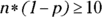 . In this case, you have
  , which is fine, and
  , which is also fine.
 - The standard error is
 .
. - The standard errors for
 respectively, are: 0.050,
  The standard errors get smaller as n increases, meaning you get more and more precise with your sample proportions as the sample size goes up.
3 The main clue is when you have to find a probability about an average with the data not normal, or a proportion.
Watch for little words or phrases that can really help you lock on to a problem and know how to work it. I know this sounds cheesy, but there’s no better (statistical) feeling than the feeling that comes over you when you recognize how to do a problem. Practicing that skill while the points are free is always better than sweating over the skill when the points cost you something (like on an exam).
4 I’m guessing that you guessed too high in your answer to part a of this question.
- Whatever you guessed is fine; after all, it’s just a guess.
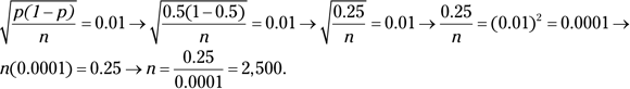
- The actual answer is 2,500. You can use trial and error and plug different values for n into the standard error formula to see which n gets you a standard error of 1 percent (or 0.01). Or if you don’t have that kind of time, you can take the standard error formula, plug in the parts you know, and use algebra to solve for n. Here’s how:
I know what you’re thinking: Will my instructor really ask a question like Question 4b? Probably not. But if you train at a little higher setting of the bar, you’re more likely to jump over the real setting of the bar in a test situation. If you solved Question 4, great. If not, no big deal.
5 Problems such as this require quite a bit of calculation compared to other types of statistical problems. Hang in there; show all your steps, and you can make it.
For this problem and the remaining problems in this chapter, I write down every step using probability notation to keep all the information organized and to show you the kind of work your instructor will likely want to see from you when you do these problems. I first write down what I want, in terms of a probability, and then I use the appropriate Z-formula to change the given number to a standard score, and then I look it up on the Z- (or t-) table. Finally, I take 1 minus that value if I’m looking for the probability of being greater than (rather than less than), for example.
-
Not exceeding 45 means < 45, so you want
 or 99.92%
by looking it up on the Z-table (see the Appendix).
- In this case, you focus on one individual, not the average, so you don’t use sampling distributions to answer it; you use the old Z-formula (see Chapter 6). That means you want
 . Take 45 and convert it to a Z-score (subtract the mean, 40, and divide by the standard deviation, 10) to get
  . The probability of being less than 0.5 using the Z-table is 0.6915, or 69.15%.
Be on the lookout for two-part problems where, in one part, you find a probability about a sample mean, and in the other part, you find the probability about a single individual. Both convert to a Z-score and use the Z-table in the Appendix, but the difference is the first part requires you to divide by the standard error, and the second part requires you to divide by the standard deviation. Instructors really want you to understand these ideas, and they put them on exams almost without exception.
6 Here’s another problem that dedicates one part to a probability about one individual (part a) and another part to a sample of individuals (part b).
- You have
 . You get this answer by changing 30,000 to a Z-score of 0.63, looking up 0.63 on the Z-table, and taking 1 minus the result because you have a greater-than probability.
 - Here, you want

The Z-value of 3.75 is pretty much off the chart when you look at the Z-table. If this happens to you, use the last value on the chart (in this case, 3.69) and say that the probability of being beyond 3.75 on the Z-table has to be smaller than the probability of being beyond 3.69, the last value on the chart. The percentile for 3.69 is 99.99 percent, so the area beyond (above) that is
 (or 0.0001). Therefore, you can say that the probability of 36 workers making more than $30,000 is less than 0.0001.
7 Here you have to find the sample proportion by using the information in the problem. Because 425 people out of the sample of 1,000 say they use cellphones while driving, you take 425 divided by 1,000 to get your sample proportion, which is 0.425. Now you want to know how likely it is to get results like that (or greater than that). That means you want

or 4.75%.
If you’re given the sample size and the number of individuals in the group you’re interested in, divide those to get your sample proportion.
8 A fair coin means ![]() , where p is the proportion of heads or tails in the population of all possible tosses. In this case, you want the probability that your sample proportion is beyond
, where p is the proportion of heads or tails in the population of all possible tosses. In this case, you want the probability that your sample proportion is beyond ![]() . So you have
. So you have  or 2.07%.
9 You have 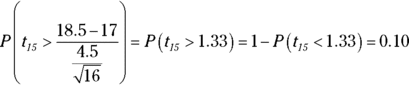 or 10%.
First, change 18.5 to a value on the t-distribution (1.33). Then look at the t-table (Appendix) in the row for ![]() degrees of freedom, and find the number closest to 1.33 (which is 1.341). This gives you the answer 0.10.
degrees of freedom, and find the number closest to 1.33 (which is 1.341). This gives you the answer 0.10.
10 You want 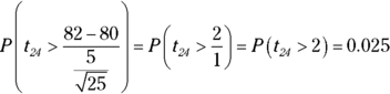 or 2.5%.
First, change the 82 to a value on the t-distribution (2), and then look at the t-table in the row for ![]() degrees of freedom, and find the number closest to 2 (which is 2.064). This gives you the answer 0.025.
degrees of freedom, and find the number closest to 2 (which is 2.064). This gives you the answer 0.025.
11 The experiment might not be worth it because the values are so large on the t-distribution with two degrees of freedom; you have to deal with too much variability in what you expect to find.
12 Here you compare what you expect to see with what you actually get (which comes up in hypothesis testing; see Chapter 13). The basic information here is that you have ![]()
-
The standard score is

Note: This number is negative, meaning you’re 1.58 standard deviations below the mean on the
 distribution
  . There are no negative values on the t-table. What you need to do is take 100 percent minus the percentile you get for the positive value 1.58. Now 1.58 lies between the 90th and 95th percentiles on the
  distribution, so
  lies between the
  percentile and the
  percentile on the
  distribution. To get percentiles for negative standard scores on the t-table, take 100 percent minus the percentile for the positive version of the standard score. Because the t-distribution is symmetric, the area below the negative standard score is equal to the area above the positive version of the standard score. And the area above the positive standard score is 100 percent minus what’s found on the t-table.
 - Your standard score of 1.58 from part a of this question is between the 90th and 95th percentiles on the
 distribution (that is, between 1.383 and 1.833) — a little closer to the 90th. That’s the best answer you can give using the t-table.
 - The results aren’t entirely unusual because, according to part b of this question, they happen between 5 and 10 percent of the time.