
Chapter 13
Testing Hypotheses
IN THIS CHAPTER
![]() Understanding the basic parts of a hypothesis test
Understanding the basic parts of a hypothesis test
![]() Setting up your null and alternative hypotheses
Setting up your null and alternative hypotheses
![]() Calculating test statistics
Calculating test statistics
![]() Determining the critical values
Determining the critical values
![]() Drawing conclusions and making interpretations
Drawing conclusions and making interpretations
A hypothesis test is a statistical procedure designed to test a claim about a population. In other words, someone proposes a certain parameter, and you want to test the claim by using data. Testing a hypothesis is different from a confidence interval situation, where you have no idea what the parameter is and you use your data to estimate it.
In this chapter, you review the basic ideas and steps of conducting a hypothesis test, and you practice setting up and carrying out the most common hypothesis tests: the tests for a population mean, a population proportion, two population means, and two population proportions. You also practice working with the t-distribution, which you use in situations where the sample sizes are too small to use the Z-distribution, or if the population standard deviation, ![]() , is unknown (see Chapters 7 and 8 for more on the Z- and t-distributions).
, is unknown (see Chapters 7 and 8 for more on the Z- and t-distributions).
The most common hypothesis test is the test for one population mean. Someone is claiming that the population mean is one value, and you are testing that claim because you believe it to be false. In this first section, you go through each step of a hypothesis test using the situation where you are testing one population mean. You also assume that the population standard deviation, ![]() , is known and that you have either a normal distribution for your population or a large enough sample size (sample
, is known and that you have either a normal distribution for your population or a large enough sample size (sample ![]() ).
).
Walking Through a Hypothesis Test
Every hypothesis test contains two hypotheses. The first hypothesis is called the null hypothesis, denoted Ho (pronounced “H naught”). The null hypothesis states that the population parameter is equal to the claimed value. For example, if you claim that the average test score for a population of students is 75, you have Ho: ![]() . In general, when you are conducting a hypothesis test about the population mean, you use
. In general, when you are conducting a hypothesis test about the population mean, you use ![]() to denote the claimed value of
to denote the claimed value of ![]() in the null hypothesis (for example, 75).
in the null hypothesis (for example, 75).
Along with every null hypothesis is an alternative hypothesis, denoted Ha (or ![]() ). If Ho turns out to be false, you conclude that the alternative hypothesis is true. Three possibilities exist for the second or alternative hypothesis, denoted Ha:
). If Ho turns out to be false, you conclude that the alternative hypothesis is true. Three possibilities exist for the second or alternative hypothesis, denoted Ha:
- The population parameter is not equal to the claimed value, written as Ha:
 .
. - The population parameter is greater than the claimed value, denoted Ha:
 .
. - The population parameter is less than the claimed value, denoted Ha:
 .
.
Which alternative hypothesis you choose when setting up your hypothesis test depends on what you want to conclude, should you have enough evidence to refute the claim (Ho). If someone claims that the average test score is higher than 75, you have Ha: ![]() . If someone thinks that the percentage of students who own cellphones is less than 65 percent, you have Ha:
. If someone thinks that the percentage of students who own cellphones is less than 65 percent, you have Ha: ![]() .
.
 The null hypothesis can be written either as Ho or as
 ![]() , depending on who’s writing it, so don’t be confused if you see it one way in your textbook and another way in this workbook. I write it as Ho in this workbook; ditto with the alternative hypothesis, which I denote as Ha.
, depending on who’s writing it, so don’t be confused if you see it one way in your textbook and another way in this workbook. I write it as Ho in this workbook; ditto with the alternative hypothesis, which I denote as Ha.
After you set up the hypotheses, the next step is to collect the data and calculate your sample statistic (the sample mean, ![]() ). Convert your statistic to a standard score so you can interpret it on a Z-table (see the Appendix). To convert your sample statistic to a test statistic:
). Convert your statistic to a standard score so you can interpret it on a Z-table (see the Appendix). To convert your sample statistic to a test statistic:
- Take your statistic minus the number given by Ho,
 .
. -
Divide the result by the standard error of the statistic.
Assuming you have a normal distribution and the population standard deviation is known, the standard error for the sample mean is
 (see Chapter 10).
The test statistic is
 .
.
After you calculate your test statistic, the hard part is over. Now all you have to do is make your conclusion by seeing where the test statistic falls on the Z-distribution. You can do this in one of two ways: using critical values or p-values. This chapter deals with the critical value method; the p-value method is in Chapter 14.
Under the critical value method, before you collect your data, you set one (or two) cutoff point(s) on the Z-distribution so that if your test statistic falls beyond the cutoff point(s), you reject Ho; otherwise, you fail to reject Ho. The cutoff points are called critical values. (A critical value is much like the goal line in football; the place you have to reach to “score” a significant result and reject Ho.)
The critical value(s) is (are) determined by the significance level (or alpha level) of the test, denoted by ![]() . Alpha levels differ for each situation, but most researchers are happy with an alpha level of 0.05, much in the same way they’re happy with a 95 percent confidence level for a confidence interval. (Notice that
. Alpha levels differ for each situation, but most researchers are happy with an alpha level of 0.05, much in the same way they’re happy with a 95 percent confidence level for a confidence interval. (Notice that ![]() equals the confidence level of a confidence interval.)
equals the confidence level of a confidence interval.)
On exams, oftentimes your instructor will tell you which alpha level she wants you to use for a particular problem. If she doesn’t state it, 0.05 is the most common one to use, and I would consider it a safe bet.
Table 13-1 shows some critical values for one-sided and two-sided hypothesis tests that use the Z-distribution. My computer software generated the values, so they’re more precise than what you find in the Z-table (refer to the Appendix). Many more alpha levels are possible, but this table gives you a good start. Note the not-equal-to alternative has ![]() of the probability lying between two values, not less than one value (as in the
of the probability lying between two values, not less than one value (as in the ![]() alternative) and not all greater than one value (as in the
alternative) and not all greater than one value (as in the ![]() alternative).
alternative).
Table 13-1 Critical Values for Hypothesis Tests Using the Z-Distribution
|
Alpha Level |
Alternative Hypothesis |
Critical Value(s) |
|
0.01 |
|
|
|
0.01 |
|
|
|
0.01 |
|
|
|
0.05 |
|
|
|
0.05 |
|
|
|
0.05 |
|
|
|
0.10 |
|
|
|
0.10 |
|
|
|
0.10 |
|
|
After you set up the critical value(s), if the test statistic falls beyond the critical value(s), your conclusion is “reject Ho at level ![]() .” This means that the test statistic falls into the rejection region. If the test statistic doesn’t go beyond the critical value(s), you conclude “fail to reject Ho at level
.” This means that the test statistic falls into the rejection region. If the test statistic doesn’t go beyond the critical value(s), you conclude “fail to reject Ho at level ![]() .” This means that the test statistic falls into the nonrejection region.
.” This means that the test statistic falls into the nonrejection region.
I show the p-value method for making your conclusions in a hypothesis test in Chapter 14. Statisticians often prefer this method, because it allows you to report how strong your evidence actually is instead of simply stating whether you reject Ho at a certain alpha level.
See the following for an example of setting up and conducting a hypothesis test for a population mean.
 Q. Suppose that you test Ho:
 ![]() versus Ha:
versus Ha: ![]() , and your sample mean is 6.5 with a sample of 10, and the population standard deviation is 0.5. Assume that your data come from a normal distribution.
, and your sample mean is 6.5 with a sample of 10, and the population standard deviation is 0.5. Assume that your data come from a normal distribution.
- What’s the value of
 ?
? - What type of test is this: a right-tailed, left-tailed, or two-tailed test?
- What’s the critical value if you use
 ? (Assume a normal distribution.)
 - What’s your test statistic?
- What’s your conclusion?
A. You use this test when you’re trying to estimate a population mean.
- The value of
 is 7.
is 7. - A left-tailed test, because Ha has a “
 ” sign in it.
 - The critical value is
 , using Table 13-1.
 - The test statistic is

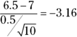 .
. - The conclusion is “reject Ho” because the test statistic is beyond the critical value of
 and hence falls in the “rejection” region.
1 Explain what’s wrong with the following hypotheses: Ho: ![]() versus Ha:
versus Ha: ![]() .
.
2 Suppose that a pizza place claims its average pizza delivery time is 30 minutes, but you believe it takes longer than that. Your sample of 10 pizzas has an average delivery time of 40 minutes. Assume that the population standard deviation is 15 minutes and the times have a normal distribution. Use ![]() .
.
- What are your null and alternative hypotheses?
- What is the critical value?
- What is the test statistic?
- What is the conclusion?
3 Suppose that a sports reporter claims the average football game lasts 3 hours, and you believe it’s more than that. Your random sample of 35 games has an average time of 3.25 hours. Assume that the population standard deviation is 1 hour. Use ![]() . What do you conclude?
. What do you conclude?
4 Show how you get critical values of 1.65, ![]() , and
, and ![]() for a right-tailed, left-tailed, and two-tailed hypothesis test (use
for a right-tailed, left-tailed, and two-tailed hypothesis test (use ![]() and assume a large sample size).
and assume a large sample size).
Testing a Hypothesis about a Population Mean
It is not always the case that ![]() is known or the population has a normal distribution or n is large enough to the use the central limit theorem (CLT). The formula for the test statistic for one population mean in those cases is
is known or the population has a normal distribution or n is large enough to the use the central limit theorem (CLT). The formula for the test statistic for one population mean in those cases is  . Here, s is the sample standard deviation. To calculate it, you
- Calculate the sample mean,
 , and use the given population standard deviation, s. Let n represent the sample size.
 - Calculate the standard error,
 . Save your answer.
 - Find the sample mean minus
 .
. - Divide your result from Step 3 by the standard error you find in Step 2.
Compare your test statistic to the critical value(s) from the t-distribution with ![]() degrees of freedom, as described in Chapter 8. Use the t-table (see the Appendix). If
degrees of freedom, as described in Chapter 8. Use the t-table (see the Appendix). If ![]() is unknown, or the sample size is small, use the sample standard deviation, s, instead of
is unknown, or the sample size is small, use the sample standard deviation, s, instead of ![]() and use the t-distribution with
and use the t-distribution with ![]() degrees of freedom. If your test statistic is beyond the critical value(s), reject Ho; otherwise, fail to reject Ho.
degrees of freedom. If your test statistic is beyond the critical value(s), reject Ho; otherwise, fail to reject Ho.
 To use Z in a hypothesis test, you need either a normal distribution to start with or n to be at least 30 and use the CLT. If the sample size is
 ![]() 30, you can use the t-distribution. In this case, the test is called a t-test.
30, you can use the t-distribution. In this case, the test is called a t-test.
See the following for an example of setting up a t-test for the mean.
Q. Suppose that you hear a claim that the average score on a national exam is 78. You think the average is higher than that, and your sample of 100 students produces an average of 81.
- Set up your null and alternative hypotheses.
- Find the critical value when
 .
.
A. Setting up the hypotheses correctly is critical to your success with hypothesis tests.
- In this case, you have Ho:
 versus Ha:
  . Note: 81 is a sample statistic and doesn’t belong in Ho or Ha. You want to show that the mean is higher than the claim, so the alternative has a “
 ” sign. You’re conducting a right-tailed test.
 - The critical value is
 . Here’s how you get it: We use Table 13-1 here because n = 100 is so large that the t table and Z-table would give the same values.
5 Conduct the hypothesis test Ho: ![]() versus
versus ![]() , where
, where ![]() ,
, ![]() , and
, and ![]() . Use
. Use ![]() .
.
6 Conduct the hypothesis test Ho: ![]() versus Ho:
versus Ho: ![]() , where
, where ![]() ,
, ![]() , and
, and ![]() . Use
. Use ![]() .
.
7 Conduct the hypothesis test Ho: ![]() versus Ha:
versus Ha: ![]() , where
, where ![]() ,
, ![]() , and
, and ![]() . Use
. Use ![]() .
.
8 Suppose that your critical value for a left-tailed hypothesis test is ![]() . For what values of the test statistic would you reject Ho?
. For what values of the test statistic would you reject Ho?
Testing a Hypothesis about a Population Proportion
You use a population proportion hypothesis test when the variable is categorical (such as gender, political party, support/oppose, and so on) and you want to study only one population or group (such as all U.S. citizens or all registered voters). The test looks at the percentage (p) of individuals in the population that have a certain characteristic; for example, the percentage of households that have cellphones. The null hypothesis is Ho: ![]() , where
, where ![]() is a certain value. For example, if the claim is that 20 percent of homes have cellphones,
is a certain value. For example, if the claim is that 20 percent of homes have cellphones, ![]() is 0.20. The alternative hypothesis is one of the following:
is 0.20. The alternative hypothesis is one of the following: ![]() ,
, ![]() , or
, or ![]() .
.
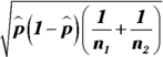
The formula for the test statistic for a single proportion is  . To find it, follow these steps:
- Calculate the sample proportion,
 , by taking the number of people in the sample who have the characteristic of interest and dividing by n, the sample size.
 - Calculate the standard error,
 . Save your answer.
 - Take the sample proportion minus
 .
. - Divide your result from Step 3 by your result from Step 2.
Compare your test statistic to the critical value that you previously set. If the test statistic is beyond the critical value(s), reject Ho.
See the following for an example of setting up and conducting a hypothesis test for a proportion.
Q. Suppose that a political candidate claims the percentage of uninsured drivers is 30 percent, but you believe the percentage is more than 30.
- Set up your null and alternative hypotheses.
- Find the critical value(s), assuming
 and you have a large sample size.
A. First, make sure you can identify that this is a hypothesis test about a proportion. It has a claim that’s being challenged or tested, and the claim is about a percentage (or proportion). That’s how you know.
- The claim is that
 , so you put that into the null hypothesis. The alternative of interest is the one where the percentage is actually more (
 ) than 30. So you have Ho:
  versus Ha:
  .
. - The critical value is
 . Here’s how you get it: Using the Z-table (see the Appendix), the area beyond the critical value must be 0.05. (In this case, beyond means “above,” because you run a right-tailed test.) The Z-table uses percentiles; because 0.05 of the area is above your value, 0.95 must be below it. So look up the 95th percentile on the Z-table in the appendix to find the standard score. It is
  . Or you can just use Table 13-1 because this problem uses 0.05, which just so happens to be included on it; you will also get
  .
.
9 Carry out the hypothesis test of Ho: ![]() versus Ha:
versus Ha: ![]() , where
, where ![]() and
and ![]() . Use
. Use ![]() .
.
10 Carry out the hypothesis test of ![]() versus
versus ![]() , where
, where ![]() and
and ![]() . Use
. Use ![]() .
.
11 Carry out the hypothesis test of Ho: ![]() versus Ha:
versus Ha: ![]() , with
, with ![]() and
and ![]() , where x is the number of people in the sample that have the characteristic of interest. Use
, where x is the number of people in the sample that have the characteristic of interest. Use ![]() .
.
12 Suppose that you want to test the fairness of a single die, so you concentrate on the proportion of 1s that come up. Write down the null and alternative hypotheses for this test.
Testing for a Difference between Two Population Means
This test is used when the variable is numerical (such as income, cholesterol level, or miles per gallon) and two populations or groups are being compared (such as men versus women, athletes versus nonathletes, or cars versus SUVs). Two separate random samples need to be selected, one from each population, to collect the data needed for this test. The null hypothesis is that the two population means are the same; in other words, their difference is equal to 0. The notation for the hypotheses is Ho: ![]() , where
, where ![]() represents the mean of the first population, and
represents the mean of the first population, and ![]() represents the mean of the second population.
represents the mean of the second population.
The formula for the test statistic comparing two means when both populations are normal (or approximately normal) and both population standard deviations are known is  . To find it, follow these steps:
- Calculate the sample means,
 and
and  , and population standard deviations,
  and
and  , for each sample separately. Let
  and
and  represent the two sample sizes (they need not be equal).
 - Find the difference between the two sample means,
 .
. - Calculate the standard error,
 . Save your answer.
 - Divide your result from Step 2 by your result from Step 3.
Compare your test statistic to the critical value from the Z-distribution (Table 13-1).
If the sample sizes are small and you don’t have a normal distribution and/or the population standard deviations are unknown, you substitute ![]() and
and ![]() with the sample standard deviations
with the sample standard deviations ![]() and
and ![]() and use the t-distribution with
and use the t-distribution with ![]() degrees of freedom (see the t-table in the Appendix). If the test statistic is beyond the critical value(s), you reject Ho.
degrees of freedom (see the t-table in the Appendix). If the test statistic is beyond the critical value(s), you reject Ho.
See the following for an example conducting a hypothesis test for two means.
Q. A teacher instructs two statistics classes with two different teaching methods (Group 1: computer versus Group 2: pencil/paper). She wants to see whether the computer method works better by comparing average final exam scores for the two groups. She selects volunteers to be in each group.
- Has the teacher implemented a right-tailed, left-tailed, or two-tailed test?
- The teacher doesn’t try to control for other factors that can influence her results. Name some of the factors.
- How can she change her study to improve the quality of her results?
A. The teacher uses a test for two population means, because she compares the average exam scores, and exam scores are a quantitative variable.
- She wants to see whether the computer group does better, and she puts these students in Group 1, so she wants to show that the mean of Group 1 is greater than (
 ) Group 2. She implements a right-tailed test.
 - Some other factors include the intelligence level of the students, how comfortable they are with computers, the quality of the teaching activities, the way she writes the test, and so on.
- She can improve her results by randomly assigning the students to groups, which creates a more level playing field, rather than asking for volunteers. She can also match up students according to the variables mentioned in part b and randomly assign one member of each pair to the computer group and the other to the pencil/paper group. This would require a paired t-test to do, which comes up later in this chapter.
13 Conduct the hypothesis test Ho: ![]() versus Ha:
versus Ha: ![]() , where
, where ![]() ,
, ![]() ,
, ![]() ,
, ![]() ,
, ![]() , and
, and ![]() . Use
. Use ![]() .
.
14 Conduct the hypothesis test Ho: ![]() versus Ha:
versus Ha: ![]() , where
, where ![]() ,
, ![]() ,
, ![]() ,
, ![]() ,
, ![]() ,
, ![]() . Use
. Use ![]() .
.
15 Conduct the hypothesis test Ho: ![]() versus Ha:
versus Ha: ![]() , where
, where ![]() ,
, ![]() ,
, ![]() ,
, ![]() ,
, ![]() ,
, ![]() . Use
. Use ![]() .
.
16 Suppose that you conducted a hypothesis test for two means (group one mean minus group two mean) and you reject Ho: ![]() versus Ha:
versus Ha: ![]() . You conclude that the two population means aren’t equal. Can you say a little more? Explain how you can tell from the sign on the test statistic which group probably has the higher mean.
. You conclude that the two population means aren’t equal. Can you say a little more? Explain how you can tell from the sign on the test statistic which group probably has the higher mean.
Testing for a Mean Difference (Paired t-Test)
You use this test when the variable is numerical (such as income, cholesterol level, or miles per gallon) and when you pair up the individuals in the sample in some way (identical twins are often used) or use the same people twice (with a pre- and post-test, for example). Researchers typically use paired tests for medical studies when they test to see whether a certain treatment works, without having to worry about other factors associated with the subjects that may influence the results. For example, you want to compare a new blood pressure drug to an existing one to see whether it does a better job. To make it a fair test, you pair up the people in the study according to their weight, age, fitness level, and severity of blood pressure problems. With these pairing parameters, you can attribute any difference in blood pressure to the drug. (See Chapter 16 for more information on designed experiments like this one.)
You collect the data in pairs, and for each pair, you find the difference between the values. For example, suppose that you have a pair of subjects in the blood pressure test. Suppose that the first person in the pair is in the “current drug” group, and her blood pressure is 190 after the experiment. Suppose that the second person is in the “new drug” group, and her blood pressure is 180 after the experiment. The difference in blood pressures for this pair is ![]() , or
, or ![]() . (That means the new drug drops the blood 10 points more than the current drug for this pair.) You make the same calculations for each pair of subjects in the study.
. (That means the new drug drops the blood 10 points more than the current drug for this pair.) You make the same calculations for each pair of subjects in the study.
The set of all the paired differences becomes your new (single) data set. This test is now the same as a test for a single population mean, and the null hypothesis is that the mean is equal to 0. (The average of all the differences should be 0 if the null hypothesis is true.) The notation for the null hypothesis is Ho: ![]() , where
, where ![]() is the mean of the paired differences.
is the mean of the paired differences.
The mean of the paired differences is different from the difference in the means. For the mean of the paired differences, you pair data, and you look at one set of differences for each pair and find the mean of that single data set. For the difference in the means, you have two different populations, so you have to compare their two means separately (see the section “Testing for a Difference between Two Population Means” earlier in this chapter).
The formula for the test statistic for paired differences is ![]() . To calculate it, run through the following steps:
. To calculate it, run through the following steps:
- For each pair of data, take the first value in the pair minus the second value to find the difference. Think of the differences as your new data set.
- Calculate the mean
 and the standard deviation
  of all the differences. Let n represent the number of differences (or pairs) that you have (not necessarily the number of individuals).
 - Calculate the standard error,
 . Save your answer.
 -
Find
 divided by the standard error from Step 3.
Remember,
 under the assumption that Ho is true.
If the number of pairs (n) is 30 or more, compare your test statistic to the critical value(s) from the standard normal distribution (see the Z-table in the Appendix or Table 13-1 earlier in this chapter). If the number of pairs (n) is less than 30, compare your test statistic to the critical value(s) from the t-distribution with ![]() degrees of freedom (see the t-table in the Appendix). If your test statistic is beyond the critical value(s), reject Ho. If not, fail to reject Ho.
degrees of freedom (see the t-table in the Appendix). If your test statistic is beyond the critical value(s), reject Ho. If not, fail to reject Ho.
See the following for an example involving a matched-pairs test.
Q. Suppose that you use a paired t-test using matched pairs to find out whether a certain weight-loss method works. You measure the participants’ weights before and after the study, and you take weight before minus weight after as your pairs of data.
- If you want to show that the program works, what’s your Ha?
- Explain why measuring the same participants both times rather than measuring two different groups of people (those on the program compared to those not) makes this study much more credible.
A. The signs on the differences are important when making comparisons. If you subtract two numbers and get a positive result, that means the first number is larger than the second. If the result is negative, the second is larger than the first.
- If the program works, the weight loss (weight before minus weight after) has to be positive. So you have Ho:
 versus Ha:
  .
. - If you use two different groups of people, you introduce other variables that can account for the weight differences. Using the same people cuts down on unwanted variability by controlling for possible confounding variables.
Note: If you switch the data around and take weight after minus weight before, you have to switch the sign in the alternative hypothesis to be ![]() (less than). Most people like to use positive values, and greater-than signs (
(less than). Most people like to use positive values, and greater-than signs (![]() ) produce them. If you have a choice, always order the groups so the one that may have the higher average is Group 1.
) produce them. If you have a choice, always order the groups so the one that may have the higher average is Group 1.
17 Conduct the hypothesis test Ho: ![]() versus Ha:
versus Ha: ![]() , where
, where ![]() ,
, ![]() , and
, and ![]() . Use
. Use ![]() .
.
18 Conduct the hypothesis test Ho: ![]() versus Ha:
versus Ha: ![]() , where
, where ![]() ,
, ![]() , and
, and ![]() . Use
. Use ![]() .
.
Testing a Hypothesis about Two Population Proportions
You use this test when the variable is categorical (such as smoker/nonsmoker, political party, support/oppose an opinion, and so on) and when you want to know the percentage of individuals with a certain characteristic (such as the percentage of smokers). In this case, you compare two populations or groups (such as men versus women or Democrats versus Republicans). To conduct this test, you need to select two separate random samples — one from each population. The null hypothesis is that the two population proportions are the same; in other words, their difference is equal to 0. The notation for the null hypothesis is Ho: ![]() , where
, where ![]() is the percentage from the first population and
is the percentage from the first population and ![]() is the percentage from the second population.
is the percentage from the second population.
The formula for the test statistic comparing two proportions is  . To find it, follow these steps:
- Calculate the sample proportions
 and
and  for each sample. Let
  and
and  represent the two sample sizes (they need not be equal).
 - Calculate the overall sample proportion,
 , which is the total number of individuals from both samples who have the characteristic of interest divided by the total number of individuals from both samples
  .
. - Find the difference between the two sample proportions,
 .
. - Calculate the standard error,
 . Save your answer.
 - Divide your result from Step 3 by your result from Step 4.
Compare your test statistic to the critical value that you previously set. If the test statistic is beyond the critical value(s), reject Ho. If not, fail to reject Ho. In most cases, the critical value will be on the Z-distribution because the sample sizes will be large in these situations. To be sure, check that ![]() and
and ![]() are both at least 10.
are both at least 10.
See the following for an example of setting up a hypothesis test for two proportions.
Q. Suppose that you want to test whether there’s a higher percentage of males who are Democrat than females who are Democrat.
- Write down your null and alternative hypotheses.
- Explain why it doesn’t matter what the actual percentage of Democrats is for males or females.
A. Your two populations are males and females, and you compare the percentage of Democrats in each group. This means ![]() equals the percentage of all males who are Democrat, and
equals the percentage of all males who are Democrat, and ![]() equals the percentage of all females who are Democrat.
equals the percentage of all females who are Democrat.
- Your Ho is that the percentages are the same
 versus the Ha that
  (because you want to see whether the percentage of males is higher than the percentage of females).
 - Your only concern should be the difference in the percentage of Democrats for males and females and whether the difference is 0. A zero differential can happen in many ways; for example, both genders have about 40 percent Democrats, or both have 80 percent Democrats. The actual values of the proportions don’t matter when you look at their differences.
Note: Saying Ho: ![]() is the same as saying Ho:
is the same as saying Ho: ![]() . Take the first equation and subtract
. Take the first equation and subtract ![]() from each side. The second version gives you a number to put in the null hypothesis (0), which is nice. That’s because if the proportions are equal, their difference has to be 0.
from each side. The second version gives you a number to put in the null hypothesis (0), which is nice. That’s because if the proportions are equal, their difference has to be 0.
19 Conduct the hypothesis test Ho: ![]() versus Ha:
versus Ha: ![]() , where
, where ![]() ,
, ![]() ,
, ![]() ,
, ![]() ,
, ![]() . Use
. Use ![]() .
.
20 Conduct the hypothesis test Ho: ![]() versus Ha:
versus Ha: ![]() , where
, where ![]() ,
, ![]() ,
, ![]() ,
, ![]() . Use
. Use ![]() .
.
Answers to Problems in Testing Hypotheses
1 You see ![]() in both hypotheses, which is wrong. The null and alternative hypotheses make statements about the population parameter, not about the sample statistic.
in both hypotheses, which is wrong. The null and alternative hypotheses make statements about the population parameter, not about the sample statistic.
 Instructors get really bent out of shape when they see this kind of mistake, so avoid it at all costs. Always keep sample statistics like
 ![]() and
and ![]() out of Ho and Ha. Use population parameters like
out of Ho and Ha. Use population parameters like ![]() and p instead.
and p instead.
2 The process of doing a hypothesis test in full requires several steps: setting up the hypotheses, finding the critical value, calculating the test statistic, and making the decision.
- The claim is that the average pizza delivery time is 30 minutes, but you believe it takes longer than that. This means that Ho is
 and Ha is
  .
. - The critical value is 1.96 looking at Table 13-1 because
 and it’s a “
 ” alternative hypothesis, Ha.
 - Your sample of 10 pizzas has an average delivery time of 40 minutes. Assume that the population standard deviation is 15 minutes and the times have a normal distribution. That means the test statistic is
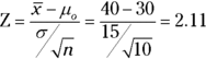 .
. - The conclusion is reject Ho because the test statistic 2.11 is
 1.96. The average pizza delivery time is likely to be more than 30 minutes based on these data.
Make sure you can identify these problems out of context — in other words, when the problems are all mixed up on an exam. You may want to copy some problems, mark where they come from, mix them up, and try to solve them. Also, as you go through the problems in this workbook, always think about how to recognize the types of problems in a test situation and how to approach them. I give you clues to look for; write them down in a quick outline to help you study.
3 Because the claim is that the average football game lasts 3 hours, and you believe it’s more than that, the hypotheses are Ho: ![]() and Ha:
and Ha: ![]() . Your random sample of 35 games has an average time of 3.25 hours, and the population standard deviation is 1 hour so the test statistic is
. Your random sample of 35 games has an average time of 3.25 hours, and the population standard deviation is 1 hour so the test statistic is 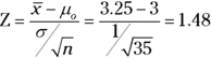 . Using
 ![]() , the critical value is 1.96 from the Z-distribution so the conclusion is fail to reject Ho because the test statistic is less than the critical value. You can’t say with these data that the average football game lasts more than 3 hours.
, the critical value is 1.96 from the Z-distribution so the conclusion is fail to reject Ho because the test statistic is less than the critical value. You can’t say with these data that the average football game lasts more than 3 hours.
4 In a right-tailed test, Ha has a greater-than sign (![]() ) in it. Your critical value on the Z-distribution is 1.64, because the probability of being below 1.64 is equal to 0.95 (see Table 13-1 earlier in this chapter), and the probability of being beyond (in this case, “above”) 1.64 is
) in it. Your critical value on the Z-distribution is 1.64, because the probability of being below 1.64 is equal to 0.95 (see Table 13-1 earlier in this chapter), and the probability of being beyond (in this case, “above”) 1.64 is ![]() . If you run a left-tailed test (Ha has a less-than [
. If you run a left-tailed test (Ha has a less-than [![]() ] sign in it), your critical value is
] sign in it), your critical value is ![]() , because the area beyond (in this case, “below”) –1.64 is 0.05. If you run a two-tailed test (Ha has a not-equal-to sign
, because the area beyond (in this case, “below”) –1.64 is 0.05. If you run a two-tailed test (Ha has a not-equal-to sign ![]() in it), you have two critical values — one positive and one negative — and the total area beyond them (in both directions) is 0.05. That means the area above the positive one is
in it), you have two critical values — one positive and one negative — and the total area beyond them (in both directions) is 0.05. That means the area above the positive one is ![]() , and the area below the negative one is 0.025. The critical values in that case are
, and the area below the negative one is 0.025. The critical values in that case are ![]() , as seen in Table 13-1.
, as seen in Table 13-1.
5 You have a right-tailed test for one population mean with ![]() ,
, ![]() ,
, ![]() , and
, and ![]() . The test statistic is
. The test statistic is 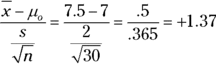 . The critical value for this right-tailed test with
 ![]() is
is ![]() (see t-table in the appendix with 29 degrees of freedom, column for .01.). Conclusion: You shouldn’t reject Ho, because the test statistic is less than the critical value. Interpretation: According to your data, you don’t have enough evidence to say the mean is more than 7.
(see t-table in the appendix with 29 degrees of freedom, column for .01.). Conclusion: You shouldn’t reject Ho, because the test statistic is less than the critical value. Interpretation: According to your data, you don’t have enough evidence to say the mean is more than 7.
Don’t stop with the statistically correct conclusion: reject Ho or fail to reject Ho. Always go back to the question and try to answer it in the context of the problem as best as you can. Your instructor will love you for it.
6 You have a two-tailed test for one population mean with ![]() ,
, ![]() ,
, ![]() , and
, and ![]() . The test statistic is
. The test statistic is  . The critical values for this two-tailed test with
 ![]() are
are ![]() and
and ![]() (see Table 13-1 since the t-distribution is about the same as the Z-distribution when n is 100.) Conclusion: You shouldn’t reject Ho, because the test statistic is between rather than beyond the critical values. Interpretation: You don’t have enough evidence to say that the mean for this population is anything but 75.
(see Table 13-1 since the t-distribution is about the same as the Z-distribution when n is 100.) Conclusion: You shouldn’t reject Ho, because the test statistic is between rather than beyond the critical values. Interpretation: You don’t have enough evidence to say that the mean for this population is anything but 75.
When doing problems involving hypothesis tests, I recommend you immediately write down what type of test you have and what the given information is, as I do in these solutions. It helps your instructor see where you’re going, and it helps you keep it all straight.
7 You have a right-tailed test for one population mean with ![]() ,
, ![]() ,
, ![]() , and
, and ![]() . Notice the sample size is too small to use a Z-distribution, so you have to use the t-distribution. Instructors typically have you use the p-value approach to solving problems involving the t-distribution, but in this case, I want to walk you through one example where you use the critical method (so bear with me!).
. Notice the sample size is too small to use a Z-distribution, so you have to use the t-distribution. Instructors typically have you use the p-value approach to solving problems involving the t-distribution, but in this case, I want to walk you through one example where you use the critical method (so bear with me!).
The degree of freedom for your t-distribution is ![]() , so you can denote this as
, so you can denote this as ![]() . The test statistic is
. The test statistic is  . The critical value for this right-tailed test with
 ![]() is 1.833 on the
is 1.833 on the ![]() distribution. Here’s why: Because this is a right-tailed test, the area beyond (in this case, “above”) the critical value must be
distribution. Here’s why: Because this is a right-tailed test, the area beyond (in this case, “above”) the critical value must be ![]() , which means the area above it must be .05. Find column .05 and the row for 9 degrees of freedom. You find 1.833, so you have your critical value (whew!). Conclusion: You shouldn’t reject Ho, because the test statistic (0.53) isn’t beyond the critical value. Interpretation: You don’t have enough evidence to say that the mean is more than 100.
, which means the area above it must be .05. Find column .05 and the row for 9 degrees of freedom. You find 1.833, so you have your critical value (whew!). Conclusion: You shouldn’t reject Ho, because the test statistic (0.53) isn’t beyond the critical value. Interpretation: You don’t have enough evidence to say that the mean is more than 100.
8 Anything beyond the critical value leads to a rejection of Ho. In this case, the critical value is ![]() , so beyond means “less than”; therefore, any test statistic that comes in less than
, so beyond means “less than”; therefore, any test statistic that comes in less than ![]() leads you to reject Ho.
leads you to reject Ho.
9 You have a right-tailed test for one population proportion, with ![]() ,
, ![]() ,
, ![]() , and
, and ![]() .
.
The test statistic is 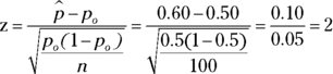 . The critical value for this right-tailed test with
 ![]() is
is ![]() (see Table 13-1). Conclusion: You should reject Ho, because the test statistic is beyond the critical value. Interpretation: According to your data, the proportion of people in the population who have the characteristic of interest is more than 0.50.
(see Table 13-1). Conclusion: You should reject Ho, because the test statistic is beyond the critical value. Interpretation: According to your data, the proportion of people in the population who have the characteristic of interest is more than 0.50.
Always use the decimal version of p when you work with hypothesis tests for one or two proportions. The formulas don’t work if you use percents.
10 You have a left-tailed test for one population proportion, with ![]() ,
, ![]() ,
, ![]() , and
, and ![]() .
.
The test statistic is  . The critical value for this left-tailed test with
 ![]() is
is ![]() (see Table 13-1). Conclusion: You should reject Ho, because the test statistic is beyond the critical value. Interpretation: According to your data, the proportion of people in the population who have the characteristic of interest is less than 0.5.
(see Table 13-1). Conclusion: You should reject Ho, because the test statistic is beyond the critical value. Interpretation: According to your data, the proportion of people in the population who have the characteristic of interest is less than 0.5.
11 You have a two-tailed test for one population proportion, with ![]() ,
, ![]() ,
, ![]() , and
, and ![]() . The sample proportion,
. The sample proportion, ![]() , is the number of people in the sample who have the characteristic of interest divided by n, so in this case,
, is the number of people in the sample who have the characteristic of interest divided by n, so in this case, ![]() . The test statistic is
. The test statistic is 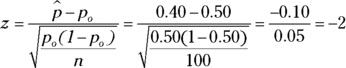 . The critical values for this two-tailed test with
 ![]() are
are ![]() and
and ![]() (see Table 13-1). Conclusion: You shouldn’t reject Ho, because the test statistic is between rather than beyond the critical values. Interpretation: You don’t have enough evidence to say that the proportion of this population who fall in the group of interest is anything but 0.50.
(see Table 13-1). Conclusion: You shouldn’t reject Ho, because the test statistic is between rather than beyond the critical values. Interpretation: You don’t have enough evidence to say that the proportion of this population who fall in the group of interest is anything but 0.50.
12 If the die is fair, each face should show up one-sixth of the time. If you let p equal the proportion of times this die will show a 1, you have Ho: ![]() . The alternative is that the coin isn’t fair, so either
. The alternative is that the coin isn’t fair, so either ![]() or
or ![]() fit that case, which means you have Ha:
fit that case, which means you have Ha: ![]() .
.
13 You have a left-tailed test for two population means with ![]() ,
, ![]() ,
, ![]() ,
, ![]() ,
, ![]() ,
, ![]() , and
, and ![]() . The test statistic is
. The test statistic is 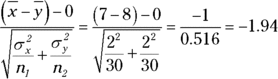 . The critical value for this left-tailed test with
 ![]() is
is ![]() (see Table 13-1). Conclusion: You shouldn’t reject Ho, because the test statistic isn’t beyond the critical value. Interpretation: According to your data, you can’t say the difference in the means of these two populations is less than 0 (indicating no statistically significant difference between the means of these two populations).
(see Table 13-1). Conclusion: You shouldn’t reject Ho, because the test statistic isn’t beyond the critical value. Interpretation: According to your data, you can’t say the difference in the means of these two populations is less than 0 (indicating no statistically significant difference between the means of these two populations).
If you use ![]() in Question 13, the critical value is
in Question 13, the critical value is ![]() , and the test statistic of
, and the test statistic of ![]() is very close to this. You still can’t reject Ho, but you can argue that the close number is a marginal result. The p-value approach (Chapter 14) helps solve the problem of getting different conclusions when you use different
is very close to this. You still can’t reject Ho, but you can argue that the close number is a marginal result. The p-value approach (Chapter 14) helps solve the problem of getting different conclusions when you use different ![]() levels. It allows you to report the strength of your test statistic and to let other people decide for themselves whether the info is enough to reject Ho.
levels. It allows you to report the strength of your test statistic and to let other people decide for themselves whether the info is enough to reject Ho.
14 You have a right-tailed test for two population means, with ![]() ,
, ![]() ,
, ![]() ,
, ![]() ,
, ![]()
![]() , and
, and ![]() .
.
The test statistic is  . The critical value for this right-tailed test with
 ![]() is
is ![]() (see Table 13-1). Conclusion: You should reject Ho, because the test statistic is beyond the critical value. Interpretation: According to your data, the difference in the means of these two populations is greater than 0 (indicating a statistically significant difference between the means of these two populations).
(see Table 13-1). Conclusion: You should reject Ho, because the test statistic is beyond the critical value. Interpretation: According to your data, the difference in the means of these two populations is greater than 0 (indicating a statistically significant difference between the means of these two populations).
15 This is the same hypothesis test as Question 14, except you run a two-tailed test rather than a right-tailed test. Notice that Ho and Ha appear different from usual in this problem, but notice that Ho: ![]() is the same as Ho:
is the same as Ho: ![]() (just subtract
(just subtract ![]() from each side of the original equation). This is another way your professor may write these hypotheses, so be ready for it.
from each side of the original equation). This is another way your professor may write these hypotheses, so be ready for it.
To work the problem, note that, again, you have a two-tailed test for two population means, with ![]() ,
, ![]() ,
, ![]() ,
, ![]() ,
, ![]() ,
, ![]() , and
, and ![]() . Again, the test statistic is 2.02. However, the critical values for this (now) two-tailed test with
. Again, the test statistic is 2.02. However, the critical values for this (now) two-tailed test with ![]() are
are ![]() and
and ![]() (see Table 13-1). Conclusion: You should still reject Ho, because the test statistic is beyond the critical value, but it isn’t as far beyond the critical value as it is in Question 14. Interpretation: According to your data, the difference in the means of these two populations is greater than 0, indicating a statistically significant difference between the means of these two populations. (And because the difference is positive, you can say that the first population has a larger mean than the second population.)
(see Table 13-1). Conclusion: You should still reject Ho, because the test statistic is beyond the critical value, but it isn’t as far beyond the critical value as it is in Question 14. Interpretation: According to your data, the difference in the means of these two populations is greater than 0, indicating a statistically significant difference between the means of these two populations. (And because the difference is positive, you can say that the first population has a larger mean than the second population.)
Two-tailed tests require you to split the ![]() level in half. The half level means the probability of being outside the critical values is cut in half for each side, making the critical values push out farther on each edge. In other words, if you can make a goal by going to either end of the field, you have to push both goal posts out farther to make up for it. So the result you have with a one-tailed test isn’t as strong when you go to the two-tailed test. A one-tailed test puts all your eggs in one basket. A two-tailed test makes you divide your eggs into two baskets, so to speak.
level in half. The half level means the probability of being outside the critical values is cut in half for each side, making the critical values push out farther on each edge. In other words, if you can make a goal by going to either end of the field, you have to push both goal posts out farther to make up for it. So the result you have with a one-tailed test isn’t as strong when you go to the two-tailed test. A one-tailed test puts all your eggs in one basket. A two-tailed test makes you divide your eggs into two baskets, so to speak.
16 After Ho has been rejected and you conclude that the groups don’t have the same mean, the numerator of your test statistic ![]() tells you which group had the larger mean. If the numerator of your test statistic is positive,
tells you which group had the larger mean. If the numerator of your test statistic is positive, ![]() , which means
, which means ![]() . That means in terms of the populations, the mean of group one (which is
. That means in terms of the populations, the mean of group one (which is ![]() ) is likely to be larger than the mean of group two (which is
) is likely to be larger than the mean of group two (which is ![]() ). If the numerator of your test statistic is negative,
). If the numerator of your test statistic is negative, ![]() , which means
, which means ![]() . That means in terms of the populations, the mean of group one (which is
. That means in terms of the populations, the mean of group one (which is ![]() ) is likely to be smaller than the mean of group two (which is
) is likely to be smaller than the mean of group two (which is ![]() ). Of course, these results all depend on the samples being representative of their populations.
). Of course, these results all depend on the samples being representative of their populations.
17 You have a right-tailed test for the average difference with ![]() ,
, ![]() ,
, ![]() , and
, and ![]() . You do this test the same way you conduct a test for one population mean. The test statistic is
. You do this test the same way you conduct a test for one population mean. The test statistic is  . Because the sample size is under 30, you compare your test statistic to the t-distribution with
 ![]() degrees of freedom, denoted
degrees of freedom, denoted ![]() . On that distribution, 1.27 falls between column .25 and .10. The p-value falls between these numbers. Conclusion: You shouldn’t reject Ho, because the p-value isn’t smaller than .05. Interpretation: According to your data, you can’t say the mean difference for this population is greater than 0 (indicating no statistically significant mean difference for this population).
. On that distribution, 1.27 falls between column .25 and .10. The p-value falls between these numbers. Conclusion: You shouldn’t reject Ho, because the p-value isn’t smaller than .05. Interpretation: According to your data, you can’t say the mean difference for this population is greater than 0 (indicating no statistically significant mean difference for this population).
18 You have the same hypothesis test as Question 17 here, except the sample size is larger for this test. You have a right-tailed test for the average difference with ![]() ,
, ![]() ,
, ![]() , and
, and ![]() .
.
The test statistic is 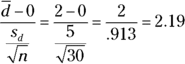 , which is larger than the test statistic in Question 17. Because the sample size is 30 or more, you compare your test statistic to the Z-distribution. The critical value for this right-tailed test with
 ![]() is 1.64. Conclusion: You should reject Ho, because the test statistic is beyond the critical value. Interpretation: According to your data, the mean difference for this population is greater than 0 (indicating a statistically significant and positive mean difference for this population).
is 1.64. Conclusion: You should reject Ho, because the test statistic is beyond the critical value. Interpretation: According to your data, the mean difference for this population is greater than 0 (indicating a statistically significant and positive mean difference for this population).
A larger sample size makes it easier to reject Ho. It makes your test statistic more extreme, which increases its chances of crossing over into the rejection region. And in the case of Question 18, where the sample size goes from 10 to 30, the critical value decreases, because you don’t have to use the t-distribution anymore. Remember, the t-distribution makes you pay a penalty for having less data, and that penalty involves pushing out the tails of the t-distribution so you have to get farther out there to reject Ho. A wider boundary makes it harder to reject Ho. (See Chapter 8 for more on the t-distribution.)
19 You have a right-tailed test for two population proportions with ![]() ,
, ![]() ,
, ![]() ,
, ![]() ,
, ![]() ,
, ![]() .
.
The test statistic is 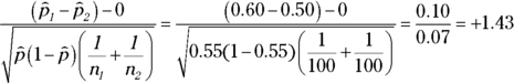 .
.
The critical value for this right-tailed test with ![]() is
is ![]() (see Table 13-1). Conclusion: You shouldn’t reject Ho, because the test statistic isn’t beyond the critical value. Interpretation: According to your data, we can’t say the difference in the proportions for these two populations is greater than 0 (indicating no statistically significant difference between the proportions for these two populations).
(see Table 13-1). Conclusion: You shouldn’t reject Ho, because the test statistic isn’t beyond the critical value. Interpretation: According to your data, we can’t say the difference in the proportions for these two populations is greater than 0 (indicating no statistically significant difference between the proportions for these two populations).
20 You have a two-tailed test for two population proportions with ![]() ,
, ![]() ,
, ![]() . The test statistic is
. The test statistic is  .
.
The critical values for this two-tailed test with ![]() are
are ![]() (see Table 13-1). Conclusion: You should reject Ho, because the test statistic is beyond the critical values. Interpretation: According to your data, the difference in the proportions for these two populations isn’t equal to 0, indicating a statistically significant difference between the proportions for these two populations. (And because the test statistic is negative [taking Group 1 – Group 2], the proportion in the first population who have that characteristic of interest is likely to be lower than the proportion in the second population who have the characteristic of interest.)
(see Table 13-1). Conclusion: You should reject Ho, because the test statistic is beyond the critical values. Interpretation: According to your data, the difference in the proportions for these two populations isn’t equal to 0, indicating a statistically significant difference between the proportions for these two populations. (And because the test statistic is negative [taking Group 1 – Group 2], the proportion in the first population who have that characteristic of interest is likely to be lower than the proportion in the second population who have the characteristic of interest.)