
Chapter 6
Measures of Relative Standing and the Normal Distribution
IN THIS CHAPTER
![]() Working with the normal distribution — frontward and backward
Working with the normal distribution — frontward and backward
![]() Translating to a standard normal (Z) distribution
Translating to a standard normal (Z) distribution
![]() Calculating and interpreting Z-scores
Calculating and interpreting Z-scores
![]() Finding and understanding percentiles for the normal distribution
Finding and understanding percentiles for the normal distribution
This chapter helps you get comfortable with the normal distribution — the most popular distribution in introductory statistics. You practice converting to the standard normal (Z) distribution and interpreting exactly what the distribution means. I show you how to find and interpret percentiles for the normal distribution, and you practice on “backwards normal” problems that instructors like so much (the problems that give you a percent and ask you to find the cutoff point).
Mastering the Normal Distribution
You may have heard of a bell curve. A bell curve describes data from a variable that has an infinite (or very large) number of possible values distributed among the population in a bell shape. This basically means a big group of individuals gravitate near the middle, with fewer and fewer individuals trailing off as you move away from the middle in either direction. Statisticians call a distribution with a bell-shaped curve a normal distribution. You can see a normal distribution’s shape in Figure 6-1.

© John Wiley & Sons, Inc.
FIGURE 6-1: Laypeople call it a bell curve; you call it a normal distribution.
Every normal distribution has certain properties. You can use these properties to determine the relative standing of any particular result on the distribution. The properties of any normal distribution (bell curve) are as follows:
- The shape is symmetric.
- The distribution has a mound in the middle, with tails going down to the left and right.
- The mean is directly in the middle of the distribution. (The mean of the population is designated by the Greek letter
 .)
.) - The mean and the median are the same value because of the symmetry.
- The standard deviation is the distance from the center to the saddle point (the place where the curve changes from an “upside-down-bowl” shape to a “right-side-up-bowl” shape. (The standard deviation of the population is designated by the Greek letter
 .)
.) - About 68 percent of the values lie within one standard deviation of the mean, about 95 percent lie within two standard deviations, and most of the values (99.7 percent or more) lie within three standard deviations by the empirical rule (see Chapter 4). (You practice on the tables in this chapter to get more specific.)
- Each normal distribution has a different mean and standard deviation that make it look a little different from the rest, yet they all have the same bell shape.
See the following for an example of comparing two normal distributions.
 Q. Which of these two normal distributions has a larger standard deviation?


A. The first distribution has a larger standard deviation, because the data are more spread out from the center, and the tails take longer to go down and away.
1 What do you guess are the standard deviations of the two distributions in the previous example problem?
2 Draw a picture of a normal distribution with mean 70 and standard deviation 5.
3 Draw one picture containing two normal distributions. Give each a mean of 70, one a standard deviation of 5, and the other a standard deviation of 10. How do the distributions differ?
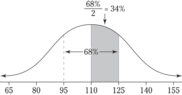
4 Suppose that you have a normal distribution with mean 110 and standard deviation 15.
- About what percentage of the values lie between 110 and 125?
- About what percentage of the values lie between 95 and 140?
- About what percentage of the values lie between 80 and 95?
Finding and Interpreting Standard (Z) Scores
To find, report, and interpret the relative standing of any value on a normal distribution, you need to convert it to what statisticians call a standard score. The Z-formula for standardizing your value looks like this: ![]() .
.
To convert an original score to a standard score:
- Find the mean and the standard deviation of the values you’re working with.
- Take the value you want to convert and subtract the mean.
- Divide your result by the standard deviation.
Standard scores, also known as Z-scores, have a universal interpretation, which is what makes them so great.
 Instructors love to ask you to interpret standard scores. If an instructor gives you a standard score, be ready to interpret it right away. For example, a standard score of
 ![]() on an exam says that the score is two standard deviations above the mean, which is quite good in this case. If you’re measuring times it takes to run around the block, however, a standard score of
on an exam says that the score is two standard deviations above the mean, which is quite good in this case. If you’re measuring times it takes to run around the block, however, a standard score of ![]() would be a bad thing, because your time was two standard deviations above the mean. In this case, a standard score of
would be a bad thing, because your time was two standard deviations above the mean. In this case, a standard score of ![]() would be much better, indicating your time was less than most of the other runners. To interpret a standard score, you don’t need to know the original score, the mean, or the standard deviation. The standard score gives you the relative standing of a value, which, in most cases, is what matters most.
would be much better, indicating your time was less than most of the other runners. To interpret a standard score, you don’t need to know the original score, the mean, or the standard deviation. The standard score gives you the relative standing of a value, which, in most cases, is what matters most.
When your data has a normal distribution, its Z-scores have a special normal distribution — one that has mean 0 and standard deviation 1. This distribution is called the standard normal distribution or the Z-distribution (see Figure 6-2).

© John Wiley & Sons, Inc.
FIGURE 6-2: The standard normal distribution has mean 0 and standard deviation 1.
See the following for an example of interpreting a standard score.
Q. Suppose that you play a round of golf and want to compare your score to the other members of your club population. You find that your score is below the mean.
- What does this tell you about your standard score?
- Is this a good thing or a bad thing?
A. To interpret the standard score, the sign is the first part to look at.
- Falling below the mean indicates a negative standard score.
- Often, being below the mean is a bad thing, but in golf you have an advantage because golf scores measure the number of swings you need to get around the course, and you want to have a low golf score. So being below the mean in this case is a good thing.
5 Exam scores have a normal distribution with mean of 70 and standard deviation of 10. Bob’s score is 80. Find and interpret his standard score.
6 Bob scores 80 on both his math exam (which has a mean of 70 and standard deviation of 10) and his English exam (which has a mean of 85 and standard deviation of 5). Find and interpret Bob’s Z-scores on both exams to let him know which exam (if either) he did better on. Don’t, however, let his parents know; let them think he’s just as good at both subjects.
7 Sue’s math class exam has a mean of 70 with a standard deviation of 5. Her standard score is ![]() . What’s her original exam score?
. What’s her original exam score?
8 Suppose that your score on an exam is directly at the mean. What’s your standard score?
9 Suppose that the weights of cereal boxes have a normal distribution with a mean of 20 ounces and standard deviation of half an ounce. A box that has a standard score of 0 weighs how much?
10 Suppose that you want to put fat Fido on a weight-loss program. Before the program, his weight had a standard score of ![]() compared to dogs of his breed/age, and after the program, his weight has a standard score of
compared to dogs of his breed/age, and after the program, his weight has a standard score of ![]() . His weight before the program was 150 pounds, and the standard deviation for the breed is 5 pounds.
. His weight before the program was 150 pounds, and the standard deviation for the breed is 5 pounds.
- What’s the mean weight for Fido’s breed/age?
- What’s his weight after the weight-loss program?
Knowing Where You Stand with Percentiles
Percentiles are another way to measure where you stand in a data set. If you come in at the 90th percentile, for example, 90 percent of the values are below you (and 10 percent are above you). In general, being at the kth percentile means k percent of the data lie below that point and ![]() percent lie above it.
percent lie above it.
To calculate a percentile when the data has a normal distribution:
- Convert the original score to a standard score by taking the original score minus the mean and dividing by the standard deviation (in other words, use the Z-formula).
-
Use the Z-table (in the Appendix) to find the corresponding percentile for the standard score.
The values on the Z-table have a standard normal distribution (the special normal distribution with a mean of 0 and standard deviation of 1). The distribution is made up entirely of standard scores, or Z-scores, and is often called the Z-distribution.
See the following for an example of finding a percentile for a normal distribution.
Q. Weights for single dip ice-cream cones at Adrian’s have a normal distribution with a mean of 8 ounces and standard deviation of one-quarter ounce. Suppose that your ice-cream cone weighs 8.5 ounces. What percentage of cones are smaller than yours?
A. Your cone weighs 8.5 ounces, and you want the corresponding percentile. Before you can use the Z-table to find that percentile, you need to standardize the 8.5 — in other words, run it through the Z-formula. This gives you ![]() , so the Z-score for your ice-cream cone is
, so the Z-score for your ice-cream cone is ![]() . Now you use the table and find that the
. Now you use the table and find that the ![]() in the standard score column corresponds with 97.72 percent. Your ice-cream cone is at the 97.72rd percentile, and 97.72 percent of the other single dip cones at Adrian’s are smaller than yours. Lucky you!
in the standard score column corresponds with 97.72 percent. Your ice-cream cone is at the 97.72rd percentile, and 97.72 percent of the other single dip cones at Adrian’s are smaller than yours. Lucky you!
11 Bob’s commuting times to work have a normal distribution with a mean of 45 minutes and standard deviation of 10 minutes.
- What percentage of the time does Bob get to work in 30 minutes or less?
- Bob’s workday starts at 9 a.m. If he leaves at 8 a.m., how often is he late?
12 Times to complete a statistics exam have a normal distribution with a mean of 40 minutes and standard deviation of 6 minutes. Deshawn’s time comes in at the 90th percentile. What percentage of the students are still working on their exams when Deshawn leaves?
13 Suppose that your exam score has a standard score of 0.90. Does this mean that 90 percent of the other exam scores are lower than yours?
14 If a baby’s weight is at the median, what’s her percentile?
15 Clint sleeps an average of 8 hours per night with a standard deviation of 15 minutes. What’s the chance he will sleep less than 7.5 hours tonight?
16 Suppose you know that Bob’s test score is above the mean, but he doesn’t remember by how much. At least how many students must score lower than Bob?
Finding Probabilities for a Normal Distribution
To find probabilities for any normal distribution:
- Convert the values to standard scores, using the Z-formula.
- Look up their percentiles, using the Z-table (in the Appendix).
- Use those percentiles (by adding them, subtracting them, taking them as they are, or taking 100 percent minus the percentile in the Z-table) to get your final answer.
In this section, you practice each technique.
 You may come across many different types of tables for the Z-distribution; the Z-table I use (in the Appendix) is a common one, but the Z-table in your textbook may appear different and may even contain more decimal places than mine. My Z-table gives you the percentile, or area below a given value, not the area from the mean out to the value (as is done with the empirical rule [refer to Chapter 4] and some other types of Z-tables). So whether you should add or subtract probabilities after you find them depends on whether you’re using the empirical rule (Chapter 4) or the Z-table (this is typically the case with most textbooks as well). Always make sure you understand exactly how your tables work before you attempt to solve probability problems.
See the following for an example of finding the probability of being between two values on a normal distribution.
Q. The weights of single dip ice-cream cones at Bob’s ice cream parlor have a normal distribution with a mean of 8 ounces and standard deviation of one-half ounce (0.5 ounces). What’s the chance that an ice-cream cone weighs between 7 and 9 ounces?
A. In this case, you want the area between two values, so you convert each of them to Z-scores, find their percentiles on the Z-table, and subtract those percentiles taking the largest one minus the smallest one. Nine ounces becomes ![]() . The corresponding percentile for
. The corresponding percentile for ![]() is 97.73. Seven ounces becomes
is 97.73. Seven ounces becomes ![]() , which has a corresponding percentile of 2.28 from the Z-table. Subtracting these percentiles gives you the area between:
, which has a corresponding percentile of 2.28 from the Z-table. Subtracting these percentiles gives you the area between: ![]() .
.
17 Bob’s commuting times to work have a normal distribution with a mean of 45 minutes and standard deviation of 10 minutes. How often does Bob get to work in 30 to 45 minutes?
18 The times taken to complete a statistics exam have a normal distribution with a mean of 40 minutes and standard deviation of 6 minutes. What’s the chance of Deshawn completing the exam in 30 to 35 minutes?
19 Times until service at a restaurant have a normal distribution with mean of 10 minutes and standard deviation of 3 minutes. What’s the chance of it taking longer than 15 minutes to get service?
20 At the same restaurant as in Question 19 with the same normal distribution, what’s the chance of it taking no more than 15 minutes to get service?
21 Clint, obviously not in college, sleeps an average of 8 hours per night with a standard deviation of 15 minutes. What’s the chance of him sleeping between 7.5 and 8.5 hours on any given night?
22 One state’s annual rainfall has a normal distribution with a mean of 100 inches and standard deviation of 25 inches. Suppose that corn grows best when the annual rainfall is between 100 and 150 inches. What’s the chance of achieving this amount of rainfall?
Finding the Percentile (Backwards Normal)
Now you’re ready to face the situation that students seem to dread the most and that professors seem sure to ask about. You’re given the percentage of values that lie at the bottom or the top of the normal distribution, and you need to find the cutoff point that goes along with that percent. Want the good news? Backwards normal problems aren’t as bad as they may seem, as long as you establish a pattern by which you can identify them when they come up and then work through them systematically. This section helps you do just that.
You know you have a backwards normal problem when you have a normal distribution, you are given a percentage of values above or below a cutoff point, and you need to find that cutoff point. To break out of backwards-normal purgatory:
- Identify a given percentile, using the given information.
- Find the percentile’s corresponding standard score, using the Z-table (in the Appendix).
-
Convert the Z-score back to original units.
To do this conversion, you can either take the Z-formula, put in the items you know (the mean, standard deviation, and value for z), and solve it for x, or you can use a formula that’s already done that solving for you. I call this the Z-formula solved for x:
 . It’s the same as the Z-formula, except it has already been solved for x by cross multiplying by the standard deviation and adding the mean to both sides.
It’s always a good idea to have the Z-formula and the Z-formula solved for x handy. That way you don’t have to do all the algebra yourself if your instructor asks you to find x given a percentile. And you’ll know right away which formula to use in which situation. If you’re given x and asked for the percent, use the Z-formula. If you’re given the percent and asked to find x, use the Z-formula solved for x. (Note: In the remaining problems, I use the Z-formula solved for x to solve backwards normal problems.)
To do a backwards normal problem, you literally work backward from how you find probabilities for the normal distribution. See the following for an example of a backwards normal problem, or reverse normal problem (as we call them in the business).
Q. Racehorses race around the track in a qualifying round according to a normal distribution with a mean of 120 seconds and standard deviation of 5 seconds. The top 10 percent of the times qualify; the rest don’t. What’s the cutoff time for qualifying?
A. You may think you need to find the 90th percentile, but no. The bigger values for times don’t make the cut, and the smallest 10 percent of the times do make it, so in terms of data on a normal distribution, you know that the percentile of interest is the 10th. Remember that the percentage of times below the cutoff is 10, and the percentage above the cutoff is 90 (that’s how percentiles work). The standard score for the 10th percentile is ![]() , looking at the Z-table. Converting this back to original units, you get
, looking at the Z-table. Converting this back to original units, you get ![]() . So the cutoff time is 113.6 seconds.
. So the cutoff time is 113.6 seconds.
23 Weights have a normal distribution with a mean of 100 and standard deviation of 10. What weight has 60 percent of the values lying below it?
24 Jimmy walks a mile, and his previous times have a normal distribution with a mean of 8 minutes and standard deviation of 1 minute. What time does he have to make to get into his own top 10 percent of his fastest times?
25 The times it takes to complete a statistics exam have a normal distribution with a mean of 40 minutes and standard deviation of 6 minutes. Deshawn’s time falls at the 42nd percentile. How long does Deshawn take to finish her exam?
26 Exam scores for a particular test have a normal distribution with a mean of 75 and standard deviation of 5. The instructor wants to give the top 20 percent of the scores an A. What’s the cutoff for an A?
27 Service call times for one company have a normal distribution with a mean of 10 minutes and standard deviation of 3 minutes. Researchers study the longest 10 percent of the calls to make improvements. How long do the longest 10 percent last?
28 Statcars have a miles per gallon normal distribution with a mean of 75. Twenty percent of the vehicles get more than 100 miles per gallon. What’s the standard deviation?
Answers to Problems in Normal Distribution
1 In the first normal distribution, most of the data falls between 10 and 70, each within 3 times 10 units of the mean (40), so you can assume that the standard deviation is around 10. You can also see that the saddle point (the place where the picture changes from an upside-down bowl to a right-side-up bowl) occurs about 10 units away from the mean of 40, which means the standard deviation is around 10. In the second normal distribution, the saddle point occurs about 5 units from the mean, so the standard deviation is at about 5. Notice also that most all the data lies within 15 units of the mean, which is 3 standard deviations.
2 See the following figure. Check that you have saddle points at 65 and 75.

3 See the following figure. A graph with a standard deviation of 5 is taller and thinner than a graph whose standard deviation is 10. The normal distribution with a standard deviation of 10 is more spread out and flatter looking than the normal distribution with a standard deviation of 5, which looks more squeezed together close to the mean (which it is).

A normal distribution that looks flatter actually has more variability than one that goes from low to high to low as you look from left to right, because you measure variability by how far away the values are from the middle; more data close to the middle means low variability, and more data farther away means less variability. This characteristic differs from what you see on a graph that shows data over time (time series or line graphs). On the time graphs, a flat line means no change over time, and going from low to high to low means great variability.
4 A picture is worth a thousand points here (along with the empirical rule). See the following figure.

- For the two values 110 and 125, 125 is one standard deviation above the mean, and about 68 percent of the values lie within one standard deviation of the mean (on both sides of it). So the percentage of values between 110 and 125 is half of 68 percent, which is 34 percent. The following figure illustrates this point.
- For the two values 95 and 140, 95 is one standard deviation below the mean (110), so that distance covers half of the 68 percent again, or 34 percent. To get from 110 to 140, you need to go two standard deviations above the mean. Because about 95 percent of the data lie within two standard deviations of the mean (on both sides of it), from 110 to 140 covers about half of the 95 percent, which is 47.5 percent. Add the 34 and the 47.5 to get 81.5 percent for your approximate answer. See the following figure for an illustration.

- For the two values 80 and 95, 80 is two standard deviations below the mean of 110, which represents
 or 47.5% of the data. And 95 is one standard deviation below 110, which represents
  or 34% of the data. You want the area between these two values, so subtract the percentages:
 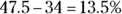 . See the following figure for a visual.
When using the empirical rule to find the percentage between two values, you may have to use a different approach, depending on whether both values are on the same side of the mean or one is above the mean and one below the mean. First, find the percentages that lie between the mean and each value separately. If the values fall on different sides of the mean, add the percentages together. When they appear on the same side of the mean, subtract their percentages (largest minus smallest, so the answer isn’t negative). Or, better yet, draw a picture to see what you need to do.
5 The following figure shows a picture of this distribution. Take ![]() and divide by 10 to get 1. Bob’s score is one standard deviation above the mean. You can see this on a picture as well, because Bob’s score falls one “tick mark” above the mean on the picture of the original normal distribution.
and divide by 10 to get 1. Bob’s score is one standard deviation above the mean. You can see this on a picture as well, because Bob’s score falls one “tick mark” above the mean on the picture of the original normal distribution.


6 The 80 Bob scores on his math exam converts to a standard score of 1 (see Question 5). The 80 Bob scores on his English exam converts to a standard score of ![]() . His score on the English exam is one standard deviation below the mean, so his math score is better.
. His score on the English exam is one standard deviation below the mean, so his math score is better.
Your actual scores don’t matter; what matters is how you compare to the mean, in terms of number of standard deviations.
7 Here you can use the same formula, ![]() , but you need to plug in different values. You know that the mean is 70 and the standard deviation is 5. You know
, but you need to plug in different values. You know that the mean is 70 and the standard deviation is 5. You know ![]() , but you don’t know x, the original score. So what you have looks like
, but you don’t know x, the original score. So what you have looks like ![]() . Solving for X, you get
. Solving for X, you get ![]() , so
, so ![]() , or
, or ![]() . The answer makes sense because each standard deviation is worth 5, and you start at 70 and go down two of these standard deviations:
. The answer makes sense because each standard deviation is worth 5, and you start at 70 and go down two of these standard deviations: ![]() . So Sue scored a 60 on the test.
. So Sue scored a 60 on the test.
8 A standard score of 0 means your original score is the mean itself, because the standard score is the number of standard deviations above or below the mean. When your score is on the mean, you don’t move away from it at all. Also, in the Z-formula, after you take the value (which is at the mean) and subtract the mean, you get 0 in the numerator, so the answer is 0.
9 Exactly 20 ounces, because a standard score of 0 means the observation is right on the mean.
10 This problem is much easier to calculate if you first draw a picture of what you know and work from there.
- The following figure shows a picture of the situation before and after Fido’s weight-loss program. You know that 150 has a Z-score of
 and the standard deviation is 5, so you have
  . And solving for the mean
  , you calculate
  . The mean weight for his breed/age group is 140 pounds.
 - A Z-score of
 corresponds to a weight 2 standard deviations below the mean of 150, which brings you down to
 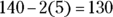 . Fido weighs 130 pounds after the program.

For any problem involving a normal distribution, drawing a picture is the key to success.
11 For this problem, you need to be able to translate the information into the right statistical task.
- Because you want a percentage of time that falls below a certain value (in this case, 30), you need to look for a percentile that corresponds with that value (30). You standardize 30 to get a Z-score of
 by taking 30 minus 45 and then dividing by 10. This means a 30-minute commuting time is well below the mean (so it shouldn’t happen very often). The percentile that corresponds to –1.5, according to the Z-table (see the Appendix), is 6.68, which means Bob gets to work in 30 minutes or less only 6.68 percent of the time.
 -
If Bob leaves at 8 a.m. and is still late for work, his commuting time must be more than 60 minutes (a time that brings him to work after 9 a.m.), so you want the percentage of time that his commute is above 60. Percentiles don’t automatically give you the percentage of data that lies above a given number, but you can still find it. If you know what percentage of the time he gets to work in less than 60 minutes, you can take 100 percent minus that time to get the percentage of time he gets to work in more than 60 minutes. You standardize 60 to get
 and find the percentile that goes with that — 93.32%. Then take
 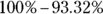 to get 6.68%.
The answer to part b of this question is the same as the answer to part a by symmetry of the normal distribution. Thirty and 30 are both 1.5 standard deviations away from the mean, so the percentage below 30 and the percentage above 60 should be the same.
12 Because Deshawn is at the 90th percentile, 90 percent of the students have exam times lower than hers, which means they all leave before the remaining 10 percent finish. So the answer is 10 percent.
13 No. It means your exam score is 0.90 standard deviations above the mean. You have to look up 0.90 on the Z-table (see the Appendix) to find its corresponding percentile, which is 81.59 percent; therefore, 81.59 percent of the exam scores are lower than yours.
Make sure you keep your units straight; a Z-score between 0 and 1 looks a lot like a percentile, but it isn’t!
14 The median is the value in the middle of the data set; it cuts the data set in half. Half of the data fall below the median, and half rise above it. So the median is at the 50th percentile. (See Chapter 4 for more on the median.)
15 Here’s another way to describe a percentile: the chance of getting a value lower than a certain number. Question 15 uses two different units — hours and minutes — so the first step is to convert everything into the same units. It seems easiest to convert the 15 minutes to hours by using the proportion hours/minutes: ![]() , so
, so ![]() is the standard deviation in minutes. Now you want the probability that X is less than or equal to 7.5, when x has a mean of 8 hours and standard deviation of 0.25 hours. You convert the 7.5 with the Z-formula to get
is the standard deviation in minutes. Now you want the probability that X is less than or equal to 7.5, when x has a mean of 8 hours and standard deviation of 0.25 hours. You convert the 7.5 with the Z-formula to get ![]() .
.
Now look up the percentile because you want the probability of being less than that value. The answer is 2.28 percent (or 0.0228 in decimal form).
Setting up the problem correctly and knowing how to begin is 90 percent of the job. After you set it up, you shouldn’t have a problem working it out. Spend time reading problems and thinking about how to start them for good practice.
16 If Bob’s score is above the mean, his standard score is positive, and the percentage of values below his score is above the 50th percentile. If his score is right at the mean, he scores in the 50th percentile.
17 The following figure shows a picture of the situation. You want the probability that x is between 30 and 45, where x is the commuting time. Converting the 30 to a standard score with the Z-formula, you get ![]() . Forty-five converts to zero because it’s right at the mean. (Note that
. Forty-five converts to zero because it’s right at the mean. (Note that ![]() is 0, and 0 divided by 10 is still 0.) Because you have to find the probability of being between two numbers, you look up each of the percentiles associated with their standard scores on the Z-table (see the Appendix) and subtract their values (largest minus smallest, to avoid a negative answer). Using the Z-table, the percentile for
is 0, and 0 divided by 10 is still 0.) Because you have to find the probability of being between two numbers, you look up each of the percentiles associated with their standard scores on the Z-table (see the Appendix) and subtract their values (largest minus smallest, to avoid a negative answer). Using the Z-table, the percentile for ![]() is 6.68, and the percentile for
is 6.68, and the percentile for ![]() is 50%. Subtracting those gives you
is 50%. Subtracting those gives you ![]() .
.
The reason you subtract the two percentiles when finding the probability of being between two numbers is because the percentile includes all the probability less than or equal to a certain value. You want the probability of being less than or equal to the larger number, but you don’t want the probability of being less than or equal to the smaller number. Subtracting the percentiles allows you to keep the part you want and throw away the part you don’t want.
18 The following figure shows a picture of this situation. You want the probability that x (exam time) is between two values, 30 and 35, on the normal distribution. First, you convert each of the values to standard scores, using the Z-formula. The 30 converts to ![]() (or
(or ![]() ), which is at the 4.46th percentile. The 35 converts to
), which is at the 4.46th percentile. The 35 converts to ![]() (or
(or ![]() ), which is at the 21.19th percentile. To get the probability, or area, between the two values, subtract each of their percentiles — the larger one minus the smaller one — to get
), which is at the 21.19th percentile. To get the probability, or area, between the two values, subtract each of their percentiles — the larger one minus the smaller one — to get ![]() .
.

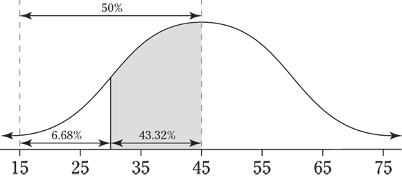
19 You want the probability that X (service time) is more than 15 minutes (see the following figure). In this case, you convert the value to a standard score, find its percentile, and take 100 minus the percentile because you want the percentage that falls above it. Substituting the values, you have ![]() (or 1.7), which is at the 95.54th percentile. The probability you want is
(or 1.7), which is at the 95.54th percentile. The probability you want is ![]() .
.
20 This problem is the exact opposite (or complement) of Question 19. Here, you want the probability that X is no more than 15, which means X is less than or equal to 15. If 4.46 percent (0.0446) is the probability of being more than 15 in Question 19, the probability of being less than or equal to 15 is ![]() , which is 0.9554 or 95.54%.
, which is 0.9554 or 95.54%.
The chance of X being exactly equal to a certain value on a normal distribution is zero, so it doesn’t matter whether you take the probability that x is less than 15 or the probability that x is less than or equal to 15. You get the same answer, because the probability that x equals 15 is zero.
21 For this problem, you need to convert 7.5 and 8.5 to standard scores, look up their percentiles on the Z-table (see Appendix), and subtract them by taking the largest one minus the smallest one. In this case, 7.5 converts to a standard score of ![]() (see the answer to Question 15). Now 8.5 converts to a standard score of
(see the answer to Question 15). Now 8.5 converts to a standard score of ![]() because you have
because you have ![]() . The corresponding percentiles for
. The corresponding percentiles for ![]() and
and ![]() are 2.28 and 97.72, respectively. Subtracting the largest percentile minus the smallest, you get 95.44. Clint has a high chance of sleeping between 7.5 and 8.5 hours on a given night.
are 2.28 and 97.72, respectively. Subtracting the largest percentile minus the smallest, you get 95.44. Clint has a high chance of sleeping between 7.5 and 8.5 hours on a given night.
Practice wording problems in different ways, and pay attention to homework and in-class examples worded differently, too. You don’t want to be thrown off in an exam situation. Your instructor may have certain ways of her own to word questions. This comes through in her examples in class and on homework questions.
22 Here you want the probability that x (annual rainfall) is between 150 and 100, so convert both numbers to standard scores with the Z-formula, look up their percentiles, and subtract (take the biggest minus the smallest). The 150 converts to ![]() and has a percentile of 97.72. The 100 converts to 0 and has a percentile of 50. Subtract the percentiles to get the area between them:
and has a percentile of 97.72. The 100 converts to 0 and has a percentile of 50. Subtract the percentiles to get the area between them: ![]() .
.
23 This problem essentially asks for the score that corresponds to the 60th percentile (the tricky part is recognizing this). First, you look up the standard score for the 60th percentile, which is 0.25. Using the Z-formula, you solve for x and get ![]() .
.
When you study material, your books all organize the topics by chapter and section, so you already know what type of problem you’re working on just by where it is. But on an exam, your instructor mixes everything up. The best way to practice is to make copies of problems, write on the back where they come from, and then mix them up and put them in a pile. Go through and write down what kind of problem you have and how you should start each one — don’t work them all the way out. You want to practice recognizing the problem and starting it correctly.
24 The wording “fastest 10 percent of his times” indicates that only 10 percent of his times are less than his current one; therefore, the percentile is 10 (not 90), and the standard score is ![]() from the Z-table in the Appendix (you find the percentile closest to 10 and look at the standard score). Converting back to original units (x) and using the Z-formula to solve for x, you have
from the Z-table in the Appendix (you find the percentile closest to 10 and look at the standard score). Converting back to original units (x) and using the Z-formula to solve for x, you have ![]() minutes. Jimmy has to walk in 6.7 minutes to get into his top 10 percent.
minutes. Jimmy has to walk in 6.7 minutes to get into his top 10 percent.
25 You know the percentile, and you want the original score. The middle step is to take the percentile, find the standard score that goes with it, and then convert to the original score (x) with the Z-formula solved for x. In this case, you have a percentile of 42, and the table in the Appendix tells you the standard score is about ![]() . Using the Z-formula solved for x, you have
. Using the Z-formula solved for x, you have ![]() , which gives you 38.8. It takes Deshawn about 38.8 minutes to finish the exam.
, which gives you 38.8. It takes Deshawn about 38.8 minutes to finish the exam.
26 Because the top 20 percent of scores get As, the percentage below the cutoff for an A is ![]() . Coincidentally, the standard score corresponding to the 80th percentile is about 0.84. Converting 0.84 to original units (x) with the Z-formula solved for x, you have
. Coincidentally, the standard score corresponding to the 80th percentile is about 0.84. Converting 0.84 to original units (x) with the Z-formula solved for x, you have ![]() . The cutoff for an A is 79.
. The cutoff for an A is 79.
Whatever Z-table you use, make sure you understand how to use it. The Z-table in this workbook doesn’t list every possible percentile; you need to choose the one that’s closest to the one you need. And just like an airplane where the closest exit may be behind you, the closest percentile may be the one that’s lower than the one you need.
27 The longest 10 percent are the calls with the 10 percent biggest values. The lengths of calls below the cutoff is 90 percent, which is the 90th percentile (percentile is the area below the value). The corresponding Z-score is 1.28, which converts to ![]() with the Z-formula solved for x. So the cutoff for the 10 percent longest customer service calls is 13.84 minutes.
with the Z-formula solved for x. So the cutoff for the 10 percent longest customer service calls is 13.84 minutes.
You may have thought that the Z-score here would be ![]() because it corresponds to the 10th percentile. But remember, the longer the phone call, the larger the number will be, and you’re looking for the longest phone calls, which means the top 10 percent of the values. Be careful in testing situations; these kinds of problems are used very often to make sure you can decide whether you need the upper tail of the distribution or the lower tail of the distribution.
because it corresponds to the 10th percentile. But remember, the longer the phone call, the larger the number will be, and you’re looking for the longest phone calls, which means the top 10 percent of the values. Be careful in testing situations; these kinds of problems are used very often to make sure you can decide whether you need the upper tail of the distribution or the lower tail of the distribution.
28 I saved the best for last! I consider this problem a bit of an advanced, extra-credit type exercise. It gives you a percent, but it asks you for the standard deviation. When in doubt, work it like all the other problems and see what materializes. You know the percentage of these vehicles getting more than 100 miles per gallon is 20, so the percentage getting less than 100 is 80 (the percentile). The standard score corresponding to the 80th percentile is 0.84 (see the Appendix). You know the standard score, the mean, and the value for x in original units (100). Put all this into the Z-formula solved for x to get ![]() . Solving this formula for
. Solving this formula for ![]() (the standard deviation) gives you
(the standard deviation) gives you ![]() . The standard deviation is 31.25 mpg.
. The standard deviation is 31.25 mpg.