
4
Network Optimization
4.1 Introduction
The mathematical science behind network analysis and network optimization is the graph theory. Several concepts and centrality measures associated with network analysis and network optimization come from graph theory. One of the greatest advantages of graph theory is the mathematical formulation, the formalism that allows us to develop algorithms to be run on computers in order to solve business problems.
Graphs are considered mathematical structures used to model pairs of relations between objects or entities. The study of graphs considers a set of nodes or vertices (the entities or objectives mentioned before), and a set of links or edges (the relations between those objects or entities). The links are used to represent all the connections between the nodes in the graph. These connections are associated with a pair of nodes. These pairs of nodes can be represented by distinct nodes, or by a single node. A connection based on a single node usually refers to an auto‐relationship, which a node connects to itself. For example, if an author refers to a paper they published before, that author refers to themself in an authorship graph. Analogously to social science, when we seek descriptions about people's relationships, the graph theory provides explanations about entities and relations. However, as opposed to social sciences, graph theory uses mathematical formalism to describe these relations. Based on mathematical formulas to describe relations between entities, it is possible to create algorithms and translate them into programming language codes to run them on computers. Algorithms running on computers gives us the necessary scale to apply network analysis and network optimization to solve real‐world problems. Social sciences usually involve small networks, considering a limited number of persons (nodes) and relationships (links). However, real‐world problems, particularly in some industries such as telecommunications, banking, insurance, and credit‐card, may comprise very large networks, based on millions of nodes and billions of links. Imagine a mobile carrier with millions of customers sending messages to each other. Or a financial institution processing credit card transactions for millions of customers daily. These networks can easily evolve to a huge graph, and analyzing all these relations between credit card holders or mobile subscribers will not be an easy task. Because of that, in such industries, we need efficient algorithms to address these business issues. These algorithms need to be based on formal methods to be strictly translated into effective programming language codes and then be executed efficiently on computer systems.
4.1.1 History
One of the first scientists to use graph theory and topology was the Swiss mathematician and physicist Leonhard Euler in 1735 when he proposed a solution to the problem known as The Seven Bridges of Königsberg. In the early eighteenth century, people from Königsberg (now Kaliningrad) in the old Prussia (now Russia), used to walk on the complicated set of bridges across the waters of the Pregel River. Like many cities in Europe, Königsberg evolved near the river. The city was set on both sides of the Pregel River, which included two large islands connected to the mainland by seven bridges (nowadays there are only two original bridges from Euler's time; two were destroyed during World War II, two were demolished and replaced by highways, and one was rebuilt). The problem was formulated to find a way to walk through the city crossing each bridge once and only once to reach every part of the city. The islands and mainland could not be reached by any route other than the bridges. For this particular problem, it was not required that you start and end the tour at the same point (as we will see in other network optimization problems). Figure 4.1 shows the map for the city of Königsberg created by Merian Erben.
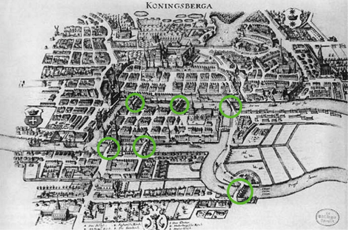
Figure 4.1 Map by Merian‐Erben (1652) showing the city of Königsberg.
Source: Merian‐Erben / wikimedia commons / Public Domain Mark 1.0.
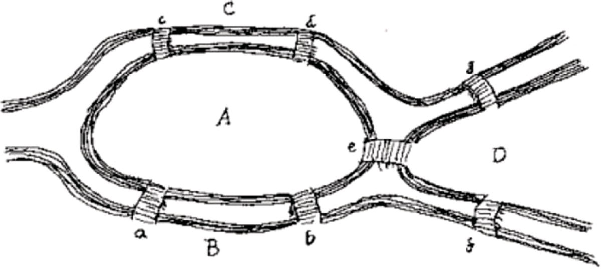
Figure 4.2 Euler's drawing of the Königsberg bridges.
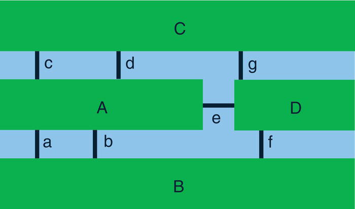
Figure 4.3 Königsberg bridges as links and distinct mainlands as nodes.
Euler indicated that the only important information in this particular problem was the sequence of the bridges to be crossed. Then, it was possible to discard any other information except the number of bridges connecting two land masses. Consequently, the number of bridges was more important than the bridges location. Euler drew the following diagram to formulate the problem. It contains the islands, the mainland, and the bridges. This diagram contains two islands denoted as C and B, and two land masses, denoted as A and D. The seven bridges are denoted as a, b, c, d, e, f, and g. Figure 4.2 shows Euler's drawing of the Königsberg bridges problem.
Extrapolating this problem to build a graph, each land mass is a node (C and D), as well as each island (A and D), and each bridge is a link (a, b, c, d, e, f, and g). Figure 4.3 describes the structure in terms of nodes and links.
As Euler noticed, in this type of problem, only the connections constitute relevant information. The graph can be represented in different shapes without changing the graph itself. The existence or absence of a link between a pair of nodes represents everything in terms of the network. Figure 4.4 describes the problem in terms of a graph, with nodes and links within a connected structure.
The links constitute the only relevant information in this problem and raise a very important concept in network analysis and network optimization. Even when calculating individual network metrics for the nodes, the links are what is considered to compute these centralities. For example, the degree centrality of a node is the number of connections incident to it, or the number of links the node has. No individual information or characteristic of the node itself is relevant, just the links, or particularly here, the number of links in this node. The related nodes are defined by the links between that node and the nodes connected to it. Then, that node's centrality degree for instance is computed by counting the number of links incident to it. Most of the network centralities rely exclusively on the links and the links’ characteristics or attributes, such as the links’ weight between the nodes. Several network optimization algorithms also rely only on the links and its attributes. Finally, as we saw before, most of the methods to detect subgraphs also rely on the links and the links’ characteristics.
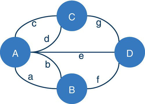
Figure 4.4 Königsberg bridges problem as nodes and links.
Let's go back to the seven bridges problem. Euler observed that whenever a walker gets a bridge (link) and reaches a land mass (node) by a bridge, they leave the node by a link, in a graph perspective. In practical terms, during any walk through the city, the number of times a walker enters a bridge is equal to the number of times they leave a bridge.
In a mathematical formalism, Euler said that the existence of a path in a particular graph depends on the nodes' degrees. We already saw that the degree of a node is the number of links it has, regardless of whether or not the link is arriving to or departing from it. Then, the important information in this problem is the number of links incident to each node. Based on Euler's observation, a necessary condition for a walk through the city is that the graph should be connected and have zero or two nodes with odd degrees. This graph has all four nodes with odd degrees (three connections each). This concept was formulated as the Euler Path. First, the graph must be traversable, which means, we can trace over the links of a graph exactly once without lifting our pencil. Second, the graph needs to have only 2 odd nodes. Third, the walk will start and stop on different odd nodes.
An alternative formulation for the seven bridges problem is to discover a path by which all bridges are crossed and the starting and ending points are the same. This path is known as the Euler Circuit, and this walk exists only if the graph is connected (traversed) and there are no nodes with degrees having odd values.
At the end, Euler proved that the number of the bridges should be even. If a walker wants to cross each bridge once and travel to each part of the city, the number of bridges should be six instead of seven. The solution views each bridge as an endpoint, a link in mathematical terms, connecting the nodes, or the mainland in the city. Euler noticed that only an even number of links produced the correct result of being able to reach every part of the city’s mainland without crossing a bridge twice. He mathematically proved it was impossible to cross all seven bridges only once and visit every part of the city.
The Euler solution to this problem evolved to a mathematical field of study called topology. In computing, topology is useful to understand networks, the flow of information throughout the network, or paths within a system. The Seven Bridges of Königsberg is similar to another common problem in network optimization called Traveling Salesman Problem (TSP), where we try to find the most efficient route given a set of places to visit, with some restrictions, just like in the seven bridges problem. We will see the TSP in more detail later in this chapter. For now, it is good to know that we experience the TSP in our daily lives, when we use our cars, we get on a train, bus or even airplanes. We need to figure out the most efficient way to travel from one place to another, particularly when we need to cover multiple destinations. We also face the TSP when we receive our purchases delivered by online vendors. They are definitely the ones that need to account for the TSP in order to find the most efficient way to deliver all the goods purchased by multiple customers located at different addresses. The most efficient way may represent the minimum time or eventually the delivery’s minimum cost.
This type of problem is perfect for computing because computers are faster and more efficient than humans in calculating things. But before asking computers to do all these calculations, we need Euler and other authors to formulate the problems and define solutions based on mathematical formulas. Then we can create programs to do all the math for us, based on those formulas to run on computers.
In this chapter we will cover some of those algorithms we experience or face in our daily lives, even if we don't really notice them. Algorithms like the TSP, Shortest Path, Minimum Cost Network Flow, Minimum Cut, Minimum Spanning Tree, and Vehicle Routing Problem (VRP) are just some of them.
4.1.2 Network Optimization in SAS Viya
Proc OptNetwork provides several network optimization algorithms that can augment more generic mathematical optimization approaches. Many practical applications of network optimization depend on an underlying network topology. For example, retailers facing the problem of shipping goods from warehouses to stores in a distribution network to satisfy demand at minimum cost. Commuters choosing routes in a road network to travel from home to work in the shortest time. Retailers searching for optimal routes to reach out to multiple destinations at the minimal time. Drivers looking for specific vehicle routes to minimize the distance traveled based on certain conditions. Industries defining teams to produce products at the maximum profitability or establishing quantities of production to minimize the cost. There are endless examples where network optimization can be applied to solve real‐world problems, in virtually any industry.
Networks can be explicit and implicit in different scenarios. Networks are often built based on relationships that occur within those scenarios. For instance, relationships between researchers who coauthor articles, or actors who appear in the same movie, words or topics that occur in the same document, items that appear together in a shopping basket, messages exchanged by subscribers, money wired by customers, these are all explicit relations that create networks. Terrorism suspects who travel together or are seen in the same location, infected people been at the same location at the same time, these are all implicit relations that can also create networks. In both types of relationship, the entities involved in the relations (customers, authors, terrorists) are the nodes within the network. The interactions between them (money, message, flight) are the links within the network. The strength, value, importance, or frequency of these interactions are modeled as weights on the corresponding links of the network. These weights are crucial when running most of the network optimization algorithms.
Most of the network problems described here can actually be solved by using traditional optimization approaches, or general methods, like linear programming or mixed integer linear programming. Nevertheless, proc OptNetwork provides a set of optimization algorithms specifically tailored to network problems. These methods implemented in proc OptNetwork require less coding by the users and offer superior computational performance.
Proc OptNetwork makes no assumption about the context or application considered when building the network. The procedure provides a set of network analysis and network optimization algorithms that take an abstract graph or network as input. The procedure’s outcomes help users to better understand the network structure and guide them in solving specific network optimization problems. Depending on the application or business problem, this type of network analysis can stand on its own and provide independent value or final solution to the problem. In some other business scenarios, the network analysis can provide additional input for subsequent work in optimization, or even in other forms of analytics, like supervised and unsupervised machine learning models.
Similar to what we see in Chapter 3 for proc Network, proc OptNetwork requires a graph G = (N, L), where N is defined as a set of nodes and L is defined as a set of links. A node is an abstract representation of some entity or object within the network, and a link defines the relationship or connection between two entities or objects. Often, the terms node and vertex are interchangeable in describing an entity. Analogously, the term link is interchangeable with the terms edge or arc in describing a connection, interaction, or relationship between two nodes. Finally, the terms graph and network are also interchangeable.
4.2 Clique
A clique of a graph is a subgraph that is a complete graph. In a complete graph, every node within the graph is connected to every other node. A clique is then a subgraph within a graph where every node in the clique is connected to each and every other node within the same clique. In large graphs, it is easy to find cliques within the network, and sometimes cliques within cliques. Then, there is an important concept known as the maximal clique. A maximal clique is a clique that is not a subset of the nodes of any larger clique. That is, it is a set C of nodes such that every pair of nodes in C is connected by a link and every node not in C is missing a link to at least one node in C. The number of maximal cliques in a graph can be quite large and can grow exponentially with every node that is added to the network.
Cliques in network analysis and network optimization have multiple applications. Industries like bioinformatics, social sciences, electrical engineering, and chemistry are good candidates for problem solving by using the concepts of cliques. The analysis of transportation systems and traffic routes can also benefit from the concept of cliques. Even analytical models in banking, insurance and money laundering can use outcomes provided by clique analysis.
Proc optnetwork finds the maximal cliques of a graph by using the CLIQUE statement. The clique algorithm works only with undirected graphs (with no self‐links). Clique can be seen as a sequence of nodes where, from each of the nodes within the graph, there is a link to the next node in that sequence.
The results of the clique algorithm are written to the output data table that is specified in the OUT= option. The output lists each node of each clique along with the variable clique to identify the clique to which it belongs. The clique identifiers are numbered sequentially, starting from the value of the INDEXOFFSET= option in the proc optnetwork statement. Proc optnetwork can find multiple cliques in the same run. Then, a particular node can appear multiple times in the output dataset if it belongs to multiple cliques.
The INDEXOFFSET= option in proc optnetwork specifies the index offset for identifiers in the log and results output tables. For example, if there are three cliques within the network, the clique enumeration algorithm labels the cliques as 1, 2, and 3. If INDEXOFFSET= 4, the clique enumeration algorithm labels the cliques as 4, 5, and 6. The value assigned to the INDEXOFFSET= option must be an integer greater than or equal to 0. By default, INDEXOFFSET= option is 1.
Proc optnetwork can compute all maximal cliques within the network. For very large graphs, proc optnetwork may not scale well in enumerating all maximal cliques.
If we simply want to count the cliques, we just need to suppress the output option and proc optnetwork will not write the results. If we suppress all options, just invoking the clique algorithm, proc optnetwork will return just the first clique.
In proc optnetwork, the CLIQUE statement invokes the algorithm that finds the maximal cliques in the input graph.
There are many options to be set when running proc optnetwork to find the maximal cliques within a graph.
The MAXCLIQUES= option specifies the maximum number of cliques for clique enumeration to return. We can specify a number (which can be any 32‐bit integer greater than or equal to 1) or ALL (which represents the maximum that can be represented by a 32‐bit integer). By default, MAXCLIQUES = 1.
The MAXLINKWEIGHT= option specifies the maximum sum of link weights in a clique. Any clique in which the sum of the link weights is greater than the number specified is removed from the results. This option can be used to discard a sequence of very strong relations between the links, and then, as a result, to reduce the number of possible maximal cliques within the network. The default value for this option is the largest number that can be represented by a double. When the default is used, no cliques are removed from the final results, or all possible maximal cliques are output.
The MINLINKWEIGHT= option specifies the minimum sum of link weights in a clique. Any clique in which the sum of the link weights is less than the number specified in the option is removed from the results. This option can be used to discard a sequence of very weak relations between the links, and then, as a result, to reduce the number of possible maximal cliques within the network. The default value for this option is the largest negative number that can be represented by a double. When the default is used, no cliques are removed from the final results.
The MAXNODEWEIGHT= option specifies the maximum sum of node weights in a clique. Any clique in which the sum of the node weights is greater than the number specified is removed from the results. Analogous to the link weights, this option can be used to discard a sequence of relations between very strong nodes, and then, as a result, to reduce the number of possible maximal cliques within the network. The default is the largest number that can be represented by a double. When the default is used, no cliques are removed from the final results.
Similarly, the MINNODEWEIGHT= option specifies the minimum sum of node weights in a clique. Any clique in which the sum of the node weight is less than the number specified in the option is removed from the results. Again, analogous to the link weights, this option can be used to discard a sequence of relations between weak nodes, and then, as a result, to reduce the number of possible maximal cliques within the network. The default value for this option is the largest negative number that can be represented by a double. When the default value is used, no cliques are removed from the final results.
There is a useful option in proc optnetwork when computing cliques. The MAXSIZE= option specifies the maximum number of nodes in a clique. Any clique in which the size is greater than the number specified is removed from the results. This option is useful in well‐connected networks, where the maximal cliques can be quite large. The default is the largest number that can be represented by a 32‐bit integer. When the default is used, no cliques are removed from the results. For example, if we are trying to find triangles, a common concept in fraud detection or money laundering, we can invoke the clique enumeration algorithm in proc optnetwork to limit the number of nodes in each clique to 3. Then proc optnetwork finds just cliques with a maximum of 3 nodes. We may find cliques with just 2 nodes though. Another option can be used to specifically determine cliques with 3 nodes.
The MINSIZE= option complements the MAXSIZE= option in searching cliques with specific sizes. This option specifies the minimum number of nodes in a clique. Any clique in which the size is less than the number specified in the option is removed from the results. By default, MINSIZE = 1 and no cliques are removed from the results. This option can complete the search for specific size cliques in the fraud detection and money laundering example. If we are looking for cliques with exactly 3 nodes, we can specify MINSIZE = 3 and MAXSIZE = 3. Then proc optnetwork finds only triangles within the network.
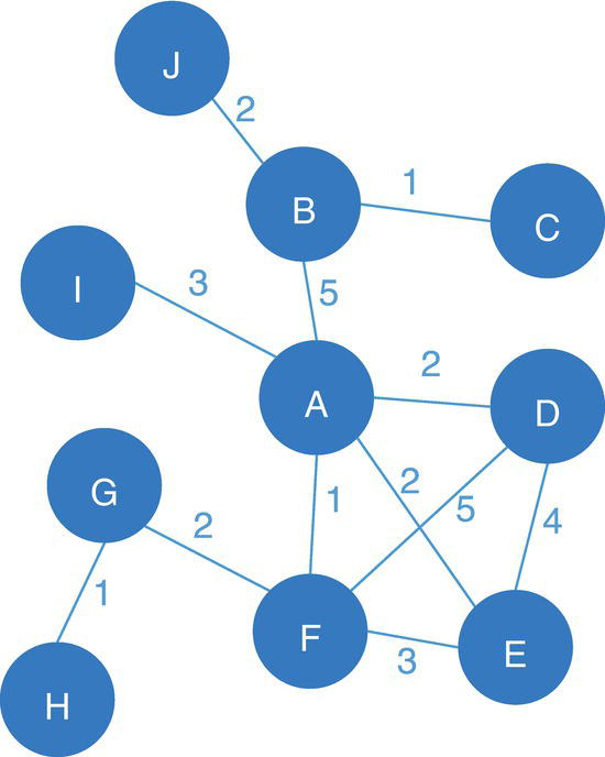
Figure 4.5 Undirected graph with weighted links.
As we notice, clique enumeration can be exhaustive, particularly in large graphs. Proc optnetwork allows us to limit the time of running when invoking the network optimization algorithms. The MAXTIME= option specifies the maximum amount of time to spend finding all maximal cliques within the network. The type of time is determined by the value of the TIMETYPE= option. If TIMETYPE=CPU, the restriction of time is applied per processing machine. If TIMETYPE=REAL, the number specified in the MAXTIME= option defines the units of real‐time. By default, the time type is real. The default value for the MAXTIME= option is the largest number that can be represented by a double.
The last option is where to output the results. The OUT= option specifies the output data table contains all maximal cliques found by proc optnetwork. The output data table must be a CAS‐libref.data‐table, where CAS‐libref refers to the caslib, and data‐table specifies the name of the output data table.
4.2.1 Finding Cliques
Let's consider the undirected graph with weighted links presented in Figure 4.5. This graph is similar to the ones we used to demonstrate the network centralities, except for the additional link between D and F with weight of 5.
The following code describes how to create the new links dataset and search for the maximal cliques within the undirected graph.
data mycas.links;input from $ to $ weight @@;datalines;J B 2 B C 1 B A 5 I A 3 D A 2 A E 2 A F 1 G F 2 G H 1 E F 3 D E 4 D F 5;run;proc optnetworkdirection = undirectedlinks = mycas.links;cliquemaxcliques = allout = mycas.outclique;run;
A summary result is created for each execution of proc optnetwork. Figure 4.6 shows the results for the clique algorithm.
As a result, proc optnetwork finds seven cliques, including all pairs of nodes (J‐B, B‐C, B‐A, I‐A, G‐F, and G‐H) plus the clique comprising 4 nodes (A‐D‐F‐E). We can see this list checking the output dataset.
Proc optnetwork generates the output dataset OUTCLIQUE presented in Figure 4.7 containing all maximal cliques found. The dataset shows the identification for each clique and the nodes belonging to them.
We can set the minimum and the maximum size for the cliques searched by proc optnetwork. This constraint forces proc optnetwork to produce less cliques within the network as a final result. The following code specifies that all cliques found by proc optnetwork must have at least 3 nodes and the maximum of 10 nodes.

Figure 4.6 Summary results for clique enumeration using proc optnetwork.
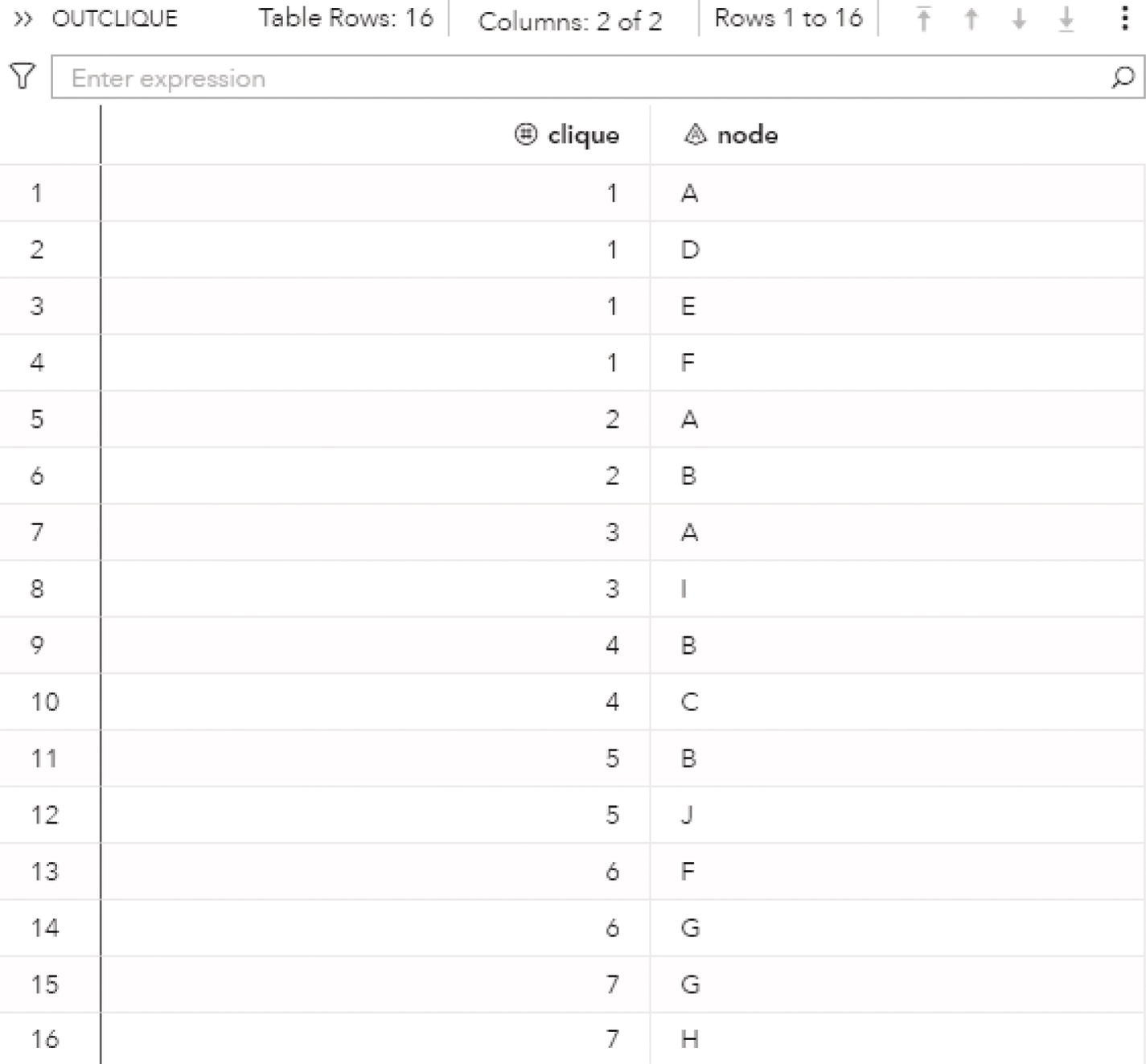
Figure 4.7 Output dataset for the cliques.
proc optnetworkdirection = undirectedlinks = mycas.links;cliquemaxcliques = allminsize = 3maxsize = 10out = mycas.outclique;run;
With the constraints for the minimum and maximum number of nodes within the clique, proc optnetwork finds only 1 clique. Figure 4.8 shows the summary results for the clique algorithm.
The output dataset OUTCLIQUE presented in Figure 4.9 shows the nodes assigned to the single clique. The single clique founds has 4 nodes, A, D, E, and F.
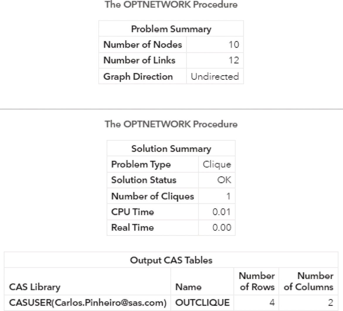
Figure 4.8 Output results for proc optnetwork searching for cliques.
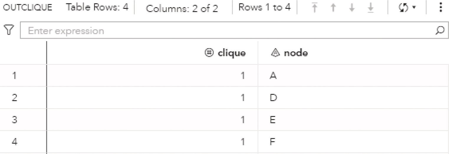
Figure 4.9 Output dataset with the nodes within the single clique.
Figure 4.10 highlights the single clique based on the constraints for minimum and maximum number of nodes.
Finally, depending on the constraints specified, proc optnetwork may return no results. For instance, if we increase the minimum number of nodes in the clique to 5, proc optnetwork will not find any clique within the network.
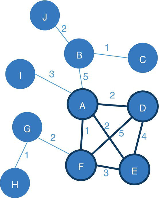
Figure 4.10 Single clique within the network based on a set of constraints.
proc optnetworkdirection = undirectedlinks = casuser.links;cliquemaxcliques = allminsize = 5out = casuser.outclique;run;
The summary results presented in Figure 4.11 show that there is no clique found within the network based on the constraints defined.

Figure 4.11 No cliques found with a minimum of 5 nodes.
As a final note on the clique enumeration, large graphs can produce a huge number of cliques, and make the computational process take too long to run or even be unfeasible. A good practice in searching for cliques in large networks is to define constraints to limit the minimum and maximum sizes for the cliques, the minimum and maximum link weights to form the cliques, the minimum and maximum node weights to compose the cliques, the maximum time to run the algorithm, and finally, the maximum number of cliques returned for the clique enumeration.
4.3 Cycle
A sequence of links where the destination node of each link is the origin node of the next link is known as a path. Cycle is an elementary path in a graph where the starting node is also the ending node. No node within the path can appear more than once in the sequence. For example, a sequence of connections such as A → B → C → D → A.
Proc optnetwork searches for elementary cycles in a graph. A graph can comprise multiple cycles. Proc optnetwork searches and counts all cycles within that graph.
Cycles in network analysis and network optimization have several business applications. Social sciences, computer networks, and logistics are common candidates for cycle enumeration used when solving real‐world problems. Like clique enumeration, cycles can also be used in transportation systems and as part of a broader set of analytical models to find anomaly transactions in banking, insurance, and mostly money laundering.
The results of the cycle enumeration algorithm are written to the output data tables that are specified in options. Proc optnetwork can provide one output for the nodes and one for the links. We can also simply define the OUT= option to produce a single data table as the result of the cycle enumeration. This output lists each node of each cycle along with the variable to identify to which cycle the node belongs and the order of that node in the cycle. Analogous to the clique enumeration algorithm, the cycle identifiers are numbered sequentially, starting from the value of the INDEXOFFSET= option in the proc optnetwork statement. Proc optnetwork can find multiple cycles within the same network at the same run. Therefore, a particular node can appear multiple times in the output dataset if it belongs to multiple cycles. The INDEXOFFSET= option is explained in the clique enumeration algorithm.
Proc optnetwork can search and count all cycles within the network. For very large graphs, proc optnetwork may not scale well in enumerating all cycles existing in the network. We can always define constraints to limit the number of cycles that will be searched and counted along the process.
In proc optnetwork, the CYCLE statement invokes the algorithm that finds the cycles in the input graph.
There are many options to define how proc optnetwork runs when counting cycles within a graph. If we suppress the output options, proc optnetwork simply counts the number of elementary cycles within the graph.
We can simply specify the option OUT= to have a single output data table as the result of the cycle algorithm, or we can specify the options OUTCYCLESNODES= to report the nodes in which cycle, and its order, similarly to the OUT= option, and the option OUTCYCLESLINKS= to report the links in which cycle, and its order.
The cycle enumeration is primarily tailored to directed graphs. It makes more sense when a sequence of nodes connected to each other creates a path where the origin node is the final node too. However, cycles can also be found in undirected graphs. In this case, each link represents two directed links, in both directions. For example, a link A − B represents two links in both directions, A → B and B → A .This can generate a substantial number of cycles in the final report. For this reason, trivial cycles like A → B → A and duplicate cycles found by traversing a cycle in both directions like A → B → C → A and A → C → B → A are filtered out from the results.
Proc optnetwork uses two different algorithms to enumerate cycles. If the MAXLENGTH= option is greater than 20, the algorithm used is the backtracking (ALGORITHM=BACKTRACK). This can properly scale to large graphs that contain few cycles. However, some graphs can have a large number of cycles, so the algorithm might not scale well. If the MAXLENGTH= option is less than or equal to 20, then the algorithm used is the Build (ALGORITHM=BUILD). This algorithm is usually faster than the backtracking algorithm when the length of the cycles is sufficiently restricted. Those are the default options. Users can always change the default setting by using the option ALGORITHM=BACKTRACK|BUILD.
When searching and counting all cycles in a graph, the output table can become very large. The option MAXCYCLES=ALL requests proc optnetwork to count all cycles in a graph. A good practice before outputting the results is to simply verify the number of cycles within the network by suppressing the OUT= option. If the number of cycles is not too large, the output data table can be used subsequently to report all the cycles.
The option OUTCYCLESNODES= (or OUT=) creates the output table containing the enumerated cycles as a sequence of nodes. This table contains the following columns:
- cycle: the cycle identifier
- order: the order of the node in the cycle
- node: the node label
The option OUTCYCLESLINKS= creates the output table containing the enumerated cycles as a sequence of links. This table contains the following columns:
- cycle: the cycle identifier
- order: the order of the link in the cycle
- from: the from (origin) node label
- to: the to (destination) node label
The MAXCYCLES= option specifies the maximum number of cycles that proc optnetwork returns based on the cycle enumeration algorithm. The number specified ranges from 1 to the greatest number defined by a 32‐bit integer. The option ALL returns all cycles existing in the network, limit to a maximum number that can be represented by a 32‐bit integer. By default, MAXCYCLES = 1.
The option MAXLENGTH= specifies the maximum number of links in a cycle. Any cycle containing more links than the number specified in the option is removed from the results. The default is the largest number that can be represented by a 32‐bit integer. When the default is used, no cycles are removed from the results.
The MINLENGTH= option specifies the minimum number of links in a cycle. Any cycle containing less links than the number specified in the option is removed from the results. By default, MINLENGTH = 1 and no cycles are removed from the results.
The option MAXLINKWEIGHT= specifies the maximum sum of link weights in a cycle. Any cycle with the sum of all its link weights greater than the number specified in the option is removed from the results. The default is the largest number that can be represented by a double. When the default is used, no cycles are removed from the results.
The option MINLINKWEIGHT= works similarly. It specifies the minimum sum of link weights in a cycle. Any cycle with the sum of all link weights less than the number specified in the option is removed from the results. The default is the largest negative number that can be represented by a double. When the default is used, no cycles are removed from the results.
The option MAXNODEWEIGHT= specifies the maximum sum of node weights in a cycle. Any cycle with the sum of all node weights greater than the number specified in the option is removed from the results. The default is the largest number that can be represented by a double. When the default is used, no cycles are removed from the results.
The MINNODEWEIGHT= option specifies the minimum sum of node weights in a cycle. Any cycle with the sum of all node weights less than the number specified in the option is removed from the results. The default is the largest negative number that can be represented by a double. When the default is used, no cycles are removed from the results.
Similar to the clique enumeration, a graph may contain a great number of cycles. The process can be exhaustive and require a long computing time. To avoid proc optnetwork from running for long periods, we can limit the amount of time the procedure will run to search all cycles within the network. The option MAXTIME= specifies the maximum amount of time to spend finding cycles. The type of time is CPU time or real‐time. This is determined by the option TIMETYPE= in the proc optnetwork. The default value is the largest number that can be represented by a double.
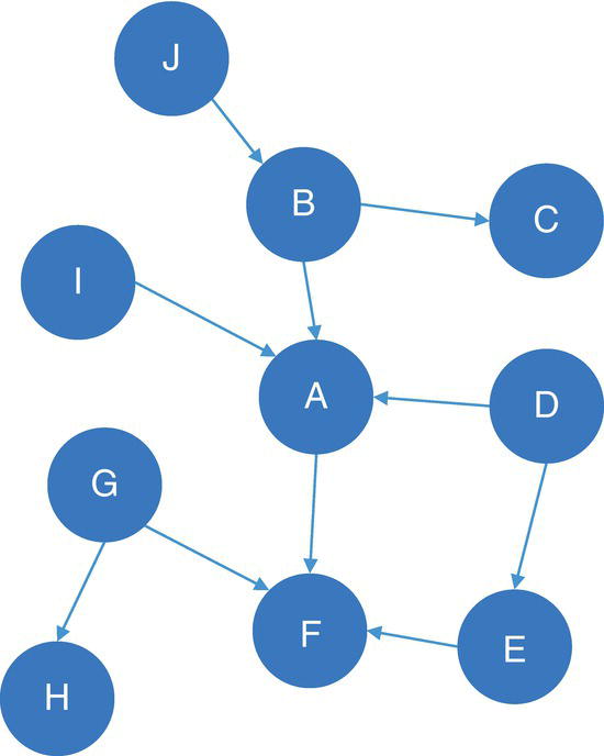
Figure 4.12 Directed graph with unweighted links.
4.3.1 Finding Cycles
Let’s consider the directed graph with unweighted links presented in Figure 4.12. This graph is similar to the previous graph except by one missing link between A and E.
The following code describes how to create the new links dataset and then search for the existing cycles within the directed graph.
data mycas.links;input from $ to $ @@;datalines;J B B C B A I A A D F A G F G H E F D E;run;proc optnetworkdirection = directedlinks = mycas.links;cyclemaxcycles = alloutcyclesnodes = mycas.outcyclenodesoutcycleslinks = mycas.outcyclelinks;run;
Figure 4.13 shows the summary result created by proc optnetwork after the execution.
As a result, proc optnetwork finds one single cycle, formed by A → D → E → F → A.
The output dataset OUTCYCLENODE presented in Figure 4.14 contains the cycle found as a sequence of nodes. The dataset contains the identification for the cycle, the nodes within that cycle, and their order within the cycle.
The output dataset OUTCYCLELINK presented in Figure 4.15 contains the cycle found as a sequence of links. The dataset contains the identification for the cycle, the order of the link, the from (origin) node, and the to (destination) node
Analogously to the clique enumeration, the cycle enumeration can produce a high number of cycles, particularly in large networks, making the computational process exhaustive and long. A good practice in searching for cycles, especially in large graphs, is to define constraints to limit the possible number of cycles to be found and reported in the output datasets, which includes the size of the cycle, the link weights, the node weights, the time to run, and of course, the maximum number of cycles to be returned.

Figure 4.13 Summary results for cycle enumeration using proc optnetwork.
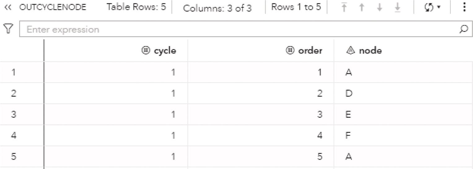
Figure 4.14 Output dataset containing the nodes within the cycle.
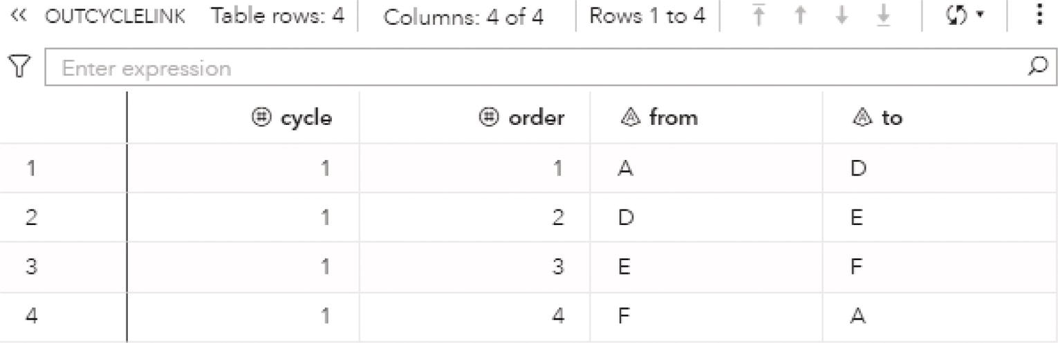
Figure 4.15 Output dataset containing the cycles.
Figure 4.16 highlights the single cycle found in the input graph.
4.4 Linear Assignment
The linear assignment problem is a fundamental problem in combinatorial optimization that involves assigning workers to tasks at minimal costs. In graph theoretic terms, linear assignment is equivalent to finding the minimum link weights matching in a weighted bipartite directed graph. In a bipartite graph, the nodes can be divided into two disjointed sets W (workers) and T (tasks). Links connect nodes between both sets W and T, but not nodes within each set W or T. That means, the sets of nodes W and T are independent. There are no connections inside sets W and T, just connections between nodes from W and T. The concept of assigning workers to tasks can be generalized to the assigning of any abstract object from one group to some abstract object to another group.
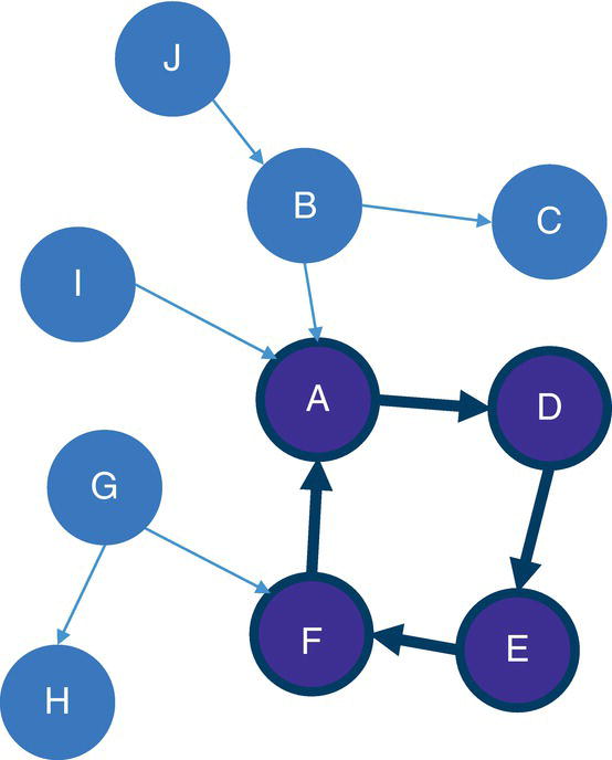
Figure 4.16 Single cycle within the input graph.
The linear assignment problem can be formulated as an integer programming optimization problem. The form of the problem depends on the sizes of the two sets of nodes W and T.
Let's assume that A represent the set of possible assignments between the sets of nodes W and T. In a bipartite graph, these assignments are the links between the nodes, or the workers and the tasks.
First, let's define some rules for the optimization problem, like the decision variables, the objective function, and the constraints for the possible solutions.
The decision variable can be defined as
Otherwise, x w,t = 0.
The objective function can be defined as:
The solution is subjected to some constraints, such as each worker is assigned to one single task, each task is assigned to one single worker, and finally, the cost of the worker doing the task is always positive.
If the number of workers is greater than or equal to the number of tasks (∣W ∣ ≥ ∣ T∣), then the optimization problem can be solved as follows:
where c a is the cost of the assignment a associated with x a , which is the worker w doing the task t. The ![]() represents the set of outgoing links that are connected from node w (the workers) and
represents the set of outgoing links that are connected from node w (the workers) and ![]() represents the set of incoming links that are connected to node j (the tasks).
represents the set of incoming links that are connected to node j (the tasks).
In the case of the number of workers being strictly greater than the number of tasks (∣W ∣ > ∣ T∣), the model allows for some workers to go unassigned.
If the number of workers is less than the number of tasks (∣W ∣ < ∣ T∣), then the optimization problem can be solved as follows:
In this case, the model allows for some tasks to go unassigned.
In proc optnetwork, the LINEARASSIGNMENT statement invokes the algorithm that solves the minimal‐cost linear problem. This algorithm is based on the augmentation of shortest paths. It can be applied only to bipartite graphs. For the matching problem, we first define the input graph as a directed network by specifying the DIRECTION= option as directed. Then we use the LINK= option to define how the links dataset will determine the problem. The workers are set in the FROM= option. The tasks are set in the TO= option. Finally, the cost to perform a task by a worker is set in the WEIGHT= option. Internally, the graph is treated as a bipartite graph where the from nodes define one set, and the to nodes define the other set.
There are few options for the linear assignment algorithm in proc optnetwork.
The resulting assignment is reported in the output data table specified in the OUT= option. The resulting matching table keeps the same from, to, and weight column names. The output table is a two‐level name, including the caslib name and the output table name.
The option MAXTIME= specifies the maximum amount of time that the linear assignment algorithm will spend to find the solution. The type of time can be either CPU time or rea‐ time, and it is determined by the value of the TIMETYPE= option. The default is the largest number that can be represented by a double.
4.4.1 Finding the Minimum Weight Matching in a Worker‐Task Problem
Let's consider the bipartite graph containing the relationship between workers and tasks presented in Figure 4.17. Each relation describes the cost to produce each part of a chair by each one of the workers.
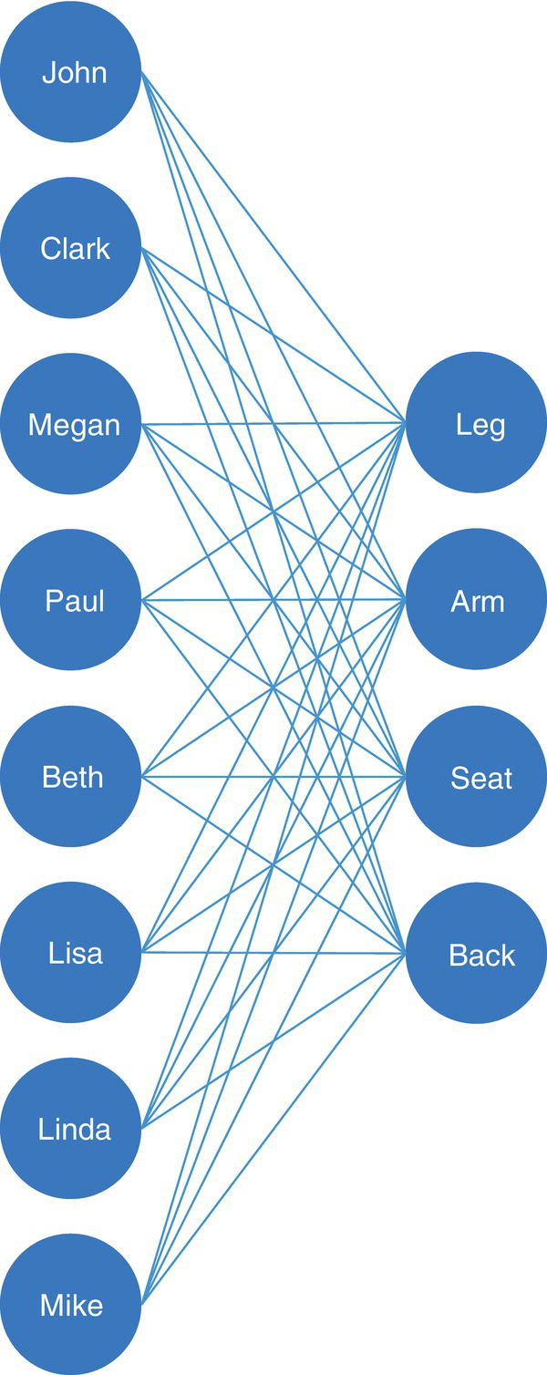
Figure 4.17 Bipartite graph with relations between workers and tasks.
The following code describes how to create the bipartite graph containing the cost of each worker to produce each one of the pieces of a chair. We can directly create a table with all the workers repeating as lines for their costs to build each piece of a chair, or we can create a matrix containing workers by pieces containing the respective costs. Let's see the second approach, which seems more elegant.
data mycas.chairs;input employee $ leg arm seat back;datalines;John 14 18 23 27Clark 12 14 19 22Megan 15 17 28 25Paul 21 25 32 19Beth 16 20 22 28Lisa 13 21 20 32Linda 15 19 25 29Mike 15 16 24 26;run;
This first step creates the matrix with 8 lines (workers) and 4 columns (pieces of a chair). Figure 4.18 shows the table representing that matrix.
The second step transposes the matrix into a table, repeating the workers based on their costs to produce each piece of the chair. The result is a table with 32 lines (8 workers repeated 4 times – for each piece of the chair) and 3 columns (the worker, the piece of the chair, and the respective cost). This is the table we need to pass as a parameter to proc optnetwork in order to search for the minimum weight or cost to produce the chairs.
data mycas.chairslinks(keep=employee part cost);set mycas.chairs;length part $ 4;array a[4] leg arm seat back;do i = 1 to dim(a);part = vname(a[i]);cost = a[i];output;end;run;
This second step creates the table presented in Figure 4.19.

Figure 4.18 Matrix workers by pieces of a chair containing the respective costs.
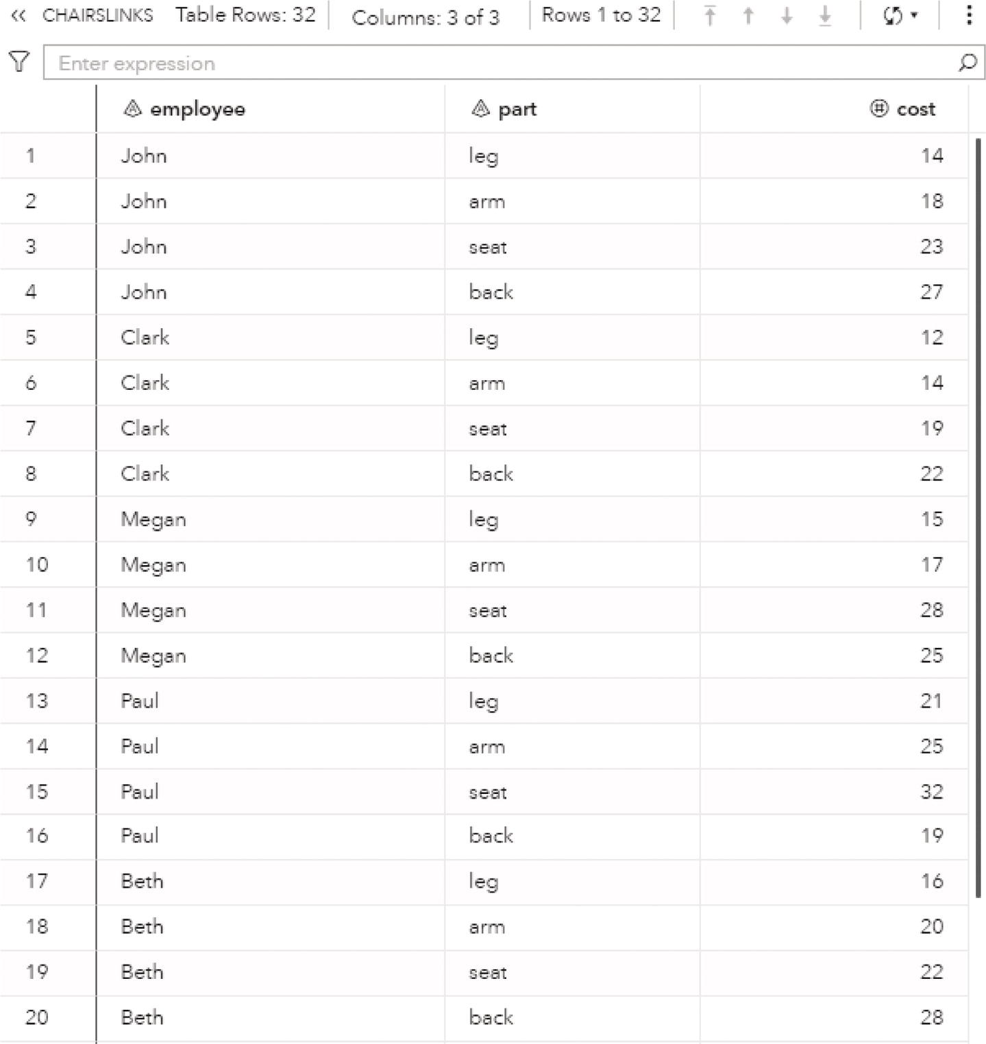
Figure 4.19 Table of workers containing the costs to produce each piece of a chair.
This final table is then passed as a parameter to the proc optnetwork in order to search for the minimum cost to produce chairs. The linear assignment algorithm will search for the combination of workers and pieces of a chair to minimize the cost (the weight).
The following code invokes the linear assignment algorithm in proc optnetwork. Notice that in the linksvar= option the weight receives the cost to produce the piece of a chair by each worker.
proc optnetworkdirection = directedlinks = mycas.chairslinks;linksvarfrom = employeeto = partweight = cost;linearassignmentout = mycas.outlap;run;
Figure 4.20 shows the output for the linear assignment algorithm. It says an optimal solution was found and the objective function (the minimal cost) is 67.
Figure 4.21 shows the optimal combination, which means which worker should produce which part of the chair in order to minimize the cost of production.
As a result, Clark will produce the arm at cost 14, John will produce the leg at cost 14, Lisa will produce the seat at cost 20, and Paul will produce the back at cost 19. The total cost will be 67, and this will be the minimal cost to produce a chair considering all different costs of all workers to produce each chair’s piece. Notice that Clark is the cheapest for leg, arm, and seat. He was selected for arm so others can be picked to minimize the total cost.
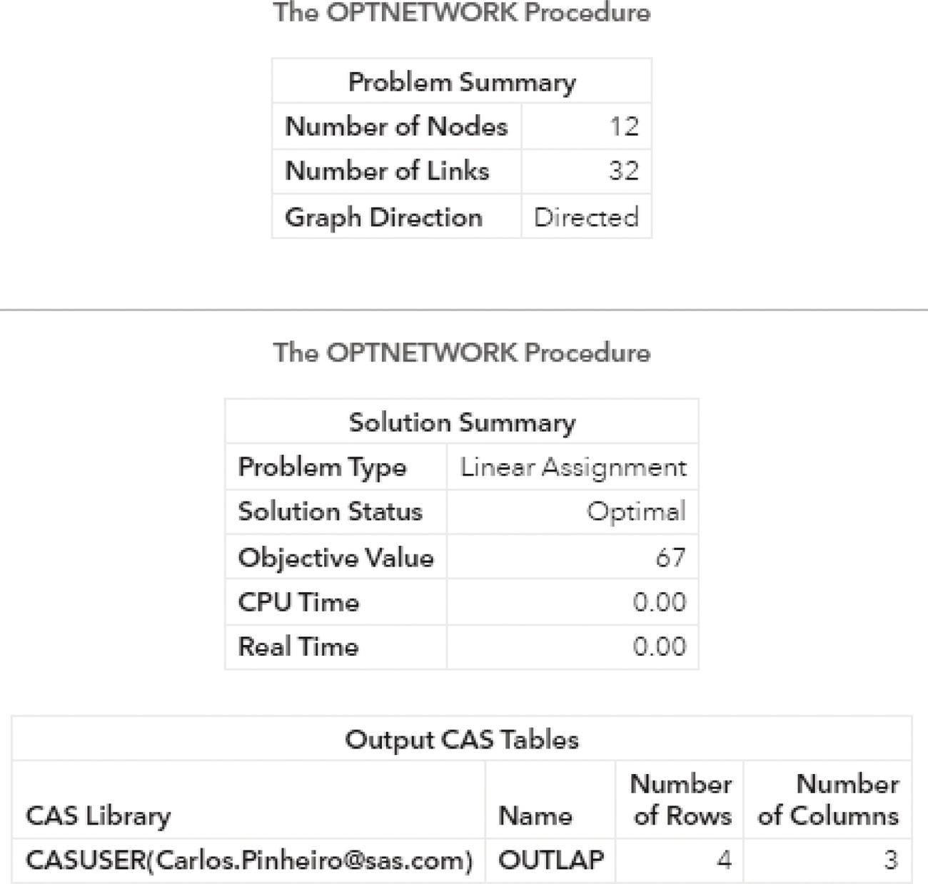
Figure 4.20 Output results by proc optnetwork.
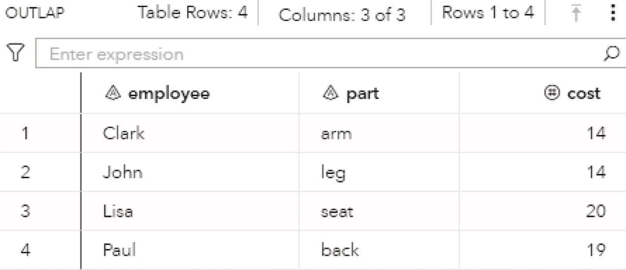
Figure 4.21 Table of selected workers and the costs to produce each piece of a chair.
Figure 4.22 shows how the bipartite graph looks like when the minimal cost is achieved.
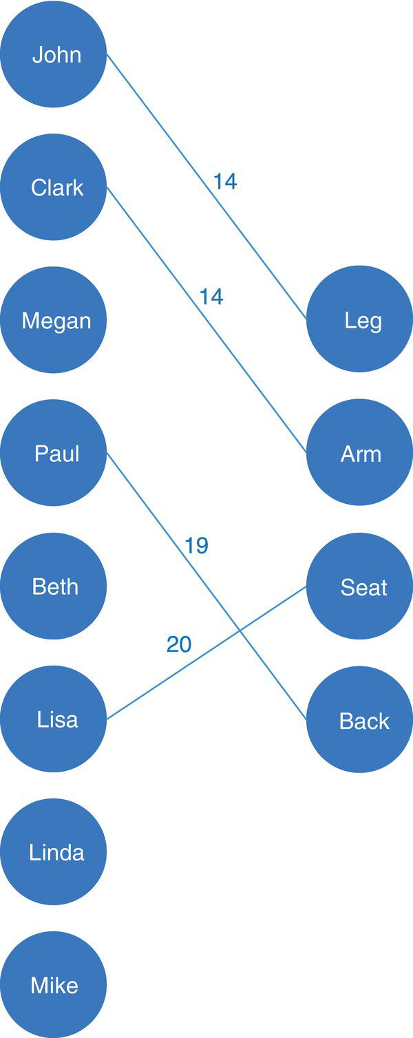
Figure 4.22 Bipartite graph with the optimal match.
Suppose we are trying to maximize the objective function. Instead of minimizing the cost, for instance, we need to maximize the profit. Proc optnetwork doesn't maximize the objective function but if we invert the weights and minimize the objective function, it also works.
Just as an example, let's use the same data, but now producing the inverse weight for the cost. The following code describes this approach:
data mycas.chairslinks(keep=employee part profit invwgt);set mycas.chairs;length part $ 4;array a[4] leg arm seat back;do i=1 to dim(a);part=vname(a[i]);profit=a[i];invwgt=1/a[i];output;end;run;
This code produces the table presented in Figure 4.23, switching cost to profit and producing the inverse of the cost as invwgt.
The following code invokes the linear assignment algorithm in proc optnetwork. Here we are using the option vars= (_all_) in the linksvar statement in order to export all original variables to the result table. With that, we will have the inverse weight, used to minimize the objective function, but also the original weight, here considered as the maximal profit.
proc optnetworkdirection = directedlinks = mycas.chairslinks;linksvarfrom = employeeto = partweight = invwgtvars = (_all_);linearassignmentout = mycas.outlap;run;
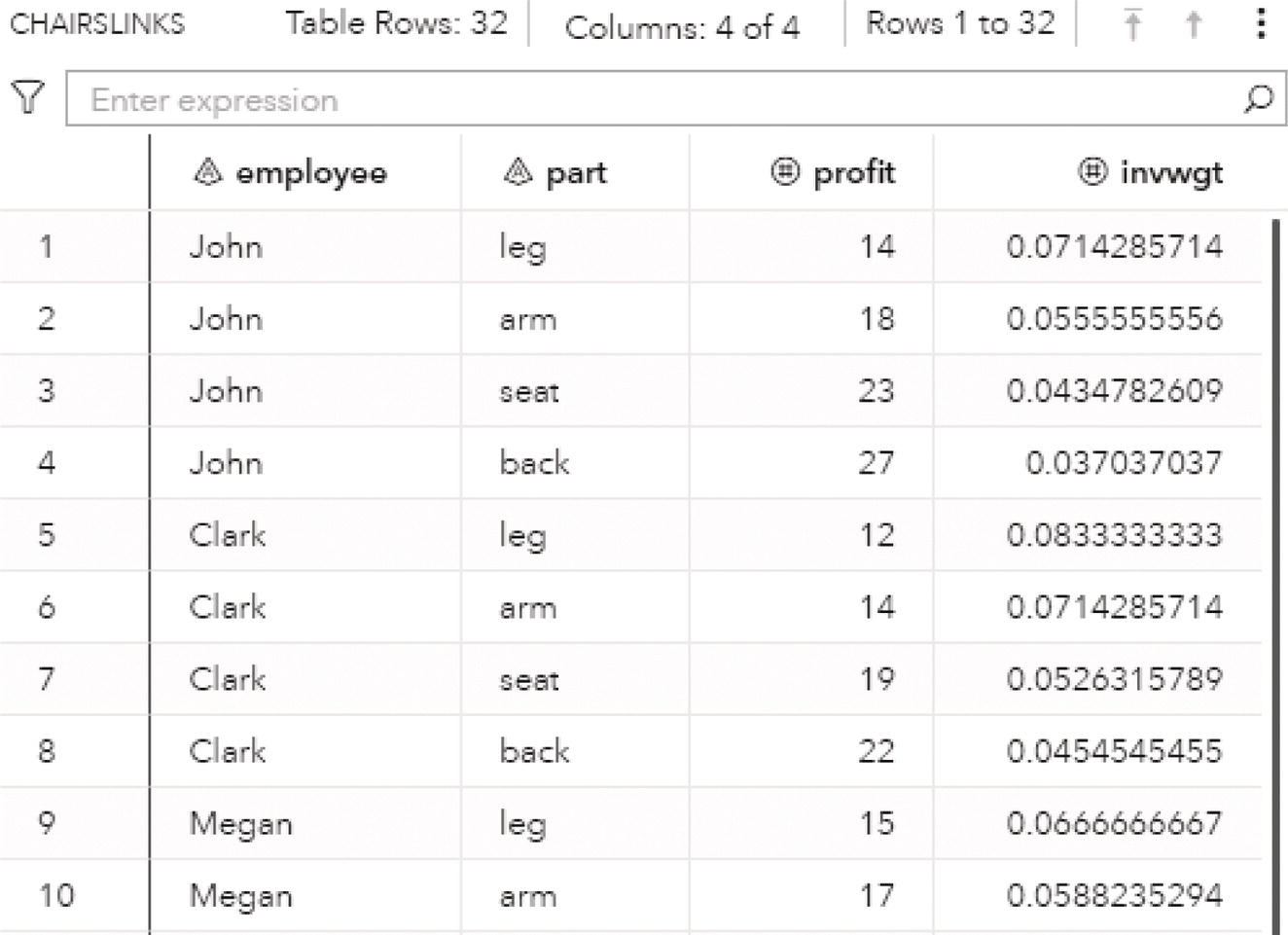
Figure 4.23 Table containing the inverse of the weights.
Proc optnetwork produces the output presented in Figure 4.24. Notice that an optimal solution was found when the objective function was minimized to 0.1645.
Figure 4.25 shows the optimal combination, which means which worker should produce which part of the chair in order to maximize the profit. This scenario doesn't make much sense, but it can illustrate the concept. Translate this example for instance to create a bundle of products and services that maximizes the profit for a telecommunications company.
Notice that the final result produces a total profit (originally cost) as 101. If we think about the cost only, when minimizing the objective function, we found a total cost of 67. Here we minimize the inverse of the cost, which works similarly to maximize the cost. The maximal cost then was 101.
4.5 Minimum‐Cost Network Flow
The minimum‐cost network flow problem is aimed to find the cheapest possible way of sending a certain amount of flow through a network. This problem is useful for a set of real‐life situations involving network with associated costs and flows to be sent through. The minimum‐cost network flow algorithm is commonly applied in telecommunications networks, energy networks, computer networks, and of course, in supply chains.
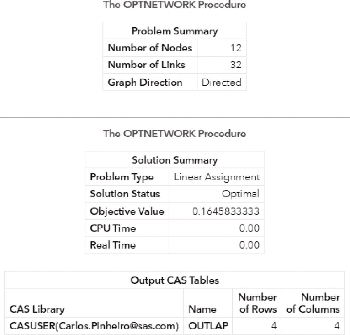
Figure 4.24 Output results produced by proc optnetwork.
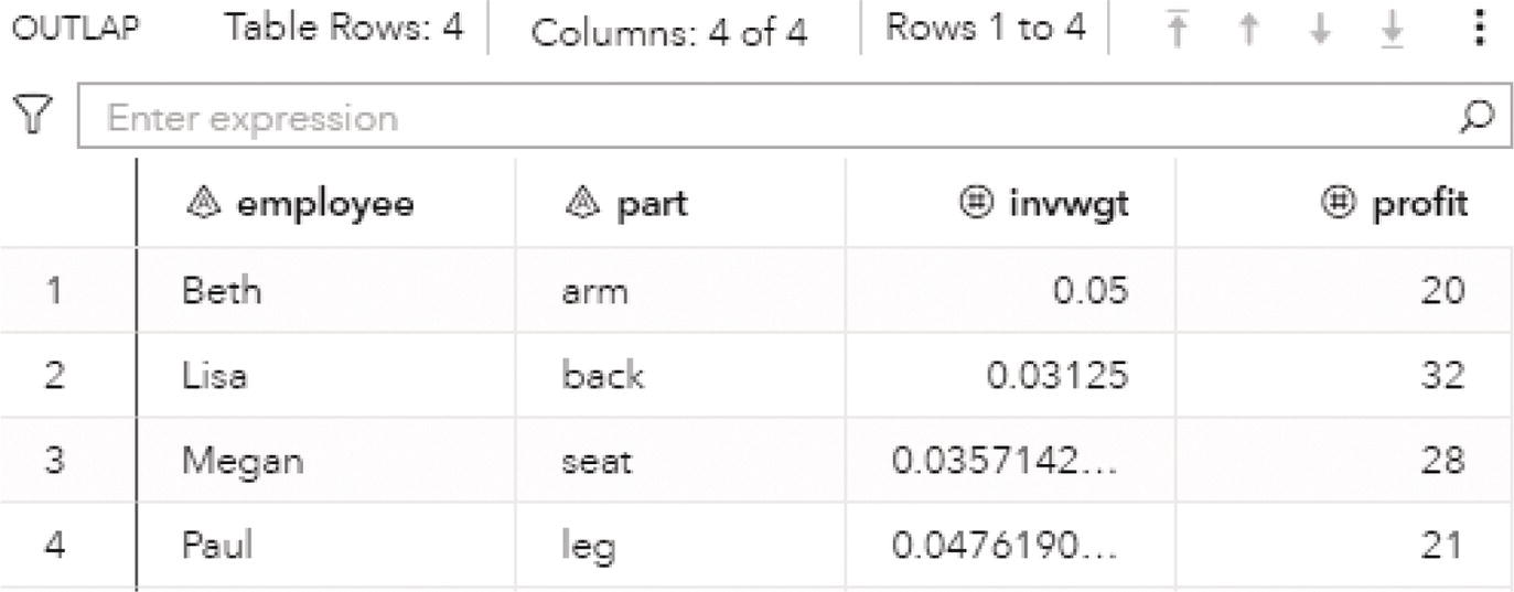
Figure 4.25 Table of selected workers and the costs to produce each piece of a chair.
The minimum‐cost network flow problem is a fundamental problem in network analysis and network optimization that involves sending flow over a network at a minimal cost. Suppose that G = (N, L) is a directed graph, comprising a set of nodes N and a set of links L. For each link (i, j) of L, we can associate a cost per unit of flowing something through the network (goods for example in a supply chain scenario), designated by c ij . The demand or supply at each node i of N is designated as b i , where b i ≥ 0 denotes a supply node, and b i < 0 denotes a demand node. In some cases, when b i = 0, the node is called a transshipment node. These values must be within lower and upper limits when we define the constraints of the business scenario. In this business scenario, we can also define a decision variable x ij . This decision variable represents the number of units flowing through the network, the specific amount of goods sent from node i to node j. As we may have constraints assigned to the nodes, for both demand and supply, defined by the lower and upper limits, we may also have constraints defined to the links. The amount of flow that can be sent across each link can therefore be bounded within [l ij , u ij ]. The lower bound l ij represents the minimum flow that must be sent from node i to node j. The upper bound u ij represents the maximum flow that can be sent from node i to node j and these constraints are optional. That means, we can define or not a minimum amount of goods that need to be sent throughout a link, as well as we may or may not define the maximum amount of flow that can be sent through the link.
The minimum‐cost network flow problem can be modeled as a linear programming problem that minimizes the sum of the cost per unit of flow, that is, the goods that are sent through all the links (i, j) of L, and the lower and upper limits of flows that must or can be sent throughout the links.
The mathematical formulation is represented by the following equations:
Minimize
Subject to
where ![]() represents the set of outgoing links that are connected from node i, and
represents the set of outgoing links that are connected from node i, and ![]() represents the set of incoming links that are connected to node i. The lower and upper limits for the demand or supply for each node was previously defined as
represents the set of incoming links that are connected to node i. The lower and upper limits for the demand or supply for each node was previously defined as ![]() and
and ![]() respectively. The cost to flow through a link was defined as c ij , where the link was defined as x ij . When the demand or supply for all nodes equals the lower and upper limits,
respectively. The cost to flow through a link was defined as c ij , where the link was defined as x ij . When the demand or supply for all nodes equals the lower and upper limits, ![]() , the problem is called a standard network flow problem. For these problems, the sum of the demand and supply values must be equal to 0 to ensure a feasible solution.
, the problem is called a standard network flow problem. For these problems, the sum of the demand and supply values must be equal to 0 to ensure a feasible solution.
In proc optnetwork, the MINCOSTFLOW statement invokes the algorithm that solves the minimum‐cost network flow. The algorithm to solve the minimum‐cost network flow in proc optnetwork is a variant of the primal network simplex algorithm. If the directed graph is disconnected, which means some nodes cannot be reached by other nodes throughout a sequence of links, the problem is first decomposed into two steps. First, the algorithm finds all connected components within the disconnected graph. Then, for each connected component, the minimum‐cost network flow is executed. In this way, the procedure searches for the minimum‐cost network flow for each disconnected part of the graph before the output of the final solution.
There are very few options for the minimum‐cost network flow algorithm in proc optnetwork. The first option is to control the frequency of displaying the iteration logs. The option LOGFREQUENCY= specifies a number that controls how much information is iteratively added to the log when the procedure calculates the minimum‐cost network flow for a directed graph. For example, for directed graphs that contain one single connected component, this option displays progress for every number (the number specified in the LOGFREQUENCY= option) of simplex iterations. The default number is 10 000 iterations. If the graph has multiple connected components, and the LOGLEVEL= option is MODERATE, the procedure displays progress after processing every number of connected components. If the LOGLEVEL= option is AGGRESSIVE, the procedure displays progress for every number of simplex iterations for each connected component within the directed graph.
The option MAXTIME= specifies the maximum amount of time that the minimum‐cost network flow algorithm will spend to find the solution. The type of time can be either CPU time or real‐time, and it is determined by the value of the TIMETYPE= option. The default is the largest number that can be represented by a double.
The final result for the minimum‐cost network flow algorithm is reported and saved in output tables defined by the OUTLINKS= and OUTNODES= options. The optimal flow through the network including the reduced cost of each link is saved on the output table specified in the OUTLINKS= option. The original variables are also saved in that table, the from and to nodes, the cost, and the lower and upper limits to flow on each link. The optimal dual value for each node is saved on the output table specified in the OUTNODES= option. The original variables are also saved in that table, the node, and the lower and upper limits for the supply or demand on each node.
The definition of the links and the nodes in the minimum‐cost network flow algorithm is crucial. It defines the resources and constraints for the network flow problem and how the algorithm will search for the optimal solution. The links dataset is defined using the LINKS= option, and the nodes dataset is defined using the NODES= option. The DIRECTION= option must be specified as directed. In the LINKSVAR statement, the variables from= and to= are used to define the link x ij , the variable weight= is used to receive the cost c ij , the variable lower= is used to receive the lower bound l ij for the link, and the variable upper= is used to receive the upper bound u ij for the link. In the NODESVAR= statement, the variable node= is used to define the node, the variable lower= is used to receive the lower bound ![]() for the supply or demand of the node, and the variable upper= is used to receive the upper bound
for the supply or demand of the node, and the variable upper= is used to receive the upper bound ![]() for the supply or demand of the node.
for the supply or demand of the node.
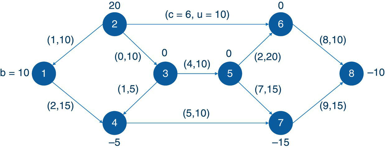
Figure 4.26 Network flow with costs and lower and upper bounds for nodes and links.
If the lower bound for the link is not defined, the algorithm assumes zero. If the upper bound is not defined, the algorithm assumes infinity. Similarly, for the nodes supply or demand, no value for the lower bound is assumed 0, and no value for the upper bound is assumed ∞.
To define a pure network, or a standard network flow problem, where the node supply must be met exactly, we can use the variable weight= only in the node's definition. Also, we don't need to specify all the node supply or demand bounds. For any missing node, the solver in proc optnetwork will use a lower and upper bound of 0.
An explicit upper bound of ∞ can be specified by using the special missing value “.I”. To explicitly define a lower bound of −∞, a special missing value “.M” is used.
Some constraints are applied to the algorithm. The flow on a link must be bounded from below. That means, a lower bound l ij = − ∞ cannot be used. The flow balance constraints cannot be free. That means, the lower bound for supply or demand ![]() and the upper bound for supply or demand
and the upper bound for supply or demand ![]() cannot be used.
cannot be used.
4.5.1 Finding the Minimum‐Cost Network Flow in a Demand–Supply Problem
Let us consider a very simple example to demonstrate the minimum‐cost network flow problem using proc optnetwork. Consider the graph presented in Figure 4.26. It shows a network with 8 nodes, 2 of them supplying goods, 3 of them demanding goods, and the remaining 3 not having any supply or demand constraints. Also notice that this is a pure network, a standard network flow problem. There are 2 nodes supplying 30 units in total (1 = 10 and 2 = 20), and 3 nodes demanding 30 units in total (4 = −5, 7 = −15 and 8 = −10). This balance will produce a perfect match in minimizing the cost to flow goods throughout the network. In this way, we have the nodes definition with the lower bound supply or demand specified. There is no definition for the upper bound, so it is set as infinity as default.
This network also shows the links. The links have the cost specified, and the upper bound definition. There is no lower bound specification, so it is assumed 0 as default.
The following code describes how to create the input datasets for the minimum‐cost network flow problem. Two datasets are created. The nodes dataset defines the lower bound for the supply or demand. Positive values set the supply and negative values set the demand. These values describe how much flow a node can send through at maximum and how much flow a node can receive at maximum. The links dataset defines the connections between the nodes, and for each connection, the cost to flow the goods on it and the upper bound, or the maximum flow that can be sent through on that particular link. Once again, there is no upper bound for the nodes, which means, they have infinity capacity, and there is no lower bound for the links, which means they have no minimum flow to be sent through.
data mycas.nodes;input node supdem @@;datalines;1 10 2 20 3 0 4 -5 5 0 6 0 7 -15 8 -10;run;data mycas.links;input from to cost max @@;datalines;1 4 2 15 2 1 1 10 2 3 0 10 2 6 6 10 3 4 1 5 3 5 4 104 7 5 10 5 6 2 20 5 7 7 15 6 8 8 10 7 8 9 15;run;
Once the input datasets are defined, we can now invoke the minimum‐cost network flow algorithm using proc optnetwork. The following code describes how to do it. Notice the links and nodes definition using the LINKSVAR and NODESVAR statements. For the links, the variable weight receives the cost to flow through that link and the variable upper receives the maximum that can be flowed. For the nodes, the variable lower receives the supply or demand values, which is the minimum that a node can send or receive in terms of flow.
proc optnetworkdirection = directedlinks = mycas.linksnodes = mycas.nodesoutlinks = mycas.linksoutmcnfoutnodes = mycas.nodesoutmcnf;linksvarfrom = fromto = toweight = costupper = max;nodesvarnode = nodelower = supdem;mincostflow;run;
Figure 4.27 shows the output for the minimum‐cost network flow algorithm. It says an optimal solution was found and the objective function (the minimal cost to flow goods through the network) is 270.
The following pictures show the minimum‐cost network results. The LINKSOUTMCNF dataset presented in Figure 4.28 shows the original variables, the from and to, which defines the link, the cost to flow throughout the link, and the upper bound, or the maximum allowed to be flowed throughout the link. The solution comes with the mcf_flow variable. It says how much should be flowed on each link to minimize the overall cost to flow all the goods. The variable mcf_rc presents the reduced cost for the optimal solution on each link.
Notice the reduced cost on each link. The reduced cost can be understood as the gain obtained by the optimal solution in minimizing the overall cost in flowing the goods throughout the network. Sometimes in pricing optimization, the reduced cost means the cost of buying something at node i, shipping it from i to j, and then selling it at j. For example, here the only way to flow something from node 1 to node 4 is exactly that link, from 1 to 4 . Then, there is no gain by flowing something using the link 1 to 4 . The reduced cost for this link is therefore 0. The cost to flow from 2 to 1 is 1. However, nothing was flowed using this link, so the reduced cost is 1. The cost to flow from 3 to 4 is 1. There is another way to flow things to 4 , through node 1 . But the cost to flow from 1 to 4 is 2. Then, the gain in flowing from 3 to 4 is −1. Let's take another example. The reduced cost for the link 4 to 7 is −4. The cost to flow from 4 to 7 is 5. Node 4 demands 5 and that was fulfilled through 3 . Node 4 also received 10 from node 1 at a cost of 2. Then the total cost to fulfill node 7 using node 4 is 7. There is another way to flow things to node 7 . All the way down from node 2 at cost 0, then from 3 to 5 at cost 5, and finally from 5 to 7 at cost 7. The total cost is 11. Then flowing through node 4 represents a gain of −4.
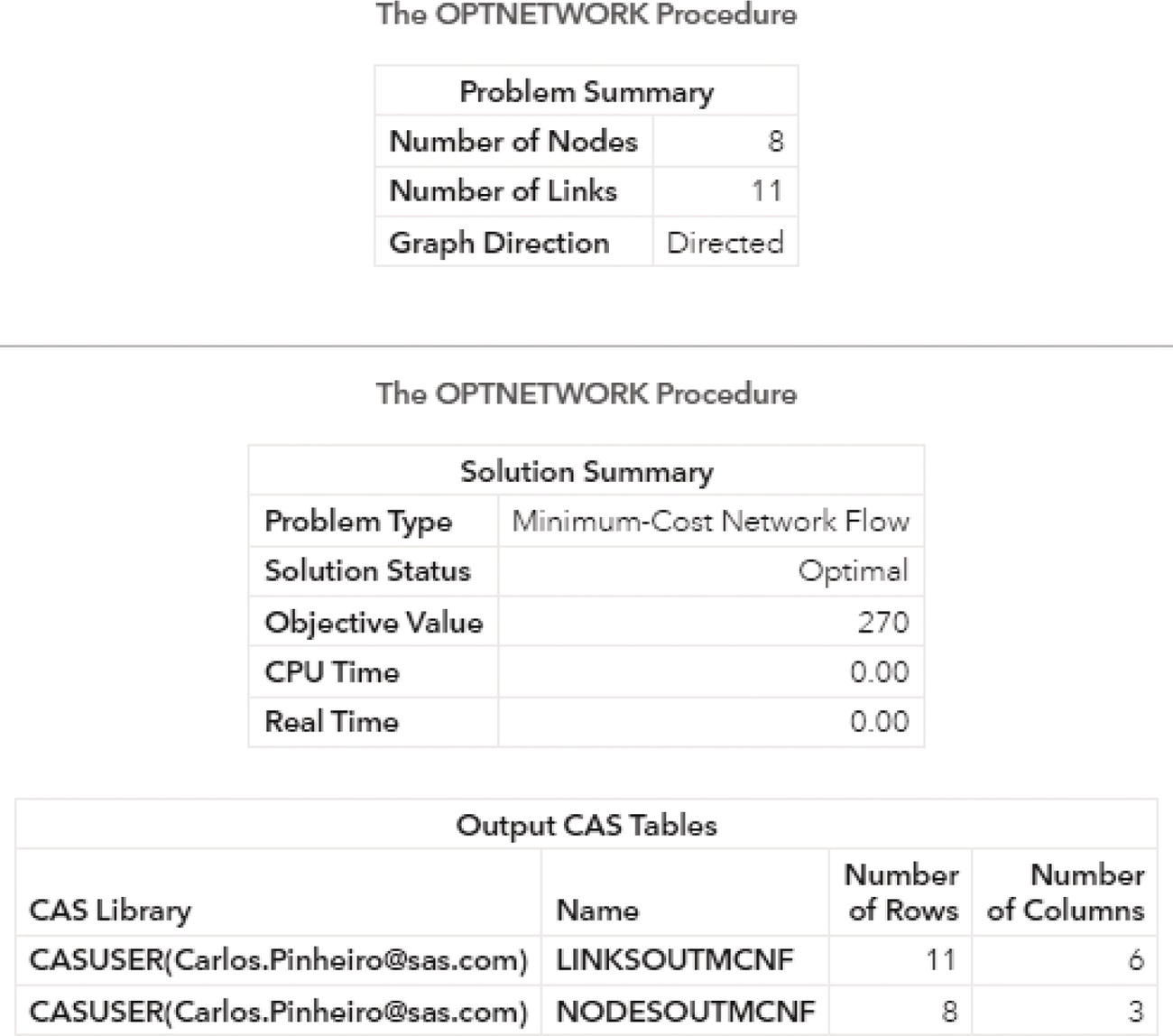
Figure 4.27 Output results by proc optnetwork running the minimum‐cost network flow algorithm.
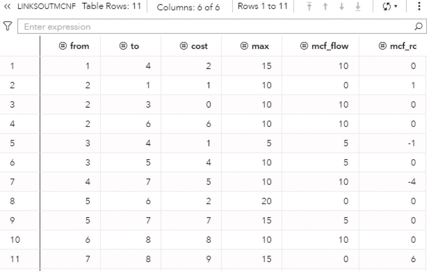
Figure 4.28 The minimum‐cost network flow solution for the links.
There is a solution report for the nodes as well. The NODESOUTMCNF dataset presented in Figure 4.29 shows the original variables, the node identification, and the supdem variable, which defines the lower bound for the supply or demand for each node to flow throughout the link. The variable mfc_dual presents the optimal dual value for the minimum cost network flow problem.
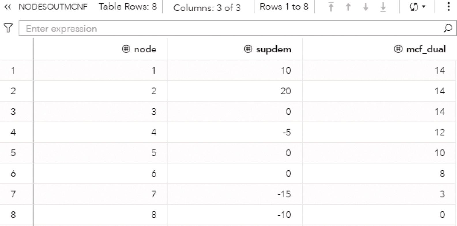
Figure 4.29 The minimum‐cost network flow solution for the nodes.
Notice the dual. The dual value is commonly used in price optimization. It is known sometimes as dual price. The optimal dual value is reported for each node in network flow problems. It gives the improvement in the objective function if the constraint is relaxed by one unit.
The dual values are computed during the iterations of the algorithm. The dual solution is used when the amount of flow is bounded on links within the network. The links within the network are either basic or non‐basic. The non‐basic links are limited at upper or lower bounds. Then, if the amount of flow between node i and j ![]() is basic, the cost is complementary for the dual values,
is basic, the cost is complementary for the dual values, ![]() . For example, the link between nodes 1 and 4 is basic, as the amount of flow is not limited at any upper or lower bound. The link between nodes 6 and 8 is non‐basic as the amount of flow is limited by the upper bound. The dual values are given by the basic links.
. For example, the link between nodes 1 and 4 is basic, as the amount of flow is not limited at any upper or lower bound. The link between nodes 6 and 8 is non‐basic as the amount of flow is limited by the upper bound. The dual values are given by the basic links.
Let’s set the dual value for node 8 is zero, ![]() . Then,
. Then, ![]() implies
implies ![]() . As
. As ![]() , we have for this link the following cost equation:
, we have for this link the following cost equation: ![]() , which is
, which is ![]() . Then the dual for the node 6 is 8. Going backwards in the network flow, the cost for the link between nodes 2 and 6 is 6:
. Then the dual for the node 6 is 8. Going backwards in the network flow, the cost for the link between nodes 2 and 6 is 6: ![]() , or
, or ![]() . Then, the dual for node 2 is 14. The process continues as the optimization algorithms run. There may be multiple sets of dual values as a result of the network simplex algorithm. Proc optnetwork searches for the optimal dual values.
. Then, the dual for node 2 is 14. The process continues as the optimization algorithms run. There may be multiple sets of dual values as a result of the network simplex algorithm. Proc optnetwork searches for the optimal dual values.
Figure 4.30 shows the solution for the minimum‐cost network flow problem, including the amount to flow for each link throughout the network.
The optimal solution defines a flow of 10 from 1 to 4, 10 from 2 to 3, 10 from 2 to 6, 5 from 3 to 4, 5 from 3 to 5, 10 from 4 to 7, 5 from 5 to 7, and finally 10 from 6 to 8.
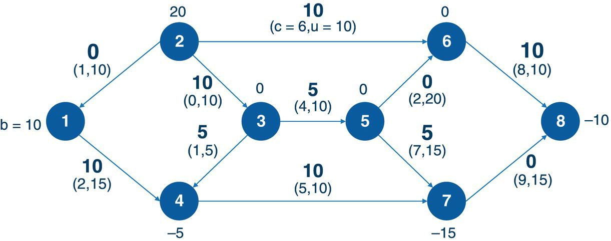
Figure 4.30 Minimum‐cost network flow results.
As stated before, this example describes a pure network, where the supply and demand are balanced. Considering all supplying nodes, the total supply is 30. Considering all demanding nodes, the total demand is also 30.
Let's consider now a more flexible example. Nodes may have an infinity or huge capacity or can have a range in the lower and upper bounds. For example, nodes may supply in a particular range, from 10 to 100, or can have a flexible demand, from 10 to 20.
The following code defines a more flexible network considering the exact same topology. Here, some nodes have a range in supply or demand, including infinity supply and demand values. Analogously, the links also have a range in the lower and upper bound for the amount of flow.
data mycas.nodes;input node min max @@;datalines;1 10 .I 2 0 40 3 0 0 4 -10 -55 0 0 6 0 0 7 .M -10 8 -50 -20;run;data mycas.links;input from to wgt min max @@;datalines;1 4 2 5 10 2 1 1 0 10 2 3 0 5 20 2 6 6 10 20 3 4 1 5 5 3 5 4 0 104 7 5 10 10 5 6 2 0 20 5 7 7 5 15 6 8 8 0 10 7 8 9 0 15;run;
The following code describes how to invoke proc optnetwork to search for the minimum‐cost network flow considering this new scenario. Notice the definition of links and nodes to specify lower and upper bounds for supply or demand, and amount of flow.
proc optnetworkdirection = directedlinks = mycas.linksnodes = mycas.nodesoutlinks = mycas.linksoutmcnfoutnodes = mycas.nodesoutmcnf;linksvarfrom = fromto = toweight = wgtlower = minupper = max;nodesvarnode = nodelower = minupper = max;mincostflow;run;
Figure 4.31 shows the output for the minimum‐cost network flow algorithm. It says an optimal solution was found and the objective function was 415.
Let's take a look at the results. The LINKSOUTMCNF dataset presented in Figure 4.32 shows the mcf_flow variable with the amount of flow to be sent throughout the network. It says how much should be flowed on each link to minimize the overall cost to flow all the goods. The variable mcf_rc presents the reduced cost for the optimal solution on each link.
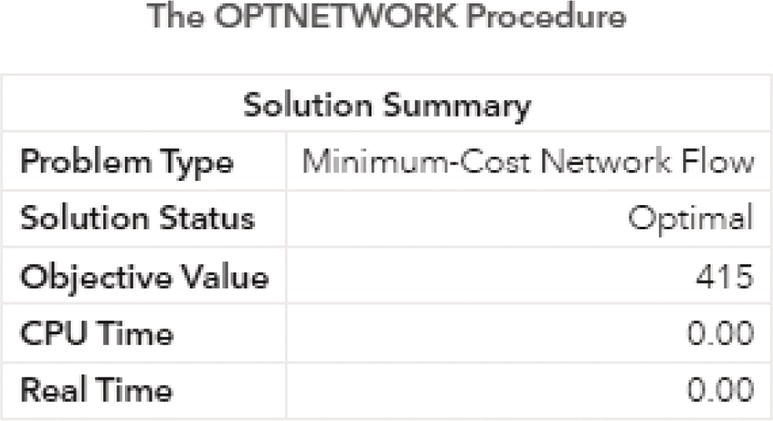
Figure 4.31 Output by proc optnetwork running the minimum‐cost network flow algorithm for a flexible network problem.
The major difference in relation to the previous solution are the links 2–3 , 3–5 , 5–7 , and 7–8 . As node 8 demands more units, now those links are flowing the amount of 15, 10, 10, and 10, respectively.
Figure 4.33 shows the solution for the minimum‐cost network flow problem considering this flexible network.
The figure with the solution flow suppresses the information about the links, like the cost to flow throughout the link, and the lower and upper bounds of possible amount to be flowed by using the link. It shows only the information about the range of the supply and demand for the nodes, and the optimal amount of flow as a solution.
Finally, suppose that node 8 requires a range of −100 and −50 units, as described in the following code. The other nodes are suppressed to simplify the explanation, but they are in the original data step that creates the nodes dataset.
data mycas.nodes;input node min max;datalines;8 -100 -50;run;
Even though some nodes can dispatch loads of units, with node 1 producing an infinity amount, the links are limited by upper bounds. The amount required by node 8 cannot be accomplished. On this case, proc optnetwork returns that there is no feasible solution for this problem. Figure 4.34 shows the summary results from proc optnetwork.
One way to overcome this limitation is to increase the possible number of units that can be flowed through the links 1–4 , 4–7 , and 7–8 . We can increase the upper bound limits or just make them infinity, as shown in the following code:
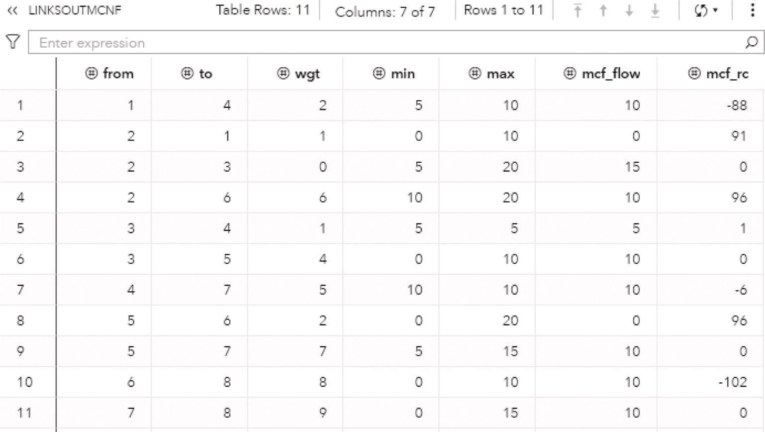
Figure 4.32 The minimum‐cost network flow solution for the links.
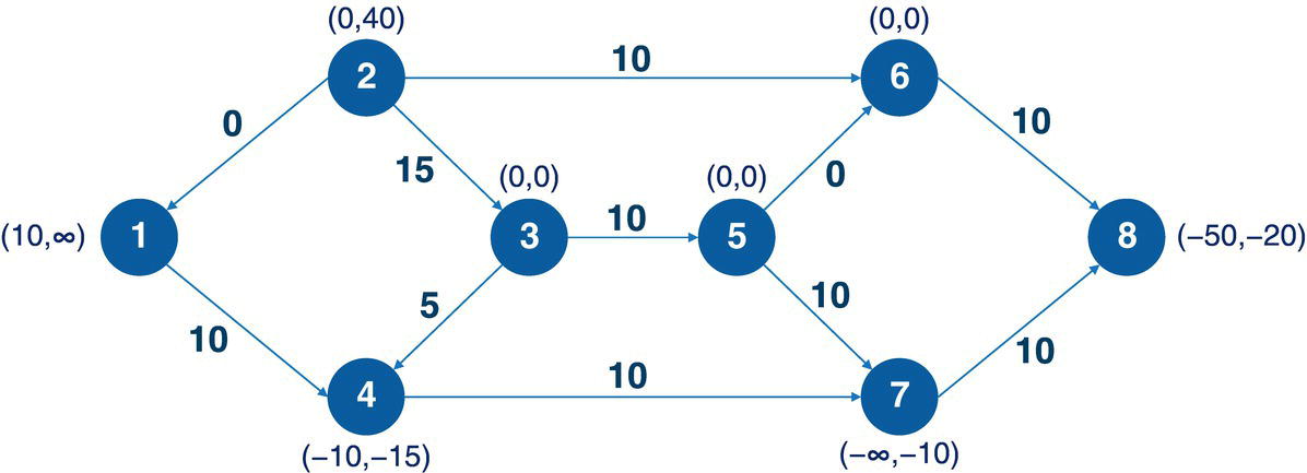
Figure 4.33 Minimum‐cost network flow results for the flexible network.
data mycas.links;input from to wgt min max;datalines;1 4 2 5 .I...4 7 5 10 .I...7 8 9 0 .I;run;
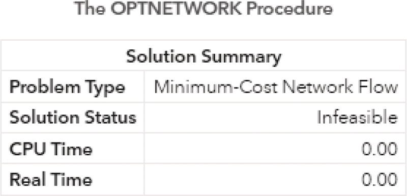
Figure 4.34 Output by proc optnetwork showing that there is no feasible solution for the network flow problem considering the constraint for node 8.
Increasing the number of units that can be flowed throughout these links allows for a feasible solution. Proc optnetwork shows that an optimal solution can be found, and the objective function is 875. Figure 4.35 shows the summary results with the objective value.
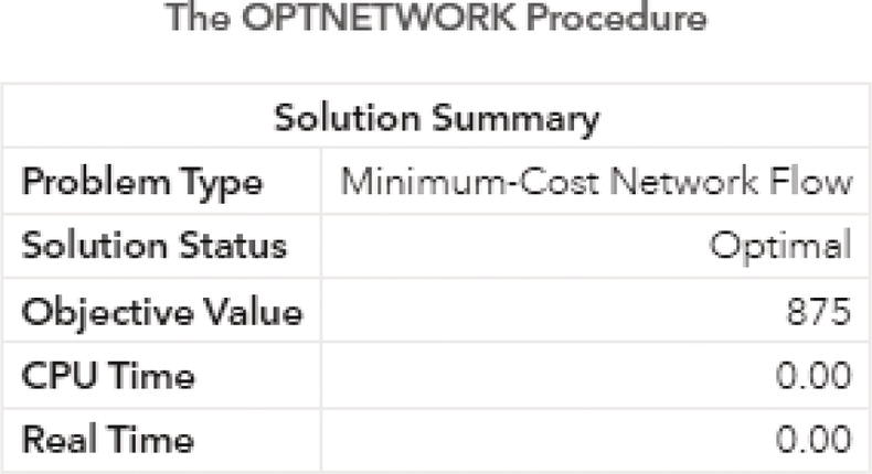
Figure 4.35 Output by proc optnetwork showing a feasible solution for the network flow problem considering the increase in the upper bound for some links.
For more complex scenarios in network flow problems, there is a SAS procedure called OPTLP that can be used. Proc OPTLP provides four methods for solving linear programs, including primal simplex algorithm, dual simplex algorithm, network simplex algorithm (similar to the mincostflow algorithm in proc optnetwork), and interior point algorithm.
4.6 Maximum Network Flow Problem
In optimization theory, maximum flows problems involve finding a feasible flow throughout a flow network that obtains the maximum possible flow rate. In graph theory, a flow network is defined as a directed graph involving a source node s and a sink node t, along several other nodes connected by multiple links. Each ink has an individual capacity, which is the maximum limit of flow that the link could allow. The feasible flow is a single source and a single sink flow network that is maximum.
Let’s assume G = (N, L) is a directed graph. For each link ij ∈ L, we define a nonnegative capacity u ij that specifies the maximum flow that link ij can carry. We also define decision variables x ij that denote the amount of flow sent across each link ij. The problem can be modeled as a linear programming problem as:
where ![]() represents the set of outgoing links that are connected from node i, and
represents the set of outgoing links that are connected from node i, and ![]() represents the set of incoming links that are connected to node i.
represents the set of incoming links that are connected to node i.
In proc optnetwork, the MAXFLOW statement invokes the algorithm that solves the maximum network flow. The input for the network flow is a standard graph input. If the input is an undirected graph, then proc optnetwork treats each link as two directed links with the same capacity. Proc optnetwork uses the Boykov‐Kolmogorov algorithm to compute the maximum flow.
There are only two options for the maximum network flow algorithm in proc optnetwork. The first option is to define the source node of the network flow. The option SOURCE= specifies the node where the flow starts for the maximum network flow calculations. The option SINK= specifies the node where the flow ends for the maximum network flow calculations.
The final result for the maximal network flow algorithm is reported and saved in output tables defined by the OUTLINKS= and OUTNODES= options. The resulting optimal flow for the maximal network flow algorithm through the network is saved on the output table specified in the OUTLINKS= option. This output table includes the original information on the links dataset, which is the from node, the to node, and the upper limit to be flowed on the link, plus the optimal flow for each link, stored in the variable called mf_flow. If the output table for the nodes is specified in the OUTNODES= option, it stores just the list of nodes within the network.
The definition of the links in the maximal network flow algorithm is crucial. It defines the constraints for the network flow problem and how the algorithm will search for the optimal solution. The links dataset is defined using the LINKS= option. For the maximal network flow, the nodes dataset doesn't need to be defined. We can do it, but it doesn't impact the algorithm. The DIRECTION= option can be specified as directed or undirected. If the graph is directed, the links direction follows the links definition, which means, if we have a link A‐B with an upper limit of 10, that would be a direct link departing from A, arriving at B, and allowing a maximal flow of 10 units. If the graph is undirected, each link is defined in both directions with the same upper limit. The previous case would turn into 2 links, from A to B with an upper limit of 10, and a second link from B to A with the same upper limit of 10 units. In the LINKSVAR statement, the variables from= and to= are used to define the link x ij , and the variable upper= is used to define the upper limit u ij for the link to flow.
Notice that differently than the minimum cost network flow problem, unlimited bounds are not allowed. The explicit upper bound of ∞ cannot be specified by using the special missing value “.I”. The link must have a finite upper limit to be flowed.
4.6.1 Finding the Maximum Network Flow in a Distribution Problem
Let's consider a simple example to demonstrate the maximum network flow problem using proc optnetwork. Consider the graph presented in Figure 4.36. It shows a network with 8 nodes and 12 links. This network is represented by a directed graph, where the direction of the link matters. Each link has a maximum capacity to flow through the network. The departing node will be node A, and the arriving node will be node H. The maximum network flow algorithm searches for the optimal solution, aiming for the maximum units to be flowed in each link from node A throughout node H.
The following code describes how to create the input dataset for the maximum network flow problem. In the previous algorithm, the minimum cost network flow problem, two datasets needed to be created, one for the nodes and another one for the links. These two datasets define all the constraints and resources assigned to the problem. The maximum network flow problem is simpler. It requires only the links dataset, containing a single constraint which is the upper limit capacity to be flowed in each link.
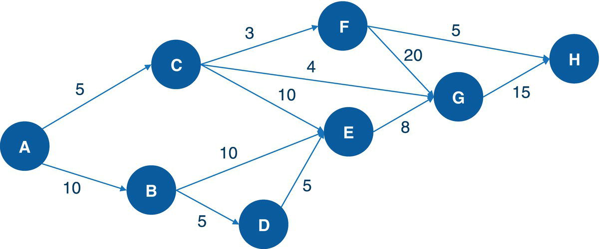
Figure 4.36 Network flow with upper limits of flow in each link.
data mycas.links;input from $ to $ max @@;datalines;A B 10 A C 5 B D 5 B E 10 C E 10 C F 3C G 4 D E 5 E G 8 F G 20 F H 5 G H 15;run;
Once the input dataset is created, now we can invoke the maximum network flow algorithm using proc optnetwork. The following code describes how to do it. Notice the links definition using the LINKSVAR statements. Like all the other examples, the variables from= and to= define the link, and the variable upper= define the maximum capacity to be flowed in the link. The option DIRECTION= defines in this particular case that the network is a directed graph. When invoking the maximum network flow algorithm, both source and sink nodes must be defined. Here, node A is the starting point for the maximum network flow problem, and node H is the ending point. They are defined using the options SOURCE= and SINK= in the maxflow algorithm.
proc optnetworkdirection = directedlinks = mycas.linksoutLinks = mycas.linksoutmnf;linksvarfrom = fromto = toupper = max;maxflowsource = 'A'sink = 'H';run;
Figure 4.37 shows the output for the maximum network flow algorithm. It says an optimal solution was found and the objective function (the maximum units to be flowed from the starting point A throughout to the ending point H) is 13.
The following picture shows the result table for the minimum network flow algorithm. The LINKSOUTMNF dataset presented in Figure 4.38 shows the original information on the links, the from and to variables that define the link (origin and destination), the max variable, which defines the upper limit to be flowed on that link. The solution comes with the mf_flow variable. It says how much should be flowed on each link to maximize the amount of flow throughout the network departing from node A and arriving at node H.
The output table has all the links of the network flow, with the amount of flow to be flowed on each link. The output table includes even the links that are not used to send any flow. There are four links with no flowed, B‐D, C‐E, D‐E, and F‐G. All of them have a maximum capacity to flow something but they were not used to flow anything. Their mf_flow is zero. Five links flow less amount than their maximum capacity. The links A‐B, B‐E, C‐G, F‐H, and G‐H flow 8 out of 10, 8 out of 10, 2 out of 4, 3 out of 5, and 10 out of 15, respectively. Finally, three links flow their maximum capacity. The links A‐C, C‐F, and E‐G flow 5 out of 5, 3 out of 3, and 8 out of 8, respectively.
Figure 4.39 shows the solution for the maximum network flow problem, including the amount to flow for each link throughout the network, starting at node A and ending at node H.
Starting from the top of the network, the optimal solution defines a flow of 5 from A to C, then a split flow of 3 from C to F, and 2 from C to G. The flow of 3 from C to F continues from F to H, the destination. From the bottom part of the network, there is a flow of 8 from A to B, and then that amount of flow continues from B to E, and from E to G. Node G now has received 2 flows from C and 8 flows from E. Node G sends those 10 flows to H, the final destination node. With the 3 flows sent from F, node H receives the total flow of 13, the same amount initially sent by node A, the starting point of the network flow.
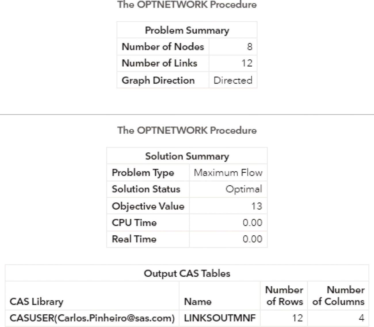
Figure 4.37 Output results by proc optnetwork running the maximum network flow algorithm.
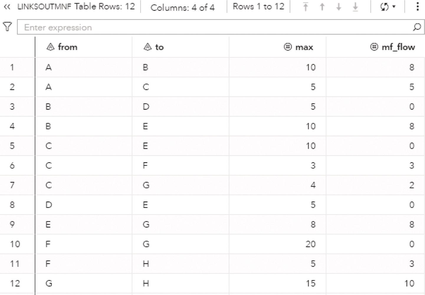
Figure 4.38 The maximum network flow solution for the links.
Notice that the maximum flow depends on the entire network and the maximum capacity for all the links. The maximum amount of flow starting from node A is 15, considering 5 through the link A‐C and 10 through the link A‐B, the maximum flow in this scenario is 13. However, even if we increase the upper limit for these initial links, the maximum flow still relies on the rest of the flow, either in the middle of the network or at the end of the flow. For example, even if we get a substantial increase in these first two links, the maximum flow still doesn't get much better as the maximum to be flowed to node H is 15. Even though node H can receive 20 units (5 from F and 15 for G), node F can receive just 3 (from C) and node G just 12 (4 from C and 8 from E). Based on that, the maximum network flow for this graph would be 15 on top.
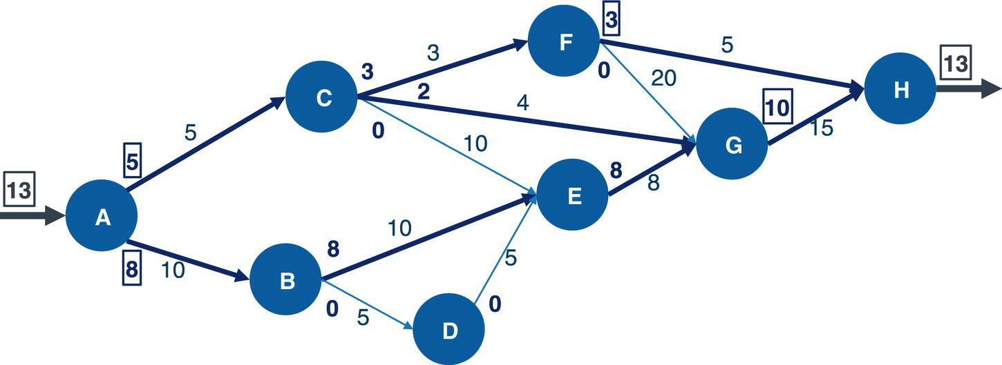
Figure 4.39 Maximum network flow results.
Let's change for example the upper limit for the first two links
data mycas.links;input from $ to $ max;datalines;A B 100A C 100...;run;
Figure 4.40 shows that the objective value for the maximum network flow algorithm is now 15.
One of the great benefits from the maximum network flow algorithm is to search for the overall optimal solution. The amount to be flowed on every link is considered in order to optimize the network flow. That means, even though some links can flow more units, there is no reason to do so if the following nodes in the consecutive steps cannot accommodate that amount. Then, the optimal solution minimizes the amount of flow throughout the entire network to achieve the maximum network flow to reach out to the final destination.
For example, let's consider that new example, where the first two links have a limit capacity of 100 units. Let's assume we flow the maximum capacity at all times. Figure 4.41 presents a possible solution for this maximum network flow problem.
The process starts flowing 200 from A (100 to C and 100 to B), then from C to F there is a flow of 3, to G a flow of 4, and to E a flow of 10. Here the losses begin because of the limit capacity in the following links. Even though C receives 100, it can flow only 17 in total. The same case for B. It flows 10 to E and 5 to D. Again, B receives 100 and flows forward only 15. By now, 166 units were flowed from A to B and C for nothing as they couldn’t be flowed forward (83 at C and 85 at B). From D there is a flow of 5 to E. Here there is another small waste. E receives 15 but can flow forward just 8. In addition to the 166 units that flowed before, another 7 were flowed for no reason. The last 2 steps are optimal. F has 3 units, can send 5 to H, and send those 3. G has 12 units, can send 15 H, and send those 12. In this way, the final node H receives 15. However, considering this approach there were 173 units flowed across the network for no reason. If we imagine that there is no cost to send units throughout the network, this is not a big deal. But there is no lunch free. Everything has a cost, and in real world optimization problems, sending units throughout a network flow certainly has a cost associated with it. Then, the optimal flow should account for that, minimizing the number of units sent through to achieve the maximum flow from the origin node to the destination node.
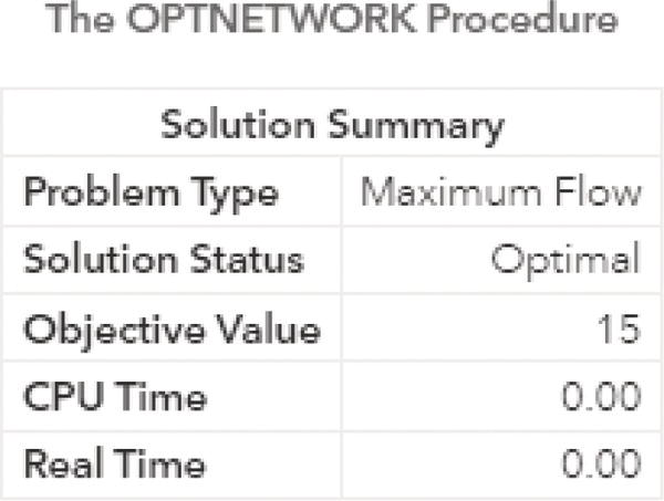
Figure 4.40 Output results by proc optnetwork running the maximum network flow algorithm.
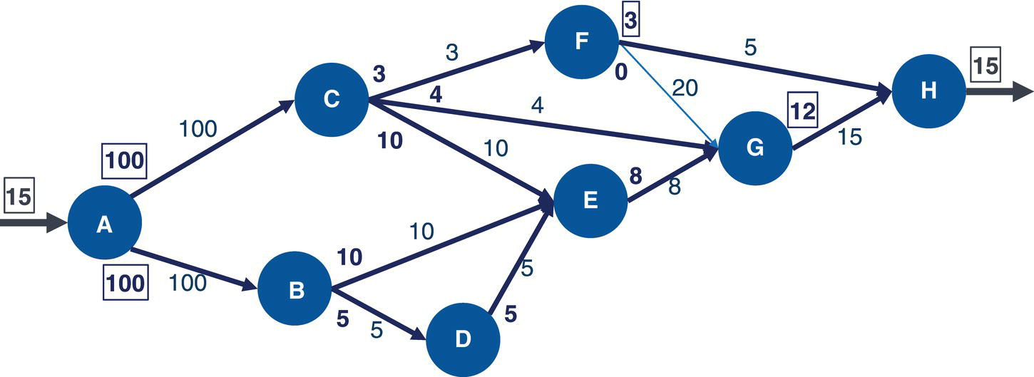
Figure 4.41 Maximum network flow results.

Figure 4.42 Maximum network flow results.
The optimal solution for the case we have increased the maximum capacity for the first 2 links as shown in Figure 4.42.
The optimal solution considers sending just the number of units that will be flowed forward by the consecutive nodes within the network flow. That approach would save the cost of sending units throughout the network for no reason. In order to increase the maximum network flow, it is necessary to increase the upper limit for some of the links in the middle of the network, like C‐F, F‐H, and E‐G.
4.7 Minimum Cut
In graph theory, cut is a partition of the nodes of a graph into two disjoint subsets. The subsets are formed minimizing some particular metric. The minimum cut problem can be applied to both directed and undirected networks. If two terminal nodes are specified, they are commonly referred to as source and sink nodes. In a directed graph, the minimum cut separates the source and sink nodes by minimizing the total weight on the links that are directed from the source side of the cut to the sink side of the cut.
The minimum cut problem has many applications in areas such as network design. The minimum cut problem has two variants in terms of definitions. The first one is assigned to find the minimum set of links that if removed disconnects a particular node s from a particular node t. This variant of the problem is called the minimum s‐t cut problem. The second variant is assigned to find the minimum set of links that if removed disconnects the graph. The variant is called the minimum cut problem. SAS proc optnetwork addresses both variants of the problem, for directed and undirected graphs.
A cut is a partition of the nodes N of a graph G = (N, L) into two disjointed subsets S and T = NS. The cut S is a proper subset of N, where S ⊂ N and S ≠ ∅ , N. The size of the cut with respect to S is the number of links between S and the rest of the graph NS. A cut set is the set of links that join a node in S to a node in T. In a regular network, we can find lots of cut sets. A minimum cut of a graph is a cut whose cut set has the smallest link metric. The link metric can be measured by distinct methods. For example, in unweighted graphs, the link metric can be the number of links in the cut set. On the other hand, in weighted graphs, the link metric can be the sum of the link weights in the cut set.
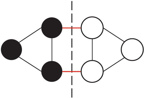
Figure 4.43 Image in pixels represented by nodes and links.
Another common application of the minimum cut problem nowadays is on image segmentation. Suppose we have an image created by a multitude of pixels. Imagine that we want to partition that image into two disjointed parts, or two dissimilar portions of the original image. We can turn the pixels of the image into nodes within a graph. The links will be added to connect similar pixels, or nodes within the graph. The minimum cut will represent a partition of the pixels where two portions of the image are most dissimilar. Figure 4.43 shows a representation of this graph.
The size of the cut in this image representation is 2, represented by the two links in red in the middle of the graph. These links partition the graph into two disjointed portions, the black nodes, and the white nodes.
In proc optnetwork, the MINCUT statement invokes the algorithm that solves the minimum‐cut problem. The algorithm solves both variations described before. The first one, the minimum s‐t cut problem, requires that the source and sink nodes be defined, and the network must be specified as a directed graph. The second variant, the minimum cut problem, runs for the entire network. The source and sink nodes cannot be defined and the network needs to be defined as an undirected graph.
There are few options for the minimum cut algorithm in proc optnetwork. They are very important in defining the problem the algorithm will search as an optimal solution. The MINCUT statement invokes an algorithm that finds the minimum link‐weighted cut of an input graph. The first option is assigned to the number of cuts. The option MAXCUTS= specifies the maximum number of cuts for the algorithm to return. The minimal cut and any other cut that are found during the optimal search executed by the algorithm are returned, up to the number specified in the option. By default, the maximum number of cuts returned by the algorithm is one. The resulting minimum cuts are described in terms of nodes and links. For the nodes, the algorithm returns the partitions of the nodes within the graph. For the links, the algorithm returns the links in the cut sets. The partition of the nodes within the graph is specified in the output table by the variable partition. Each cut within the graph is identified in the output table by the variable cut. Then, for each cut, the algorithm returns an identifier for the cut and an identifier for the partition. Each node will be assigned to a value 0 or 1, defining if the node, that that particular cut, belongs to the node set S or to the node set T. The algorithm also produces an output table containing the cut sets. This table lists the links and their weight for each cut identified.
The second option refers to how the algorithm account for the weights of the links when creating the cut sets. The option MAXWEIGHT= specifies the maximum weight of the cuts to be returned by the algorithm. Only cuts whose weight is less than or equal to the number specified in the option are returned by the algorithm. The default is the largest number that can be represented by a double. That basically means that there is no limit to the total weight for the links creating the cut sets. All cut sets will be returned by the algorithm if the option is not specified.
The final result for the minimum cut algorithm in proc optnetwork is reported in the output tables specified in the options OUTCUTSETS= and OUTPARTITIONS=. The option OUTCUTSETS= specifies the output data table that contains the minimum cut sets to the minimum‐cut problem. This output table contains the variable cut identifying the cut set, and the original variables from, to, and weight describing the links, which create the partitions. The option OUTPARTITIONS= specifies the output data table that contains the minimum cut partitions to the minimum‐cut problem. This output table contains the variable cut identifying the cut, the original node identifier, and the partition identifying if the node either belongs to the node set S or to the node set T.
The options described before are mostly assigned to the second variation of the minimum cut problem, where the minimum set of links to disconnect the graph is searched. That problem is associated with undirected graphs. The first variation of the minimum cut problem is assigned to find the minimum set of links that disconnects a particular node from one partition or set S to another partition or set T. The following options are associated with that variation, called the minimum s‐t cut problem.
The option SINK= specifies the sink node for minimum s‐t cut calculations. If this option is specified, the option SOURCE= must be specified too. The option SOURCE= specifies the source node for minimum s‐t cut calculations. Analogously, if this option is specified, the option SINK= must be specified as well. When these options are specified, the MINCUT algorithm in proc optnetwork solves the minimum s‐t cut problem. The cut set in this problem intersects every path from the source node s specified in the option SOURCE= to the sink node t specified in the option SINK=. These options also imply that the graph is directed, as the cut partitions the links starting from node s ending at node t. Finally, the algorithm to solve the minimum s‐t cut problem returns only one cut.
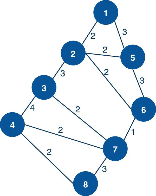
Figure 4.44 Undirected graph with weighted links.
The MINCUT statement in proc optnetwork uses the Stoer‐Wagner algorithm to compute the minimum cuts.
4.7.1 Finding the Minimum Cuts
Let's consider a simple example to demonstrate the minimum cut problem using proc optnetwork. Consider the graph presented in Figure 4.44. It shows a network with 8 nodes and 12 links. The network is represented by undirected links. All links within the network have weights, that will be used in searching for the minimum cuts.
The following code describes how to create the input dataset for the minimum cut problem. Notice that just the links dataset is required. The links dataset identifies the connections between all the nodes within the graph, and for each connection, it defines the respective weight, which will be accounted for when proc optnetwork calculates the minimum cuts.
data mycas.links;input from to weight @@;datalines;1 2 2 1 5 3 2 3 3 2 5 2 2 6 2 3 4 43 7 2 4 7 2 4 8 2 5 6 3 6 7 1 7 8 3;run;
Once the input dataset is defined, we can now invoke the minimum cut algorithm using proc optnetwork. The following code describes how to invoke the minimum cut statement to calculate the minimum cut sets within the graph. Notice the links definition using the LINKSVAR statement to define the links (from and to variables) and the weight for each link (weight variable).
proc optnetworkdirection = undirectedlinks = mycas.links;linksvarfrom = fromto = toweight = weight;minCutoutcutsets = mycas.cutsetsoutpartitions = mycas.partitionsmaxcuts = 10;run;
Notice that it is still possible to define the output tables using the options OUTLINKS= and OUTNODES=. However, these options here have no effect on the output results. The output table specified in the option OUTLINKS= will be exactly the same as the links dataset, containing all the links and weights identified by the variables form, to, and weight. The output table specified in the option OUTNODES= will have only the list of the nodes identified by the variable node. The output tables with the results produced by proc optnetwork when searching for the minimum cut sets are saved through the options OUTCUSETS= and OUTPARTITIONS=.
Figure 4.45 shows the output for the minimum cut algorithm. It says an optimal solution was found and the objective function equals to 4. There is also information about the number of links and nodes in the original dataset, and the number of rows and columns in the output datasets.
The following picture shows the minimum cut results. The PARTITIONS dataset presented in Figure 4.46 shows the cuts, containing all disjoint partitions or disjoint sets of nodes. The variable cut indicates the cut, the variable node indicates which node belongs to that cut set, and the variable partition indicates in which partition the node belongs, either to the node set S or to the node set T.
The CUTSETS dataset presented in Figure 4.47 shows the cut sets, with the links creating the disjoint partitions within the graph. The variable cut identifies the cut set, and the original variables from, to, and weight identify the links creating the disjoint partitions.
Notice that we have seven partitions. The CUTSETS dataset identifies the links that create these partitions, and the PARTITIONS dataset identifies the nodes in each partition. Figure 4.48 shows all the seven minimum cut sets identified by proc optnetwork considering the input graph.
Also notice that, even though we have specified a maximum of 10 minimum cuts to be found (MAXCUTS = 10), proc optnetwork has found only 7 cuts, and then all these cuts were reported to the final results. Large networks are likely to have a great number of minimum cuts. A good approach is always to start small in terms of the number of cut sets to be reported in the final result and then increase progressively the maximum number of cuts in the output table.
The previous example describes the minimum cut problem based on an undirected graph. As we saw before, there are two variants for the minimum cut problem. The first one is the minimum s‐t cut problem and the second one is the minimum cut problem. Let's take a look at the minimum s‐t cut problem. Assume the same network we have used for the minimum cut problem. Now, for the minimum s‐t cut problem, we need to define the source and sink nodes and make the graph to be directed. The graph with directed links is presented in Figure 4.49.
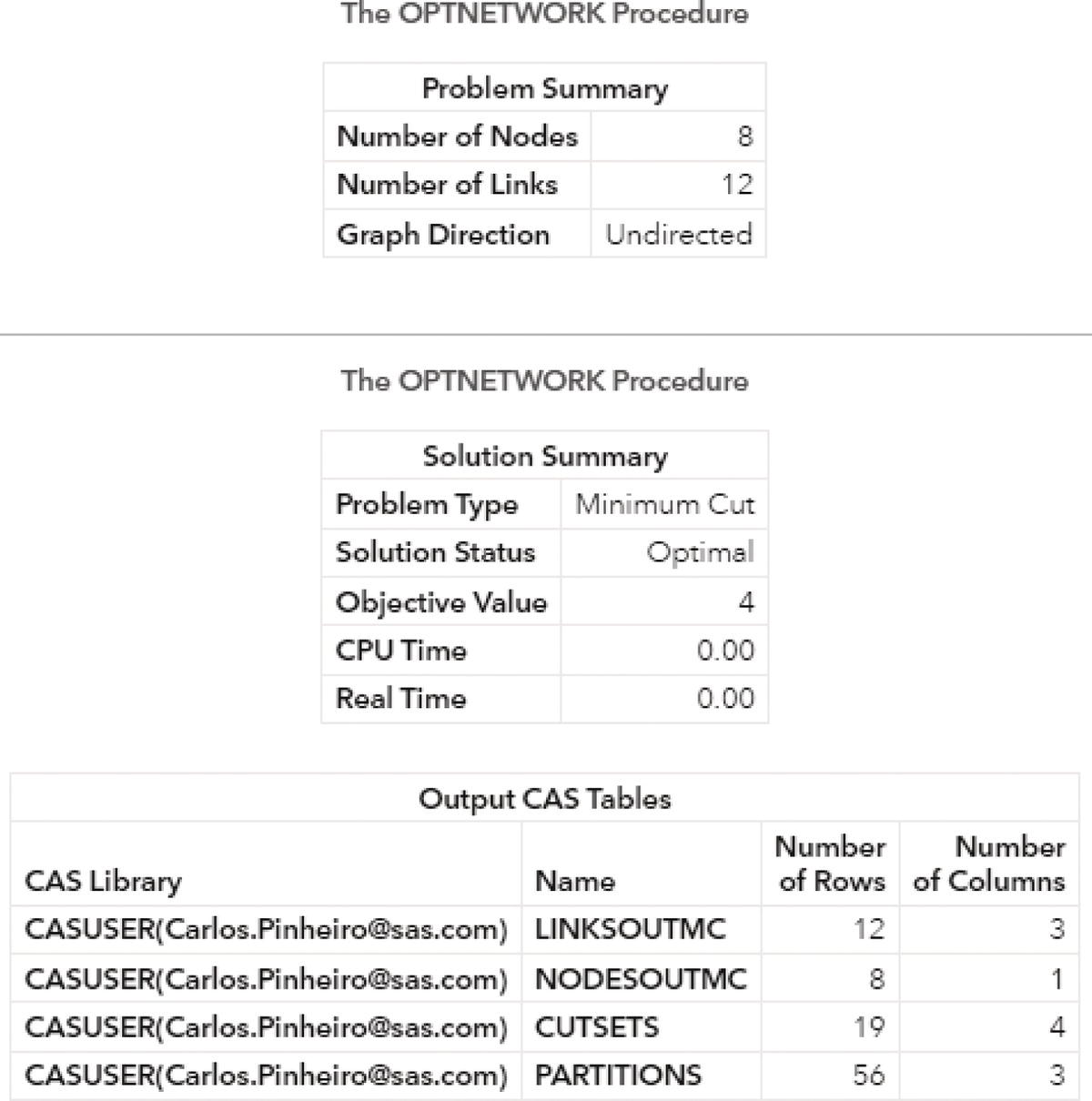
Figure 4.45 Output results by proc optnetwork running the minimum cut algorithm.
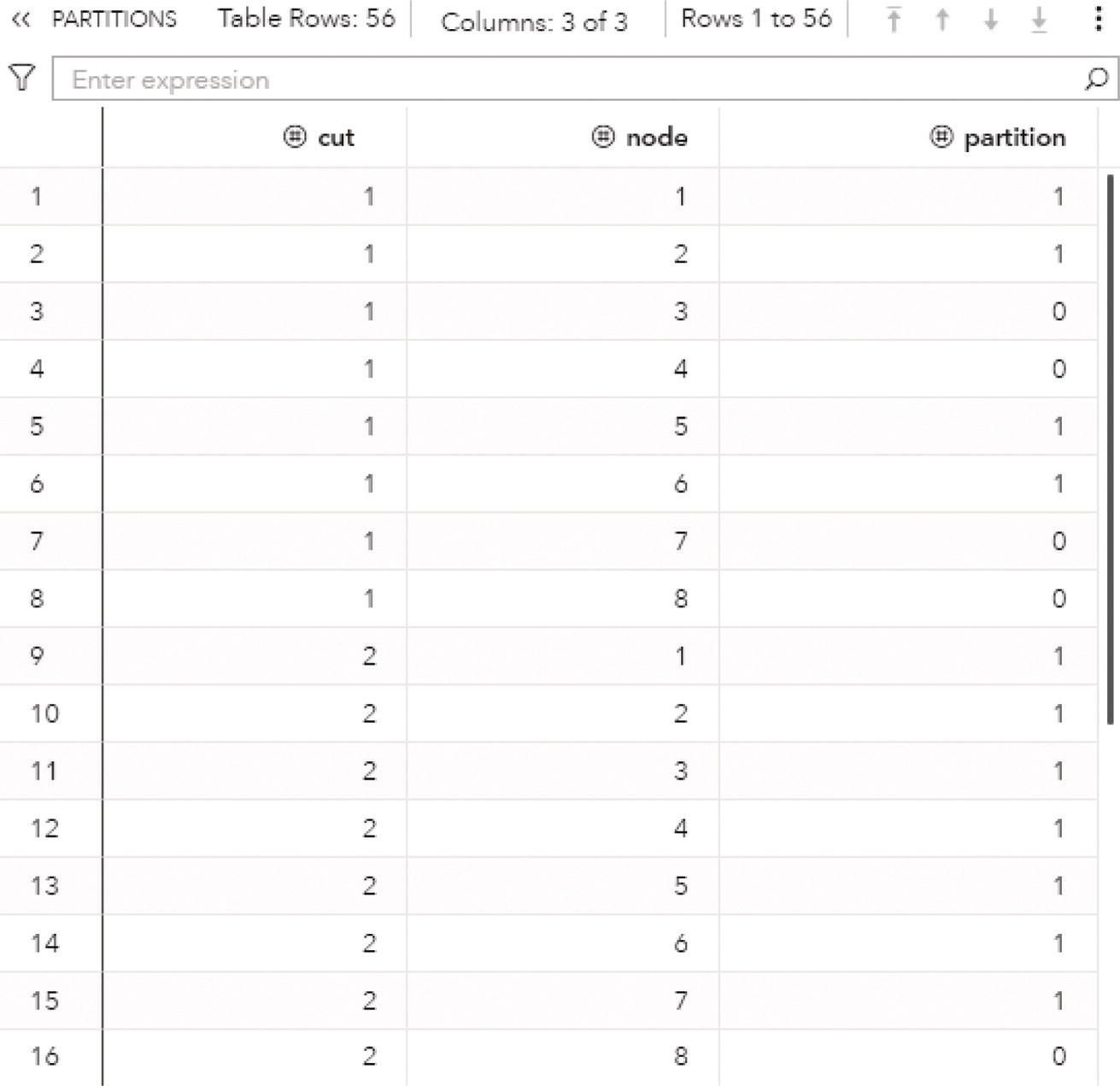
Figure 4.46 Result table for the partitions in the minimum cut problem.
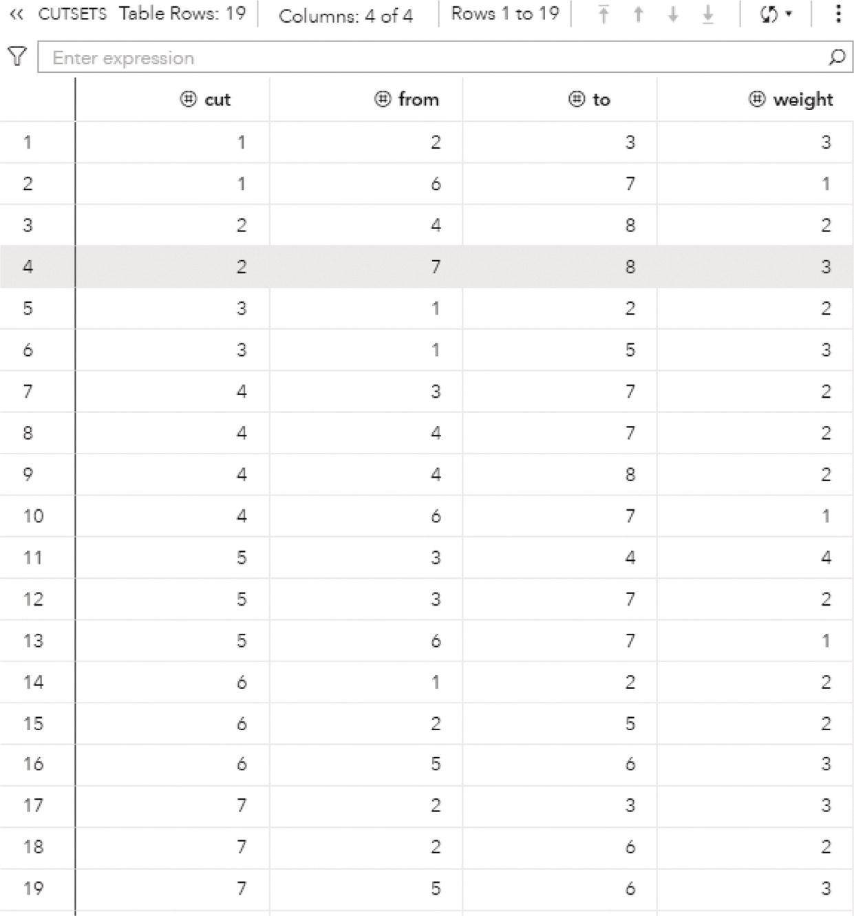
Figure 4.47 Results table for the cut sets in the minimum cut problem.

Figure 4.48 Minimum cut sets for the input graph.

Figure 4.49 Directed graph with weighted links.
Let's also assume the node 1 as the source node and node 8 as the sink node. The following code defines these constraints and invoke the minimum cut algorithm to execute on the directed graph.
proc optnetworkdirection = directedlinks = mycas.links;linksvarfrom = fromto = toweight = weight;minCutoutcutsets = mycas.cutsetsoutpartitions = mycas.partitionssource = 1sink = 8;run;
The following picture shows the minimum s‐t cut results. The PARTITIONS dataset presented in Figure 4.50 shows that there is one single minimum s‐t cut, splitting the 8 nodes into 2 partition of 4 nodes each. The partition indicates as 0 or 1 in which partition each node belongs, either to the set S or to the set T.
The CUTSETS dataset presented in Figure 4.51 shows the links that create the cut sets. For this particular network, considering a directed graph and the source node as the node 1 and the sink node as the node 8, there are just 2 links that partition the graph into 2 sets of nodes.
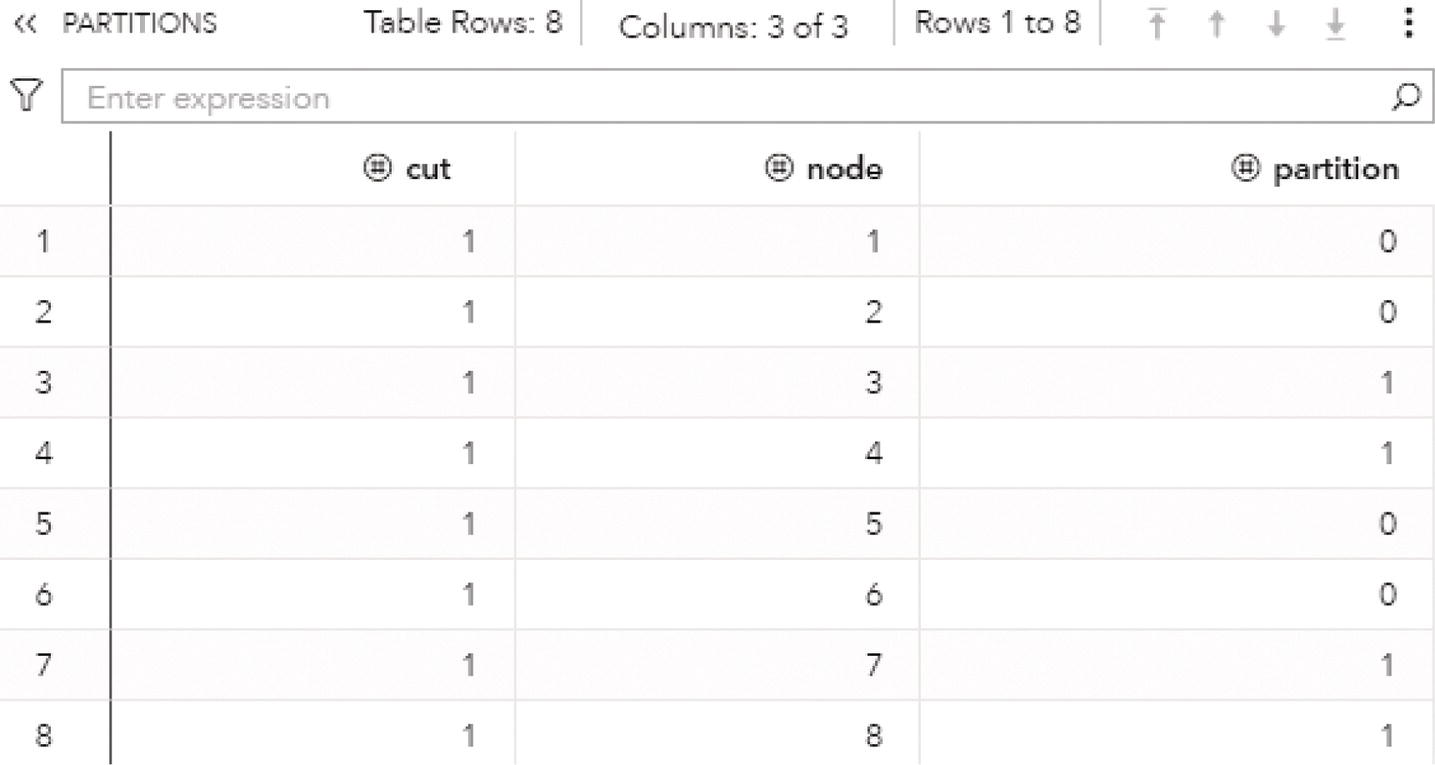
Figure 4.50 Result table for the partitions in the minimum s‐t cut problem.
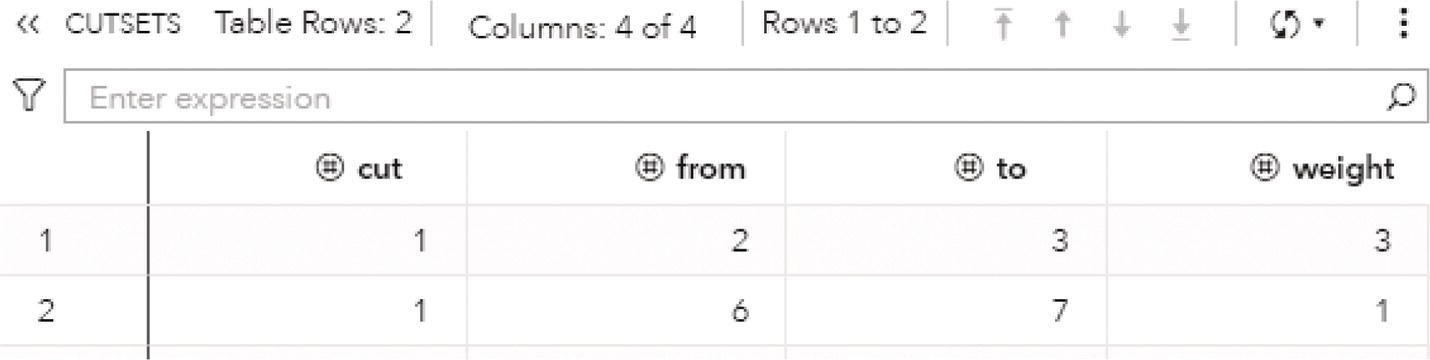
Figure 4.51 Results table for the cut sets in the minimum s‐t cut problem.
The minimum s‐t cut, and the 2 disjoint partitions are represented in Figure 4.52. The cut set are the 2 links in bold red. The cuts are the 2 groups of nodes identified in light and dark blue.
Node 1 is the source node, the s node of the set S, which comprises nodes 1, 2, 5, and 6. Node 8 is the sink node, the t node in the set T, which comprises nodes 3, 4, 7, and 8. The minimum s‐t cut problem is defined by the cut set comprising the links 2‐3 and 6‐7.
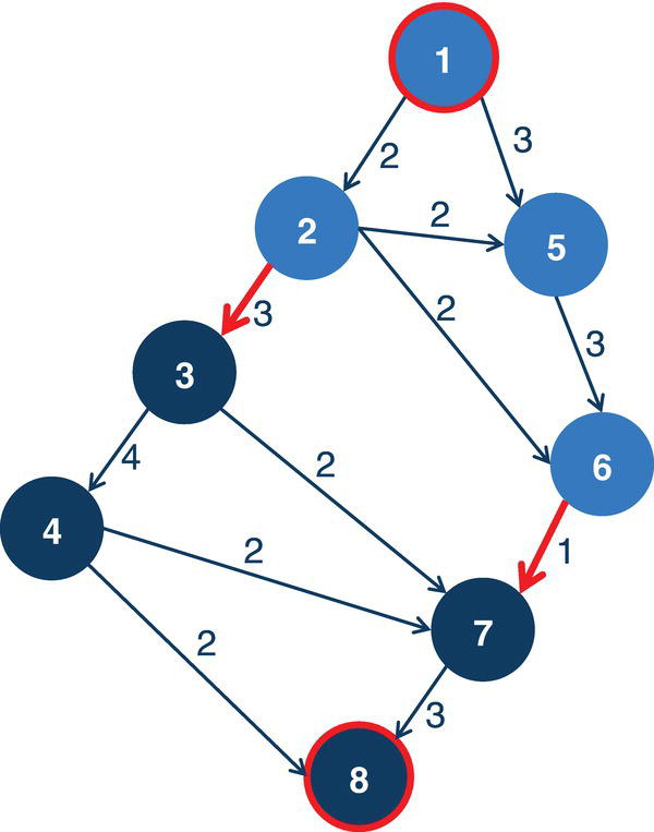
Figure 4.52 Minimum s‐t cut problem.
4.8 Minimum Spanning Tree
The minimum spanning tree problem aims to identify the minimum number of links that connect the entire network. This set of links in the minimum spanning tree keeps the same reachability of the original network, considering all original links within it. A single graph can have many different spanning trees, which may keep the same reachability of the nodes in different ways, by using a different subset of links. The minimum spanning tree problem has many applications in the design of networks. The minimum spanning tree algorithm can be applied in many varied industries like telecommunications, computers, transportation, supply chain, electrical grids, among others.
A minimum spanning tree is a subset of the original set of weighted links within an undirected graph that connects all the nodes together with the minimum possible total link weight.
Given an undirected graph G = (N, L), a spanning tree of the graph G is a tree that spans G and is a subgraph of G. That means, the spanning tree includes every node of G and all the links belonging to G. The cost of the spanning tree is the sum of the weights of all links within the tree. A regular graph can have many spanning trees. The minimum spanning tree is the spanning tree where the cost (the sum of the link weight) is minimum among all the spanning trees within the graph. Of course, it is possible that a graph has multiple minimum spanning trees with it.
When weights are assigned to the links, a minimum spanning tree is a spanning tree where the sum of link weights is less than or equal to the sum of the link weights of every other spanning tree. More generally, any undirected graph has a minimum spanning forest (considering the graph is not connected), which is a union of minimum spanning trees of its connected components.
In proc optnetwork, the MINSPANTREE statement invokes the algorithm that solves the minimum spanning tree problem. The algorithm to solve the minimum spanning tree in proc optnetwork is based on the Kruskal's algorithm. This algorithm can scale to large graphs. Kruskal's algorithm builds the spanning tree by adding links one by one into a growing spanning tree. The algorithm follows a greedy approach as in each iteration it finds the link that has the minimum weight and adds it to the growing spanning tree. A minimum spanning can't have any cycle. Then, the algorithm selects at each iteration the link with the lowest weight and checks if by adding that link to the growing spanning tree a cycle will be created. If not, it keeps searching for the next lowest link weight. If it creates a cycle, it just ignores that link and moves on searching for the next lowest link weight within the graph. In the end, all the links selected, those which avoid any cycles, will be the minimum spanning tree, and will have the cost of the sum of all link weights selected.
There is one single option for the minimum spanning tree algorithm in proc optnetwork. This option specifies the dataset with the final result of the minimum spanning tree problem. The option OUT= defines the output table containing all the resulting links within the minimum spanning tree.
The minimum spanning tree algorithm doesn’t require the nodes dataset. The definition of the links within the graph is crucial for the minimum spanning tree algorithm. It defines the constraints in searching for the minimum weighted links. The links dataset is defined using the LINKS= option. As stated before, the minimum spanning tree algorithm is tailored for undirected graphs. Then, the DIRECTION= option must be specified as directed. In the LINKSVAR statement, the variables from= and to= are used to define the link x ij , the variable weight= is used to receive the link weight. The link weights will be used in searching the optimal solution for the minimum spanning tree problem.
Notice that, like in other algorithms, it is still possible to define the output tables using the options OUTLINKS= and OUTNODES=. However, these options have no effect on the final results and only store the list of nodes and the list of links in the respective output tables.
4.8.1 Finding the Minimum Spanning Tree
Let's consider a simple example to demonstrate the minimum spanning tree problem using proc optnetwork. Consider the graph presented in Figure 4.53. It shows a network with 7 nodes and 11 links. All nodes within the network can reach to each other, even by using multiple steps or links. For example, node A is directly connected to node B. However, node A is not directly connected to node E, but it can reach out to node E passing by nodes B and C. The minimum spanning tree needs to keep the same reachability, making all nodes reach each other by using a set of steps or links between them. The total link weight considering these 11 links is 90. The goal of the minimum spanning tree is to find a subset of the original set of links that keep all nodes connected with a lower total link weight.
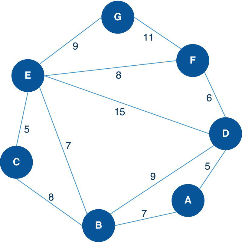
Figure 4.53 Network flow nodes and weighted links.
The following code describes how to create the input dataset for the minimum spanning tree problem. The nodes dataset is not required for the minimum spanning tree algorithm. The links dataset defines the connections between the nodes, and for each connection, the weight for the link, which is used by the algorithm to calculate the minimum link weight when selecting the links to keep the reachability among the nodes.
data mycas.links;input from $ to $ weight @@;datalines;A B 7 A D 5 B C 8 B D 9 B E 7 C E 5D E 15 D F 6 E F 8 E G 9 F G 11;run;
Once the links dataset is created, we can now invoke the minimum spanning tree algorithm using proc optnetwork. The following code describes how to do it. Notice the links definition using the LINKSVAR statements. The variable from, to, and weight receive the links definition. The option DIRECTION= defines the direction of the graph. For the minimum spanning tree problem, the network direction must be undirected.
proc optnetworkdirection = undirectedlinks = mycas.links;linksvarfrom = fromto = toweight = weight;minspantreeout = mycas.outminspantree;run;
Figure 4.54 shows the output for the minimum spanning tree algorithm. It says an optimal solution was found and the objective function is 39. The objective function in the minimum spanning tree problem is the total link weight for the set of links selected as minimum link weighted spanning tree.
Figure 4.55 shows the minimum spanning tree results. The OUTMINSPANTREE dataset shows the original links, which belong to the minimum link weighted spanning tree. Like in other network optimization algorithms, it is still possible to define the output tables using the options OUTLINKS= and OUTNODES=. These options however have no effect the output results. The output table specified in the option OUTLINKS= will be exactly the same as the original links dataset. The output table specified in the option OUTNODES= will have only the list of the nodes.
Notice that the minimum spanning tree has 6 links out of the original 11 links. The total link weight for these 6 links is 39. In other words, the reachability of the original network with 11 links and total link weight of 90 can be maintained by using only 6 links (54% of the original links) with a total link weight of 39 (43% of the original total link weight). In large networks the savings can be substantial when finding the minimum spanning trees.
Figure 4.56 shows the solution for the minimum spanning tree problem, highlighting in the original network the links included in the minimum spanning tree.
The optimal solution defines the links F‐D, D‐A, A‐B, B‐E, C‐E, and E‐G as the minimum spanning tree. These links keep the same reachability among the nodes of the original 11 links, but with a lower total link weight, 39 instead of 90. Notice that some link connections are now a little bit longer, or requiring more steps, or going throughout additional nodes. For example, node G could access node F in a straight connection, with a cost of 11. By using the minimum spanning tree set of links, node G needs to go through nodes E, B, A, and D to reach out to node F. The total cost is now 34, against the original 11. However, the minimum spanning tree requires less links in a much lower total link weight to keep the same nodes’ reachability of the original network.
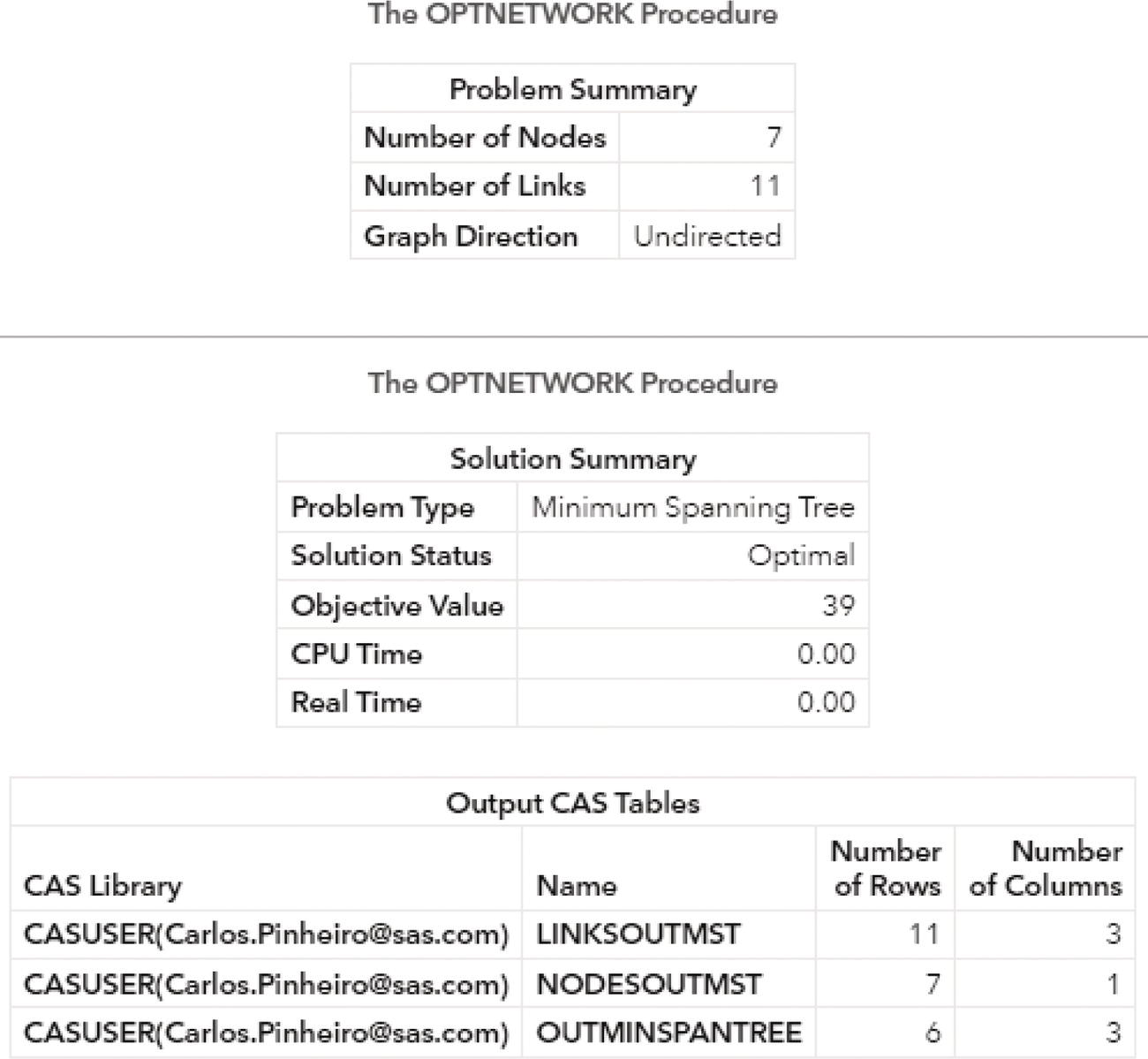
Figure 4.54 Output results by proc optnetwork running the minimum spanning tree algorithm.
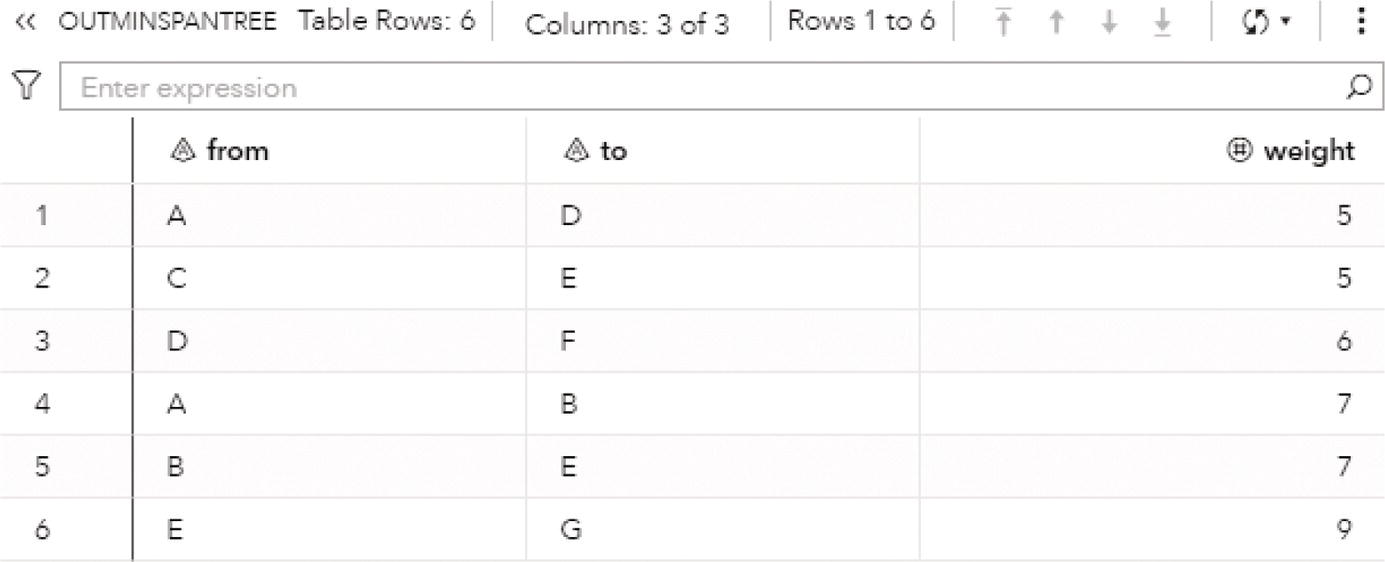
Figure 4.55 The minimum spanning tree solution.
4.9 Path
In graph theory, a path in a graph G = (L, N) is an ordered sequence of links (l 1, l 2, l 3, …, l n − 1), which connects an ordered sequence of nodes (n 1, n 2, n 3, …, n n ). In a path, all nodes n i , where 1 ≤ i ≤ n, belong to the set of nodes N. For two consecutive nodes there is a link l ij that belongs to the set of links L. A simple path is a path where all nodes n 1, …, n n .are distinct. No node appears more than once in the sequence. The sequence of links is ordered in a way where the destination node of each link is the origin node of the next link. In a simple path, no node is visited more than once. A simple path has no cycles. A path between any two nodes i and j in a graph is a path that starts at i and ends at j. The starting node is called the source node, and the ending node is called the sink node. A path can be computed in both directed and undirected graphs. In undirected graphs, a duplicate link is created to represent both directions. For example, a link between nodes A and B are represented by 2 links A‐B and B‐A.
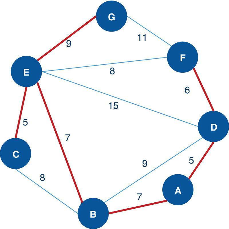
Figure 4.56 Minimum spanning tree results.
Paths are fundamental concepts in graph theory. They have many applications in graphs describing communications network, power distribution, transportation, and computer networks, among many others.
In proc optnetwork, the PATH statement invokes the algorithm that solves the path enumeration problem, which finds the elementary or simple paths of an input graph. Proc optnetwork finds by default all elementary paths for all pairs of nodes in the input graph. That means, the algorithm finds all paths for all possible combinations of source and sink nodes. Finding all paths possible in an input graph means not just time consuming but possibly a huge output. Even for a small network, with only a few nodes and links, the algorithm for the path enumeration can produce an output with hundreds of possible paths. An alternative method to reduce the output is to find paths in an input graph by limiting the number of source and sink nodes. The algorithm will search for all simple paths just between these sets of nodes, starting from the set of nodes defined as source nodes, and ending with the set of nodes defined as sink nodes.
There are many options for the path enumeration algorithm in proc optnetwork. Something very important in all the input graphs we have been analyzing is the weight or the cost of each link. The link weight doesn't affect the path enumeration directly, or the way the algorithm finds all the simple paths among all the nodes, but it affects the way the algorithm evaluates the paths’ total link weight. The option WEIGHT= in the LINKSVAR statement can be used to specify the weight of the links in the weighted graphs. Alternatively, there is an option AUXWEIGHT= which can also be used to specify an auxiliary weight for the links in the input graph. Eventually the link weight may be the inverse of the original weight to lead the algorithm in maximizing or minimizing an objective function, or the original link weight can be weighted in a different way to represent a particular business scenario. Finally, the direction of the link can be both directed and undirected. If we create the links dataset considering the direction of the link, the from node will be the source node and the to node will be the sink node. That link will be unique. Based on the same links dataset, we can also define an undirected graph, and then, each link will be duplicated and both directions will be evaluated by the algorithm. For example, a path A → B → C in a directed graph becomes two paths A → B → C and C → B → A in an undirected graph.
The final result for the path enumeration algorithm in proc optnetwork is reported and saved in output tables defined by the OUTPATHSLINKS= and OUTPATHSNODES= options. The output table specified in the OUTPATHSLINKS= option saves all the links comprised in all the paths, considering all possible pairs of source‐sink nodes. The option OUTPATHS= has the same effect and can be used in place of the option OUTPATHSLINKS=. If there is no source‐sink pair defined by the options SOURCE= and SINK=, or no source‐sink pairs are defined using the option NODESSUBSET=, all nodes are used to create the combinations of source and sink nodes. This may create a huge output data table as a result, particularly for large networks. The output data table specified using the OUTPATHSNODES= option saves all the nodes comprised in all of the paths, considering again all possible pairs of source‐sink nodes. Analogously, if no source‐sink pair is defined, all nodes within the network are selected to create the source‐sink pairs of nodes. As the output tables produced by the path enumeration algorithm can be extremely large, depending on the size of the network and/or the number of source‐sink pairs of nodes defined, the time to generate these output tables can be longer than the time to compute the paths.
The output table specified in the OUTPATHSLINKS= option contains all the links in each path, including the columns to describe them. The variable source contains the label of the source node of the path. The variable sink contains the label of the sink node of the path. The variable path identifies a particular source‐sink pair of nodes, which is the path identification. The variable order identifies the order of the link within the path for that particular source‐sink pair of nodes, which ultimately is the order of the link in the path identified by the variable path. The variable used in the from= option in the LINKSVAR statement identifies the label of the from node of the link within the path. The variable used in the to= option in the LINKSVAR statement identifies the label of the to node of the link within the path. The variable used in the weight= option in the LINKSVAR statement identifies the weight of the link within the path. Finally, the variable used in the auxweight= option in the LINKSVAR statement identifies the auxiliary weight of the link within the path. For example, if we define in the links dataset the variables org, dst, wgt, and auxwgt to define the from node, the to node, the link weight, and the auxiliary link weight, respectively, the output table will contain all these variables in addition to the output variables source, sink, path, and order.
The output table specified in the OUTPATHSNODES= option contains all the nodes within each path. This output table contains the following columns. The variable source identifies the label of the source node of the path. The variable sink identifies the label of the sink node of the path. The variable path identifies the source‐sink pair, which ultimately defines the path identifier. The variable order identifies the order of the source‐sink pair within the path. The variable used in the node= option in the NODESVAR statement identifies the label of the node within the path. The variable used in the weight= option in the NODESVAR statement identifies the weight of the node within the path. For example, if we define in the nodes dataset the variables n and wgt to represent the label of the node, and the weight of this node within the network, respectively, the output table will contain all these variables in addition to the original output variables source, sink, path, and order.
Therefore, we can define both input network elements to proc optnetwork, which means the links and nodes datasets. The links dataset is specified by using the option links=, and the nodes dataset is specified by using the option nodes=. The links and nodes datasets specify the input graph considered by proc optnetwork when computing the paths. The definitions of both links and nodes datasets are particularly important when the weight for both links and nodes are required to describe a particular business scenario. For example, important relations between entities within the network and important entities within the network. In banking, we can assume relations as transactions between accounts. Then, the amount transferred between these accounts is quite relevant and it will be represented by the link weight. Similarly, the account balance is important to identify relevant entities, and then it will be represented by the node weight.
By default, proc optnetwork computes all possible paths within the input graph, considering all possible combinations of source and sink nodes. The list of nodes is combined by pairs and then, all possible paths between these pairs of source and sink nodes are searched by the path enumeration algorithm. As we saw before, the final result can be exhaustive. The output tables can be extremely large. In order to prevent proc optnetwork from generating large final outcomes, we can alternatively use the options SOURCE= and SINK= to specify the source nodes, the sink nodes, or the pairs of source and sink nodes where the paths will be searched. These options work independently. For example, to fix a particular source node and find all paths departing from the fixed source node to all possible sink nodes within the input graph, we use the SOURCE= option. Analogously, to fix a particular sink node and find all paths from all possible source nodes arriving at the fixed sink node, we use the SINK= option. By using both SOURCE= and SINK= options, we fix a particular source node and a particular sink node. By doing that, proc optnetwork will search for all paths between the fixed source node to the fixed sink node, the paths departing from the fixed source node and arriving at the fixed sink node.
An alternative way is by using a subset of nodes. The options SOURCE= and SINK= define a single source node and/or a single sink node. The option NODESSUBSET= specifies a dataset containing a list of nodes and a definition if the node will be used as a source node and/or as a sink node. The NODESSUBSETVAR statement specifies a variable node as the node identification, a variable source that indicates if the node will be used as a source node, and a variable sink that indicates if the node will be used as a sink node. The concept of a subset of nodes within the input graph applies to the path and shortest path algorithms.
It is important to notice that the settings for the options SOURCE= and SINK override the use of the variable source and sink specified in the NODESSUBSET= option when proc optnetwork searches for the paths within an input graph.
In addition to the SOURCE= and SINK= option, there are other options that reduce the size of the final output table produced by proc optnetwork when running the path enumeration algorithm.
The option MAXLENGTH= specifies the maximum number of links contained in a path. Any path that has the number of links greater than the number specified in the option is removed from the results. The default is the largest number that can be represented by a 32‐bit integer, which basically means all possible lengths. When the default is used, no paths are removed from the results. Depending on the problem, it is always a good idea to limit the length of the paths returned as a result of the path enumeration algorithm. These shorter paths may have more business meaning depending on the problem or the business scenario.
In reverse, the option MINLENGTH= specifies the minimum number of links contained in a path. Any path that has fewer links than the number specified in the option is removed from the results. By default, the value for the option MINLENGTH= equals to 1. By using the default value, no paths are removed from the results.
The option MAXLINKWEIGHT= specifies the maximum sum of link weights contained in a path. Any path that has the sum of link weights greater than the number specified in the option is removed from the results. Again, the default value is the largest number that can be represented by a double, which basically means, any possible sum of link weights. When the default is used, no paths are removed from the results. Analogously to the maximum length of the path, the maximum sum of link weights can reduce the size of the output table to more meaningful paths according to the problem or the business scenario under analysis.
The other option, MINLINKWEIGHT= specifies the minimum sum of link weights contained in a path. Any path that has the sum of link weights less than the number specified in the option is removed from the results. The default is the largest (in magnitude) negative number that can be represented by a double. That basically means any link weights in the negative value. When the default is used, no paths are removed from the results.
The option MAXNODEWEIGHT= specifies the maximum sum of node weights contained in a path. Any path that has the sum of node weights greater than the number specified in the option is removed from the results. The default is the largest number that can be represented by a double. When the default is used, no paths are removed from the results. Reducing the number of paths returned by the path enumeration based on a particular maximum node weight cannot just reduce the path range to analyze but can highlight more meaningful paths according to a particular problem or business scenario.
In reverse to the maximum node weights, the option MINNODEWEIGHT= specifies the minimum sum of node weights contained in a path. Any path that has the sum of node weights less than the number specified in the option is removed from the results. The default is the largest (in magnitude) negative number that can be represented by a double. The default value basically means any negative number, which causes no paths to be removed from the results.
Another option to reduce the number of paths to be reported in the output table is to limit the time of running. The option MAXTIME= specifies the maximum amount of time that proc optnetwork will spend searching for the possible paths. The type of time (either CPU time or real‐time) is determined by the value defined in the TIMETYPE= option. The default is the largest number that can be represented by a double. Limiting the running time is also a good approach to reduce the number of paths to be analyzed according to the problem or business scenario.
4.9.1 Finding Paths
Let's consider a simple graph to demonstrate the path enumeration problem using proc optnetwork. Consider the graph presented in Figure 4.57. It shows a network with just 6 nodes and only 11 links. It is important to emphasize here that even with a very small network, the number of paths found in the path enumeration problem can be large. As the input graph grows larger, the process can be exhaustive, and the output table can be extremely large or even unfeasible.
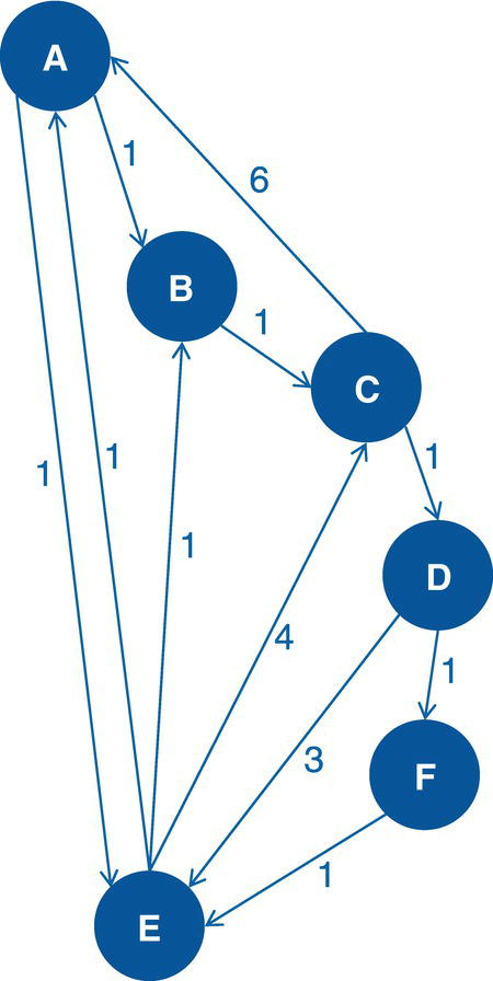
Figure 4.57 Directed input graph with weighted links.
The following code describes how to create the input dataset for the path enumeration problem. At first, only the links dataset will be defined. Later on, we will see the impact of defining both links and nodes datasets to represent the input graph. The links dataset has the nodes identification, the from and to variables, and the weight of the link. This dataset can be used to represent both directed and undirected graphs as we will see in the following examples.
data mycas.links;input from $ to $ weight @@;datalines;A B 1 A E 1 B C 1 C D 1 C A 6 D E 3D F 1 E A 1 E B 1 E C 4 F E 1;run;
Once the input dataset is defined, we can now invoke the path enumeration algorithm using proc optnetwork. The following code describes how to do it. Notice the links definition using the LINKSVAR statements. For the links, the variable weight receives the weight of the link, and the variables from and to receive the source and the sink nodes. As there is no SOURCE= or SINK= option being used, all possible pairs of nodes combinations will be used as sources and sinks nodes within this input graph. The input graph in this example is defined as a directed network.
proc optnetworkdirection = directedlinks = mycas.links;linksvarfrom = fromto = toweight = weight;pathoutpathslinks = mycas.outpathlinksoutpathsnodes = mycas.outpathnodes;run;
Figure 4.58 shows the output for the path enumeration algorithm. It says an optimal solution was found (solution status is ok) and the number of paths found between all possible pairs of nodes is 86.
The following pictures show the path enumeration results. The OUTPATHLINKS dataset presented in Figure 4.59 shows the original variables, the from and to which defines the source and the sink nodes in the link, and the variable weight, which defines the weight of this link. In addition to that, the output table shows the variables source and sink, which defines from where the path departs and to where it arrives. Finally, the output table also shows the variables path, which is the path identifier, and the variable order, which identifies the order of link within that particular path.
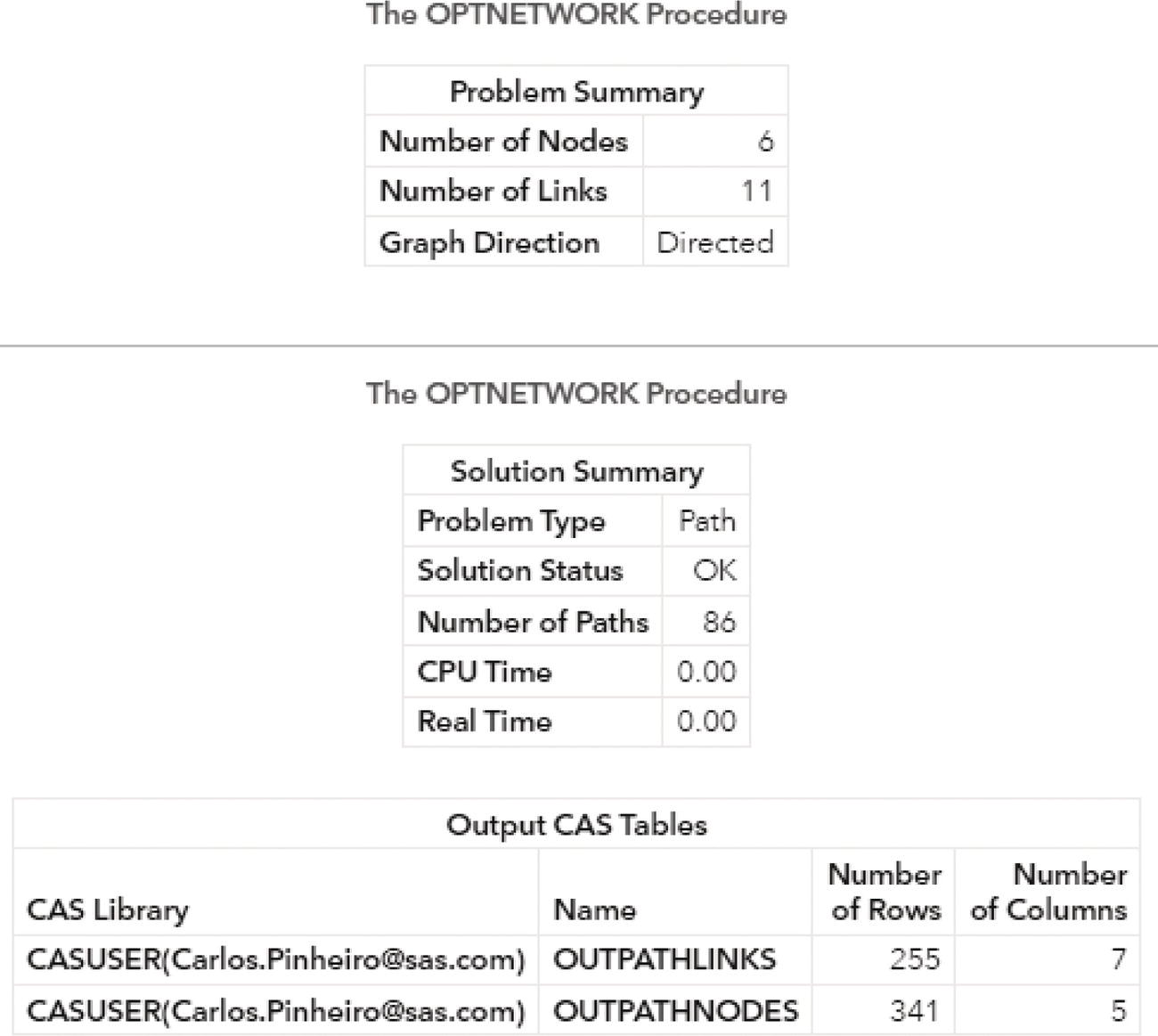
Figure 4.58 Output results by proc optnetwork running the path enumeration algorithm on a directed input graph.
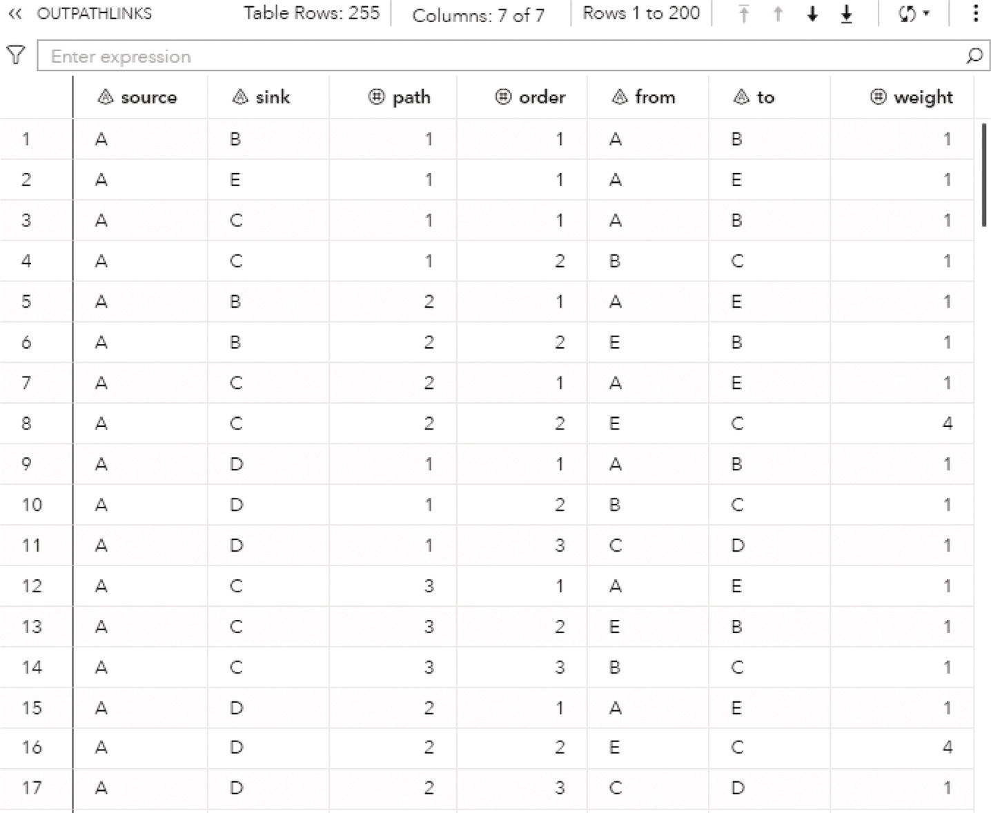
Figure 4.59 The path enumeration solution for the links.
For example, line 1 describes a path comprising one single link. The source node is A, the sink node B, and the path has a unique link from A to B. Lines 3 and 4 describe a bit longer path. The source node is A again, the sink node is C, but this path has 2 links, from A to B and then from B to C. As we can see on the top of the picture, this output table has 255 rows, describing all 86 paths found by the path enumeration algorithm. This picture shows only the first 17 rows.
Proc optnetwork also produces an output for the nodes. The OUTPATHNODES dataset presented in Figure 4.60 shows the variables source to identify the source node of the path, the variable sink to identify the sink node of the path, the variable path to identify the path, the variable order to identify the order of the link within the path and the variable node to identify the node within that particular link/path.
Notice that the variable order describes the sequence of the links where the node is. For example, lines 1 and 2 describes the path from the source node A to the sink node B. Line 1 describes node A in order 1, and line 2 describes node B in order 2. In other words, this path goes from node A to node B. Lines 5, 6, and 7 describes a longer path. The source node is A, and the sink node is C. Line 5 describes node A in order 1, line 6 describes node B in order 2, and finally line 7 describes node C in order 3. This path goes from node A to B and then from B to C. This path has 2 links.
Let's take a look at the use of the options SOURCE= and SINK= to reduce the number of paths searched by the path enumeration algorithm in proc optnetwork. The next example describes the option SOURCE= to fix a particular node when searching the paths within the input graph. All paths returned by the path enumeration algorithm need to start at the node specified in the option SOURCE=. All other nodes can be the sink node. The following code show how to fix a source node when searching for the paths:
proc optnetworkdirection = directedlinks = mycas.links;pathsource = 'A'outpathslinks = mycas.outpathlinksoutpathsnodes = mycas.outpathnodes;run;
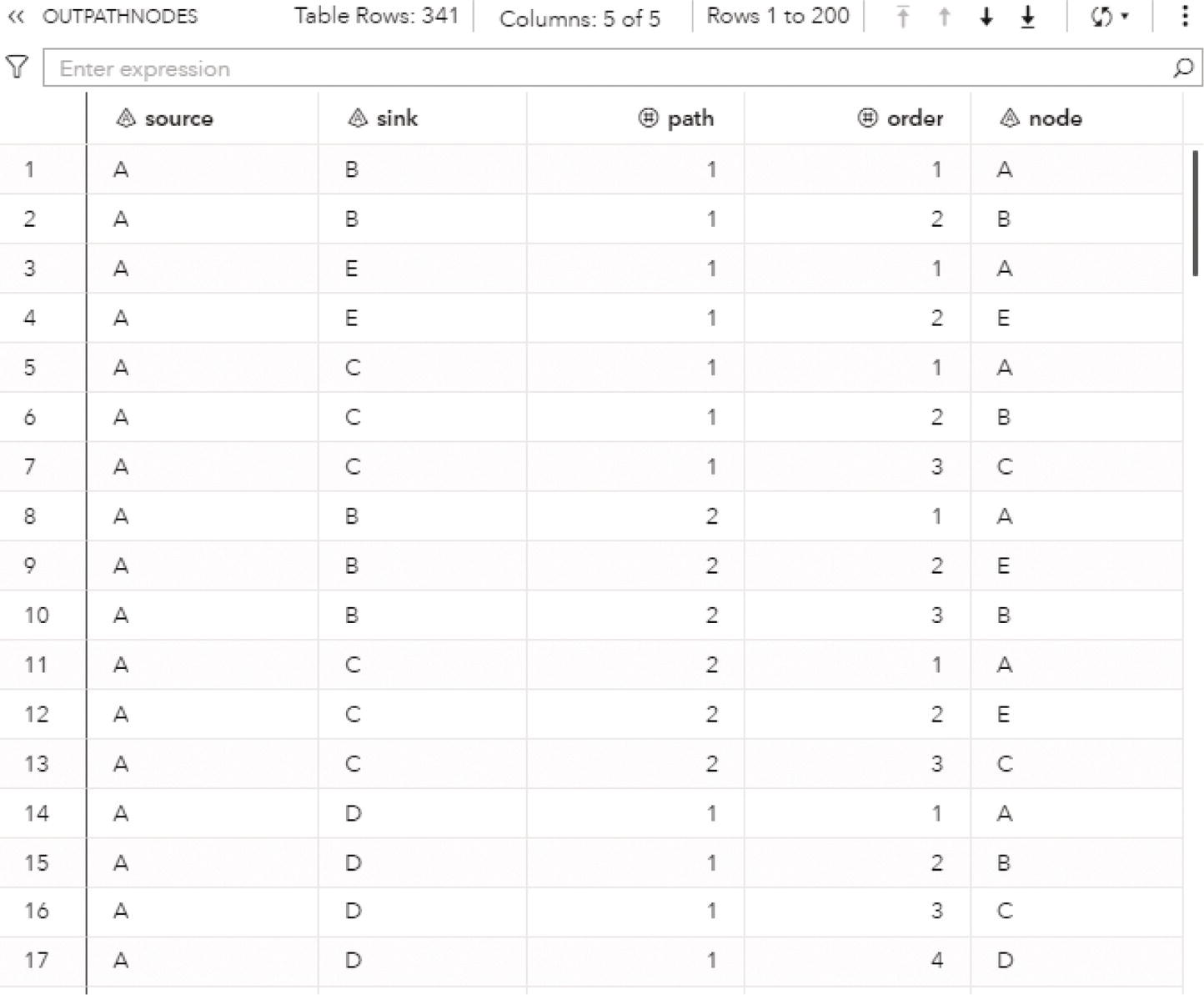
Figure 4.60 The path enumeration solution for the nodes.
Figure 4.61 shows the output produced by proc optnetwork. Notice that only 14 paths were found when the source node is fixed as node A.
Figure 4.62 shows the result table for the path enumeration algorithm. Notice that the source node for all rows is node A. This output table shows then all paths starting at the source node A and ending at any possible sink node within the input graph.
The output table OUTPATHLINKS contains all 43 links comprised by the 14 paths starting at the source node A.
Analogously, we can define only a sink node when executing the path enumeration algorithm in proc optnetwork. The following code shows how to define a sink node to search for all paths ending at a fixed sink node.
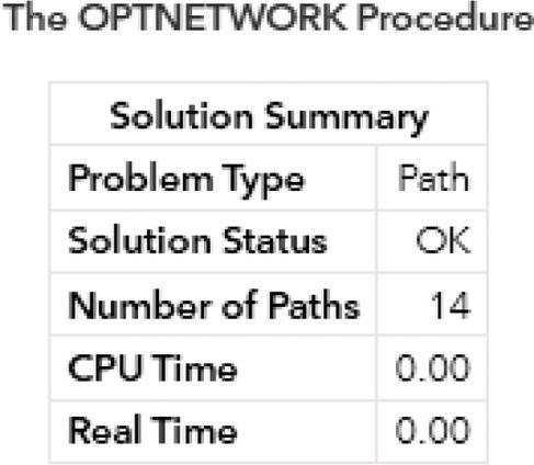
Figure 4.61 The path enumeration solution with a fixed source node.
proc optnetworkdirection = directedlinks = mycas.links;pathsink = 'D'outpathslinks = mycas.outpathlinksoutpathsnodes = mycas.outpathnodes;run;
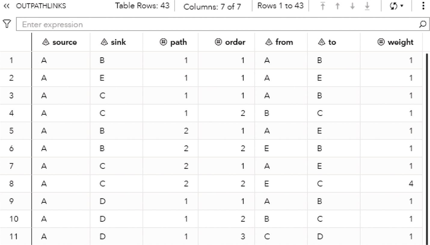
Figure 4.62 The path enumeration solution for the links using a fixed source node.
Figure 4.63 shows the output produced by proc optnetwork. Notice that only 11 paths were found when the sink node is fixed as node D.
Figure 4.64 shows the result table for the path enumeration algorithm. Notice that the sink node for all rows is node D. This output table then shows all paths starting at any possible node within the input graph and ending at the sink node D.
The output table OUTPATHLINKS contains all 34 links comprised by the 11 paths ending at the sink node D.
Finally let's take a look at an example where both source and sink nodes are fixed. Proc optnetwork will search for all possible paths within the input graph where the source node is the node fixed by the option SOURCE= and the sink node is the node fixed by the option SINK=. The following code shows how to fix both source and sink nodes.
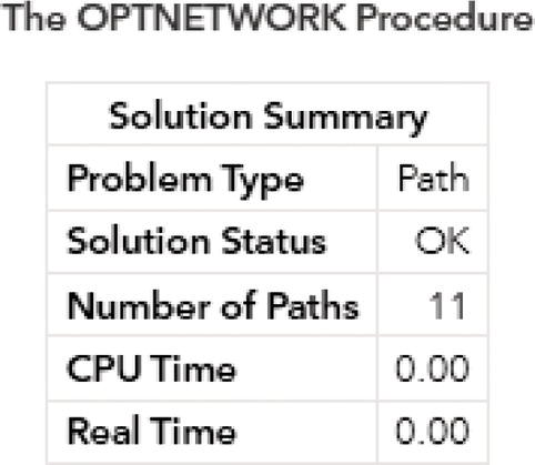
Figure 4.63 The path enumeration solution with a fixed sink node.
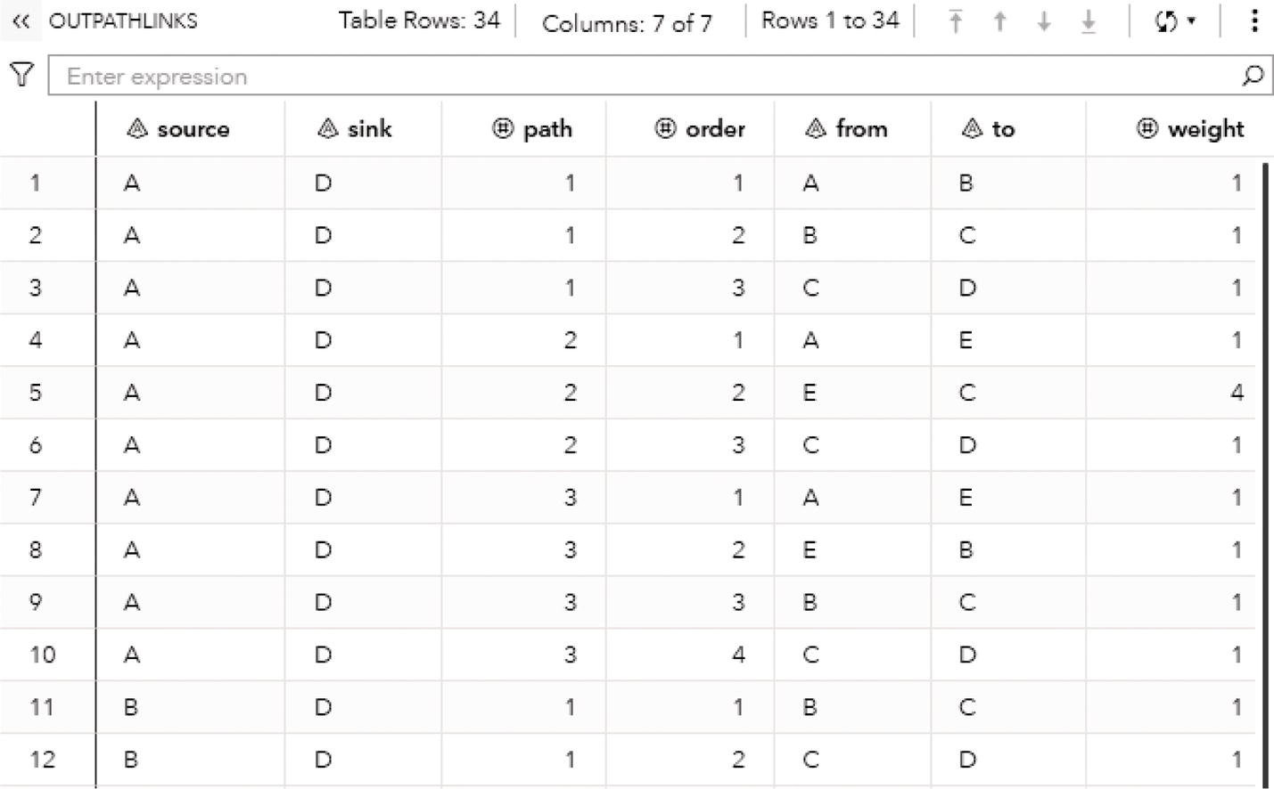
Figure 4.64 The path enumeration solution for the links using a fixed sink node.
proc optnetworkdirection = directedlinks = mycas.links;pathsource = 'A'sink = 'D'outpathslinks = mycas.outpathlinksoutpathsnodes = mycas.outpathnodes;run;
Figure 4.65 shows the output produced by proc optnetwork when running the path enumeration algorithm for fixed source and sink nodes. Notice that only 3 paths were found when the source node is fixed as node A and the sink node is fixed as node D.
Figure 4.66 shows the result table for the path enumeration algorithm. Notice that the source node for all rows is node A and the sink node for all rows is node D. This output table then shows all paths within the input graph starting at node A and ending at node D.
The output table OUTPATHLINKS contains all 10 links comprised by the 3 paths starting at node A and ending at the sink node D.
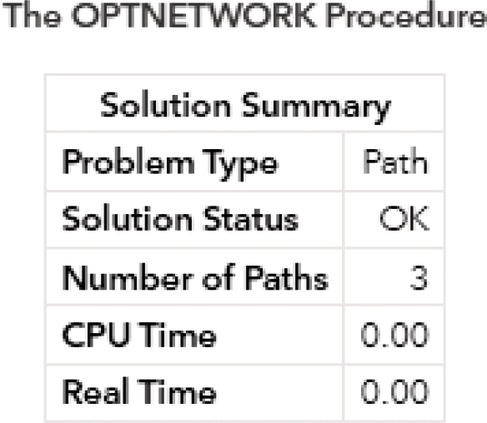
Figure 4.65 The path enumeration solution for fixed source and sink nodes.
Figure 4.67 shows the original input graph highlighting the source node A and the sink node D.
Figure 4.68 shows the solution for the path enumeration algorithm considering the input graph with the source node fixed as node A and the sink node fixed as node D.
Notice that there are only 3 paths starting from node A and ending to node D, A → B → C → D, A → E → C → D and A → E → B → C → D.
Lastly, let’s take a look at the path enumeration algorithm for an undirected graph. Also, let's use different column names for the original nodes and links datasets in order to show how proc optnetwork produces the final output tables.
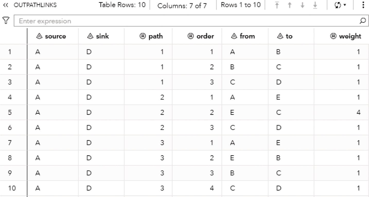
Figure 4.66 The path enumeration solution for the links using fixed source and sink nodes.
The following code describes how to create the input datasets for the path enumeration problem. In this example we are using both links and nodes datasets. For the links dataset we have the variable a to represent the from node, the variable b to represent the to node, the variable wgt to represent the weight of the link, and the variable aux to represent the auxiliary weight for the link. As an undirected graph, the from node doesn't necessarily represent the source node in the path enumeration problem. The same concept applies to the to node. It doesn't necessarily represent the sink node. For an undirected graph, proc optnetwork duplicates the links under the hood to compute all possible paths considering both directions. For example, the following datasets create a link starting at node A and ending at node B. As an undirected graph, we can also have a link staring at node B and ending at node A. Proc optnetwork creates this second link internally in order to compute the path enumeration for an undirected input graph.
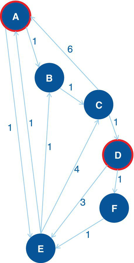
Figure 4.67 Input graph with fixed source and sink nodes.
data mycas.links;input a $ b $ wgt aux @@;datalines;A B 1 0.5 A E 1 0.5 B C 1 0.5 C D 1 0.5 C A 6 0.17 D E 3 0.33D F 1 0.5 E A 1 0.5 E B 1 0.5 E C 4 0.25 F E 1 0.5;run;
Here we also create a nodes dataset to show how proc optnetwork produces the final output tables. This nodes dataset has the variable n to define the node and the variable wgt to define the weight of the node.
data mycas.nodes;input n $ wgt @@;datalines;A 10 B 15 C 5 D 20 E 25 F 30;run;
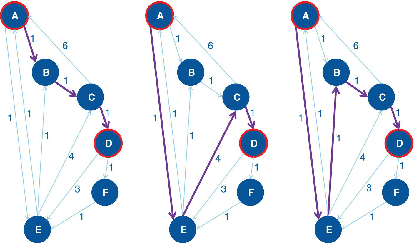
Figure 4.68 The path enumeration solution for the nodes.
The following code describes how we specify the nodes and links variables when solving the path enumeration problem with proc optnetwork. The DIRECTION= option defines the input graph as undirected. The LINKSVAR and NODESVAR statements define the links and nodes properties, respectively by using the variables from, to, weight and auxweight for the links, and the variables node and weight for the nodes.
proc optnetworkdirection = undirectedlinks = mycas.linksnodes = mycas.nodes;linksvarfrom = ato = bweight = wgtauxweight = aux;nodesvarnode = nweight = wgt;pathoutpathslinks = mycas.outpathlinksoutpathsnodes = mycas.outpathnodes;run;
Figure 4.69 shows the output for the path enumeration algorithm when running on an undirected input graph. An optimal solution was achieved, and the number of paths found between all possible pairs of nodes is 422. Recall that for the same number of links on a directed input graph, the path enumeration found 86 paths. The major difference is the number of internal links on the input graph. For the directed graph, the 11 links remain as 11 links respecting the from and to nodes (source and sink nodes). For the undirected graph, the 11 links are internally duplicated creating 22 links for both directions between the from and to nodes. That duplication creates more possible combinations of source and sink pairs of nodes for the input graph, and then, more paths found by the algorithm, 422 against 86. Notice that the output states 6 nodes and 11 links. These are the original 11 links in the links dataset. But as an undirected graph, proc optnetwork treats each link as having actually 2 directions.
The following pictures show the path enumeration results. The OUTPATHLINKS dataset presented in Figure 4.70 shows the original variables a and b, which defines the origin and the destination nodes for each link, the variable wgt, which defines the weight of the link, and the variable aux, which defines the auxiliary weight for the link. Additionally, the output table has the variables source and sink, which defines the origin and the destination nodes for the path. Finally, the output table also shows the variables path, which is the path identifier, and the variable order, which identifies the order of links within that particular path.
The concept is similar to the one presented before for the directed graph. A small difference should be noticed here. For example, line 2 shows a path A‐C, with a unique link C‐A. At line 544, we can see a path C‐A with the same link C‐A. The path C‐A is natural, associated with the unique link C‐A. But what explains the path A‐C with a link C‐A? This happens because of the nature of the undirected graph. Internally, proc optnetwork “duplicates” the link C‐A, creating an imaginary link A‐C. That makes a path A‐C possible with the original link C‐A (the “duplicated link A‐C). The same thing happens on lines 3 and 4. We can see the same path A‐E with unique links E‐A and A‐E, respectively. This happens because in the links dataset we actually have both links A‐E and E‐A. Then, we will observe 4 paths, 2 paths A‐E with unique links E‐A and A‐E (lines 3 and 4), and 2 paths E‐A with unique links E‐A and A‐E again (lines 1013 and 1014).
The OUTPATHNODES dataset presented In Figure 4.71 will be similar to the one presented for the directed graph, but with many more rows in order to describe all the paths found. This output table has 1872 rows against 341 rows for the directed graph. The output table presents the variables source and sink to identify the source and sink nodes of the path, the variable path to identify the path, the variable order to identify the order of the link within the path, and the original variables created in the nodes dataset, n to identify the node and wgt to identify the weight of the node.

Figure 4.69 Output results by proc optnetwork running the path enumeration algorithm on an undirected input graph.
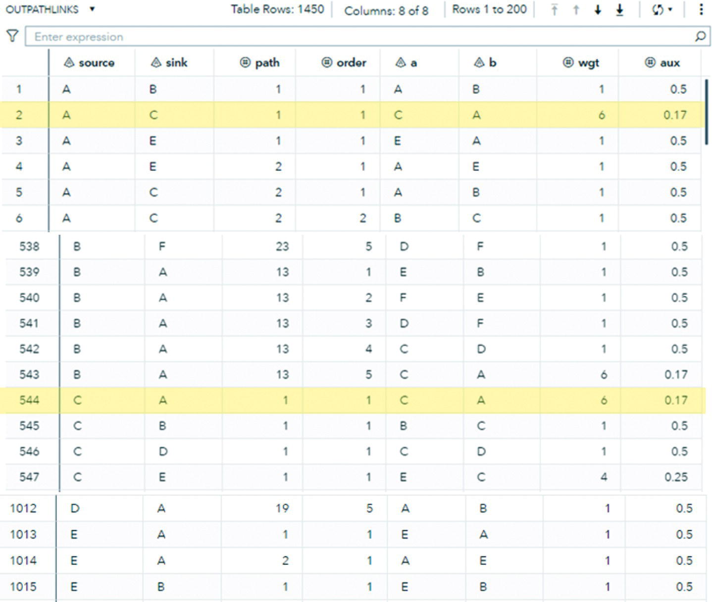
Figure 4.70 The path enumeration solution for the links.
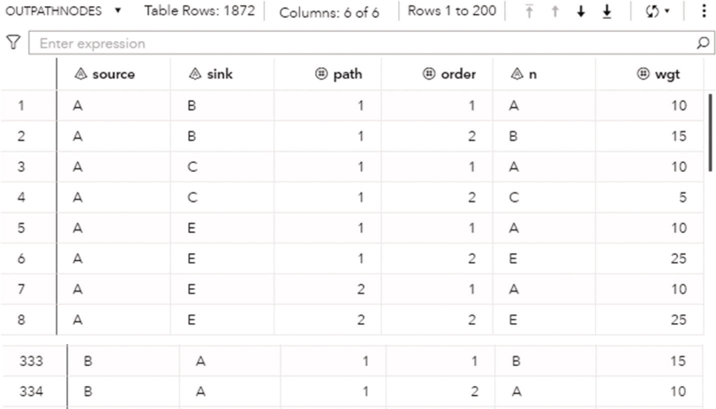
Figure 4.71 The path enumeration solution for the nodes.
Analogously to the links output, the output table for the nodes presents the duplications appearance for the nodes. Node A appears in the path A‐B shown in line 1 as well as in path B‐A shown in line 334. The same for node B, it appears in path A‐B showed in line 2 and in path B‐A shown in line 333. This happens even though there is only the link A‐B defined in the links dataset. Proc optnetwork “duplicates” that link to create an imaginary link B‐A to represent the undirected graph.
4.10 Shortest Path
As we saw in the previous section, a path in an input graph is an ordered sequence of links which connects an ordered sequence of nodes. All nodes in a path are distinct. No node appears more than once in the sequence.
The shortest path problem is aimed to find the path between two nodes in an input graph where the sum of the weights of its links is minimized. There is a set of real‐life problems that can be addressed by the shortest path, such as road networks, public transportation planning, traffic planning, sequence of choices in decision making, minimum delay in telecommunications, operations research, layout facility, and robotics, among many others.
Formally, the shortest path between two nodes i and j in an input graph is the path that starts at node i and ends at node j with the lowest total link weight. Like in the path enumeration problem, the starting node is referred to as the source node and the ending node is referred to as the sink node.
By default, proc optnetwork computes the shortest paths for all pairs of nodes within the network. Similarly to the path algorithm, that means to find the shortest path between all possible combinations of source nodes and sink nodes within the input graph. This outcome can result in an extremely large output table. To reduce the size of the outcome, alternatively we can select the pair of source and sink nodes to search the shortest path or select a subset of nodes to be fixed as source nodes and sink nodes.
In proc optnetwork, the SHORTESTPATH statement invokes the algorithm that solves the shortest path problem. Proc optnetwork uses multiple algorithms to find the shortest path between a pair of nodes. The algorithm used by proc optnetwork when searching for the shortest paths relies on the type of data that describes the input graph. If the graph is unweighted, which means the variable weight is not used to differentiate the importance or the cost of the links within the network, the algorithm that proc optnetwork uses is based on the breadth‐first search. If the graph is weighted, and there is no negative weight to represent the importance or the cost of the links within the network, the algorithm that proc optnetwork uses is based on Dijkstra's algorithm. Finally, if the graph is weighted and there are positive and negative weights to represent the importance or the cost of the links within the network, the algorithm that proc optnetwork uses is based on the Bellman = Ford algorithm.
There are many options for the shortest path algorithm in proc optnetwork. As we saw before, the type of the input graph is relevant to define which algorithm proc optnetwork will use in searching for the shortest paths. The relevancy is if the graph is weighted or unweighted, and if there are positive and negative weights associated with the links within the network. For weighted graphs, proc optnetwork uses the variable weight defined in the links dataset to evaluate all possible paths based on the total link weight, or the total cost of the path. The option WEIGHT= in the LINKSVAR statement is then used to specify the weight of the links in weighted graphs. Alternatively, there is an option AUXWEIGHT=, which can also be used to specify an auxiliary weight for the links within the input graph. The auxiliary weight is not used in the algorithm to calculate the total cost of the path and compare it to the other possible paths when searching the shortest paths. The auxiliary weight is used to calculate a different total cost for each path, and it is reported in the output tables. The auxiliary link weight may be the inverse of the original weight to lead the algorithm in maximizing or minimizing an objective function, or the original link weight can be weighted in a different way to represent a particular business scenario. For example, if we are looking at the total cost of a path, the shortest path between a pair of nodes is the smallest total link weight between the source and sink nodes. In transportation, the shortest path would be the smallest total distance, or the smallest total time, or the smallest total cost (tolls in highways). In social network, we are primarily looking for strong relationships. The shortest path between a pair of nodes in a social scenario would be the path with the highest weight between the source node and the sink node, either based on total frequency or total time. One straightforward way to compute the shortest path in this particular case is to invert the original link weight between the nodes and assign it to the variable weight in the LINKSVAR statement. By doing this, the higher the original weight, the lower the inverse weight, which will contribute most to the shortest path. The original weight will be kept and assigned to the variable auxweight in the LINKSVAR statement. Both original and inverse weights will be included in the final output table.
Similar to the path enumeration problem, the direction for the links in the input graph for the shortest path algorithm can be both directed and undirected. In a particular links dataset, considering a directed graph, the from node will be the source node and the to node will be the sink node when the algorithm searches for the shortest path. Each link in the links dataset is unique. Based on the exact same links dataset, but defining the network as an undirected graph, each link is internally “duplicated” to account for both directions. A defined link (A,B) in the links dataset will represent the link A → B on a directed graph and two links A → B and B → A in an undirected graph.
The final result for the shortest path algorithm in proc optnetwork is reported to the output tables defined by the OUTPATHSLINKS=, OUTPATHSNODES=, OUTWEIGHTS=, and OUTSUMMARY= options. The output table specified in the OUTPATHSLINKS= option saves the links comprised in the shortest paths, considering all possible pairs of source‐sink nodes. If there is no source‐sink pair defined by the options SOURCE= and SINK=, or no source‐sink pairs are defined using the option NODESSUBSET=, all nodes are used to create the combinations of source and sink nodes. This may create a huge output data table as a result, particularly for large networks. The output data table specified using the OUTPATHSNODES= option saves the nodes comprised in the shortest paths, considering again all possible pairs of source‐sink nodes. Analogously, if no source‐sink pair is defined, all nodes within the network are selected to create the source‐sink pairs of nodes. Similar to the path enumeration algorithm, as the output tables produced by the shortest path algorithm can be extremely large, depending on the size of the network and/or the number of source‐sink pairs of nodes defined. Therefore, the time to generate the output tables can be longer than the time to search for the shortest paths.
The output table specified in the OUTPATHSLINKS= option (OUT= and OUTPATHS= options are used alternatively) contains all the links in each shortest path, including the columns to describe them. The variable source contains the label of the source node of the shortest path. The variable sink contains the label of the sink node of the shortest path. The variable order identifies the order of the link within the shortest path assigned to that particular source‐sink pair of nodes. The variable used in the from= option in the LINKSVAR statement identifies the label of the from node of the link within the shortest path. The variable used in the to= option in the LINKSVAR statement identifies the label of the to node of the link within the shortest path. The variable used in the weight= option in the LINKSVAR statement identifies the weight of the link within the shortest path. Finally, the variable used in the auxweight= option in the LINKSVAR statement identifies the auxiliary weight of the link within the shortest path. For example, if we define in the links dataset the variables org, dst, wgt, and auxwgt to define the from node, the to node, the link weight, and the auxiliary link weight, respectively, the output table will contain all these original variables in addition to the output variables source, sink, and order. If we define the maximum number of ranked paths to find for each source‐sink pair by using the option MAXPATHSPERPAIR=, a variable rank will be added to the output table to specify the rank of the link within the shortest path.
The output table specified in the OUTPATHSNODES= option contains all the nodes assigned to each shortest path. This output table contains the following columns. The variable source identifies the label of the source node of the shortest path. The variable sink identifies the label of the sink node of the shortest path. The variable order identifies the order of the source‐sink pair within the shortest path. The variable used in the node= option in the NODESVAR statement identifies the label of the node within the shortest path. For example, if we define in the nodes dataset the variables n to represent the label of the node, the output table will contain that original variable in addition to the output variables source, sink, and order. If we define the maximum number of ranked paths to find for each source‐sink pair by using the option MAXPATHSPERPAIR=, a variable rank will be added to the output table to specify the rank of the source‐sink pair within the shortest path.
The output table specified in the OUTSUMMARY= option contains the summary statistics for the shortest paths for each source node. This output table contains the following variables. The variable source identifies the source node label within the shortest path. The variable paths identifies the number of shortest paths from the source node to the requested sink nodes within the shortest paths. The variable path_weight_min identifies the minimum weight of shortest paths from the source node to all the sink nodes. The variable path_weight_max identifies the maximum weight of shortest paths from the source node to all the sink nodes. The variable path_weight_avg identifies the average weight of shortest paths from the source node to all the sink nodes. The variable path_weight_std identifies the standard deviation of weight of shortest paths from the source node to all the sink nodes. The variable path_weight_var identifies the variance of weight of shortest paths from the source node to all the sink nodes. If an auxiliary weight is defined by using the option AUXWEIGHT= in the LINKSVAR statement, additional variables are added to the output table. The variables are similar to the ones added to represent the descriptive statistics for the original weights of the links. The variable path_auxweight_min identifies the minimum auxiliary weight of shortest paths from the source node to all sink nodes. The variable path_auxweight_max identifies the maximum auxiliary weight of shortest paths from the source node to all sink nodes. The variable path_auxweight_avg identifies the average auxiliary weight of shortest paths from the source node to all sink nodes. The variable path_auxweight_std identifies the standard deviation of auxiliary weight of shortest paths from the source node to all sink nodes. Finally, the variable path_auxweight_var identifies the variance of auxiliary weight of shortest paths from the source node to all sink nodes.
The output table specified in the OUTWEIGHTS= option contains the weights and the auxiliary weights for each shortest path found. This output table contains the following variables. The variable source identifies the source node label of the shortest path. The variable sink identifies the sink node label of the shortest path. The variable path_weight identifies the weight of the shortest path for the link (the pair of source and sink nodes). If the auxiliary weight is specified by using the option AUXWEIGHT= in the LINKSVAR statement, the variable path_auxweight is added to the output table to identify the auxiliary weight of the shortest path for the link. If the maximum number of ranked paths to find for each source‐sink pair is defined by using the option MAXPATHSPERPAIR=, a variable rank is added to the output table to identify the rank of the source‐sink pair within the shortest path.
Similar to the path enumeration algorithm, proc optnetwork computes by default all shortest paths within the input graph, considering all possible combinations of source and sink nodes. All the nodes within the input graph are combined by pairs and then, all possible shortest paths between those pairs of source and sink nodes are searched by the shortest path algorithm. As we saw before, the final output table can be very large. In order to prevent proc optnetwork from generating very large outcomes, we can alternatively use the options SOURCE= and SINK= to specify independently, all shortest paths from a particular source node, all shortest paths to a particular sink node, or all shortest paths between the pairs of a subset of source and sink nodes. These options work independently. For example, we can fix a particular source node to find all shortest paths departing from it to all possible sink nodes within the input graph. The option SOURCE= is used to fix the source node. We can fix a particular sink node to find all shortest paths to it from all possible source nodes within the input graph. We use the option SINK= to fix the sink node. We can also use both options SOURCE= and SINK= to fix a particular source‐sink pair to find the shortest paths just between them.
Alternatively, we can define a subset of nodes to be used as source‐sink pairs within the input graph. The option NODESSUBSET= specifies a dataset containing a list of nodes and a definition if the node will be used as a source node and/or as a sink node. The NODESSUBSETVAR statement specifies a variable node as the node identification, a variable source that indicates if the node will be used as a source node, and a variable sink that indicates if the node will be used as a sink node. By defining a subset nodes dataset and specifying the source and sink nodes by using the NODESSUBSETVAR statement, proc optnetwork will search for all shortest paths from the source nodes to the sink nodes defined in the subset nodes dataset, no matter the links defined in the input graph.
The options SOURCE= and SINK= override the use of the variable source and sink specified in the NODESSUBSET= option when proc optnetwork search for the shortest paths within an input graph. That means, if we define a subset of nodes by using the NODESSUBSET= option and the NODESSUBSETVAR statement, and we use the options SOURCE= and SINK=, proc optnetwork will ignore all nodes defined in the subset (NODESSUBSET=) and will search for the shortest path between the source‐sink pair of nodes (SOURCE=/SINK=).
The option SEQUENCE= specifies which data variable in the subset of nodes dataset (specified by NODESSUBSET= option) defines the sequence of nodes to be visited when proc optnetwork searches for the shortest paths between the pairs of source‐sink nodes. The variable identifying the sequence must be numeric. The values in the nodes subset define the order from the first node to be visited (lowest number) to the last node to be visited in the path (highest number). The resulting path contains a node subsequence that matches the specified node sequence. If we use the option SEQUENCE= to define the sequence of nodes to be visited when searching for the shortest paths, we cannot use the options SOURCE= and SINK= to define the pairs of source‐sink nodes within the shortest paths. That means, if we define a variable sequence in the nodes subset dataset, we cannot define the variables source or sink. In other words, if we use the option SEQUENCE in the SHORTESTPATH statement, we cannot use the option SOURCE= and SINK=. If we want to specify the source and sink nodes for the shortest path, we need to include them as the first and the last nodes in the sequence.
Other options can also be used to reduce the size of the final output table produced by proc optnetwork when running the shortest path algorithm.
The options MAXABSOBJGAP= or MAXABSOLUTEOBJECTIVEGAP= specify an acceptance criterion for the sum of link weights in paths relative to the sum of link weights in the shortest path. The sum of the link weight in the paths are used to identify candidate shortest paths. The absolute objective gap is equal to the sum of the weights in the candidate path minus the sum of the weights in the shortest path. Any shortest path whose absolute objective gap is greater than number specified in the option is removed from the results. The value of number can be any nonnegative number. The default is the largest number that can be represented by a double. When the default is used, no shortest paths are removed from the results.
The options MAXRELOBJGAP= or MAXRELATIVEOBJECTIVEGAP= specify an acceptance criterion for the sum of link weights in paths relative to the sum of link weights in the shortest path. The relative objective gap is equal to the sum of the weight in the candidate path minus the sum of the weights in the shortest path divided by the sum of the sum of the weights in the shortest path. Any shortest path whose relative objective gap is greater than number specified in the option is removed from the results. The value of number can be any nonnegative number. The default is the largest number that can be represented by a double. When the default is used, no shortest paths are removed from the results.
The options MAXLINKWEIGHT= or MAXPATHWEIGHT= specify the maximum sum of link weights in a shortest path. Any shortest path whose sum of link weights is greater than the number specified in the option is removed from the results. The default is the largest number that can be represented by a double. When the default is used, no shortest paths are removed from the final results.
The options MINLINKWEIGHT= or MINPATHWEIGHT= specify the minimum sum of link weights in a shortest path. Any shortest path whose sum of link weights is less than number specified in the option is removed from the results. The default is the largest negative number that can be represented by a double. When the default is used, no shortest paths are removed from the results.
As presented before, the option MAXPATHSPERPAIR= specifies the maximum number of ranked shortest paths to find for each source‐sink pair of nodes. The algorithm finds the maximum the number specified in the option of best shortest paths between each source‐sink pair of nodes. The paths that are reported to the output table ordered by the variable rank, in ascending order of the sum of link weights for each shortest path. By default, the option MAXPATHSPERPAIR= equals to 1 and the algorithm finds one single shortest path between each source‐sink pair of nodes.
4.10.1 Finding Shortest Paths
Let's consider the same input graph used in the path enumeration section to demonstrate the shortest path algorithm in proc optnetwork. The input graph has just 6 nodes and only 11 weighted links. Figure 4.72 shows the input graph with directed weighted links.
The code to create the links dataset ass presented in the previous section about the path enumeration problem. We invoke the shortest path algorithm in proc optnetwork by using the SHORTESTPATH statement. The links definition using the LINKSVAR statement assigns the from and to nodes for each link as well as the weight for the links. First, let's see how to search for the shortest paths considering all possible combinations of source‐sink pairs of nodes within the input graph. The following code shows how to do it.

Figure 4.72 Directed input graph with weighted links.
proc optnetworkdirection = directedlinks = mycas.links;linksvarfrom = fromto = toweight = weight;shortestpathoutsummary = mycas.shortpathsummaryoutweights = mycas.shortpathweightsoutpathslinks = mycas.shortpathlinksoutpathsnodes = mycas.shortpathnodes;run;
The following pictures show the different outputs for the shortest path algorithm in proc optnetwork. Proc optnetwork results presented in Figure 4.73 show the summary information, containing the input graph information (6 nodes and 11 links), the direction of the graph (directed), the type of problem (shortest path), the solution status (OK, meaning that shortest paths were found) and the number of shortest paths found (30). Lastly, the four output tables we have specified in the proc optnetwork code, containing the results for the shortest path links, the shortest path nodes, the shortest paths weights, and the summary statistics.
The SHORTPATHLINKS dataset presented in Figure 4.74 shows the original variables, the from and to variables that define the source and sink nodes for the shortest paths, and the variable weight that defines the weight of the link used when the procedure searches for the minimum sum of weights for the links within the shortest path. In addition to that, the output table also shows the variables source and sink, that defines from where the shortest path departs and where it arrives. Finally, the output table shows the variable order, that identifies the order of link within the shortest path.
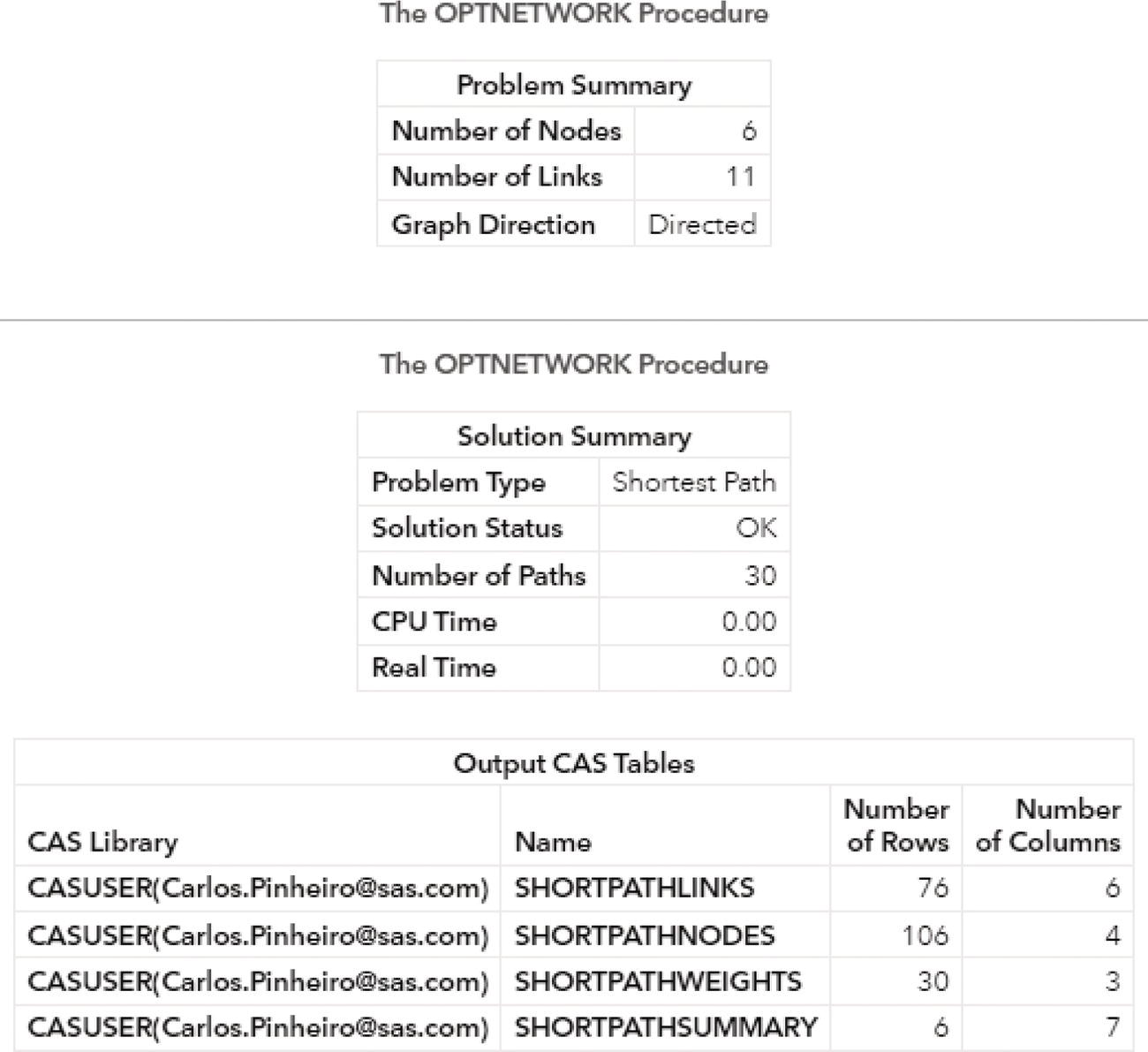
Figure 4.73 Output results by proc optnetwork running the shortest path algorithm on a directed input graph.
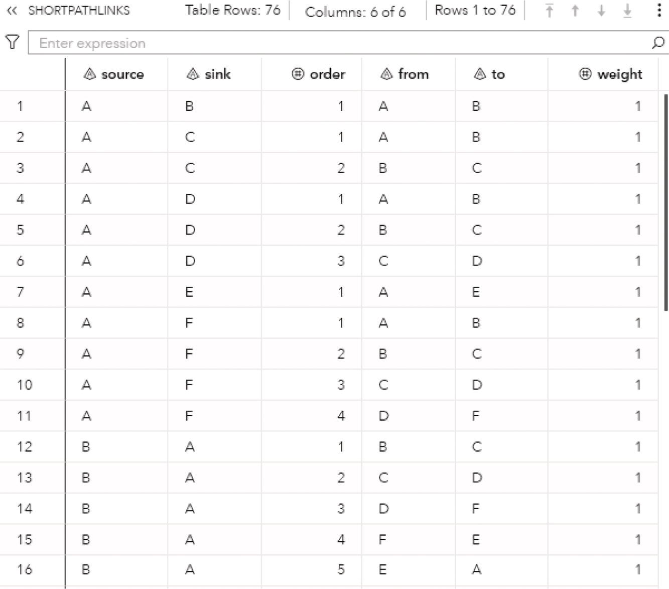
Figure 4.74 The shortest path solution for the links.
Line 1 describes a shortest path comprising one single link, from the source node A to the sink node B. Lines 2 and 3 describe a shortest path comprising two links. The source node is A, and the sink node is C. The two links comprised in this shortest path are from A to B and then from B to C. Similarly, lines 4 to 6 show a shortest path from source node A to sink node D, comprising three links, from A to B, from B to C, and finally from C to D. Notice that proc optnetwork found 30 shortest paths (in the results summary), comprising 76 links (number of rows in the output table SHORTPATHLINKS). This picture shows the first 16 rows.
The SHORTPATHNODES dataset presented in Figure 4.75 shows the variables source to identify the source node of the shortest path, the variable sink to identify the sink node of the shortest path, the variable order to identify the order of the link within the shortest path, and finally the variable node to identify the node partaking the particular shortest path.
Notice that the variable order identifies the sequence of the links where the node is. Shortest path A‐B, with a single link, has nodes A and B (lines 1 and 2). Shortest path A‐C has 2 links and 3 nodes, A, B, and C (lines 3, 4, and 5). Similarly, shortest path A‐D has 3 links and 4 nodes, A, B, C, and D (lines 6–9).
The SHORTPATHWEIGHTS dataset presented in Figure 4.76 shows all shortest paths and their sum of link weights, represented by the variables source and sink, identifying the source‐sink pair of node of the shortest path, and the variable path_weight, identifying the sum of the link weights of the shortest path.
For example, line 1 shows the shortest path A‐B with the sum of link weights equal to 1 (the weight of the single link A‐B). Lines 2 shows the shortest path A‐C and the sum of link weights equal to 2 (1 for A‐B and 1 for B‐C). Line 3 shows the shortest path A‐D and the sum of link weights equal to 3 (1 for each link within the shortest path, A‐B, B‐C, and C‐D).
Figure 4.77 shows the input graph and highlights the links A‐B, B‐C, and C‐D that partake shortest paths represented by lines 1, 2, and 3 on the previous output table.
The last output table, the SHORTPATHSUMMARY dataset, presented in Figure 4.78, shows the summary statistics for the shortest paths for each source node. It shows the variables source, identifying the source node of the shortest paths, paths, identifying the number of shortest paths from that particular source node, path_weight_min, identifying the minimum weight of shortest paths from that source node, path_weight_max, identifying the maximum weight of shortest paths from that source node, path_weight_avg, identifying the average weight of shortest paths from that source node, path_weight_std, identifying the standard deviation of weight of shortest paths from that source node, and path_weight_var, identifying the variance of weight of shortest paths from that source node.
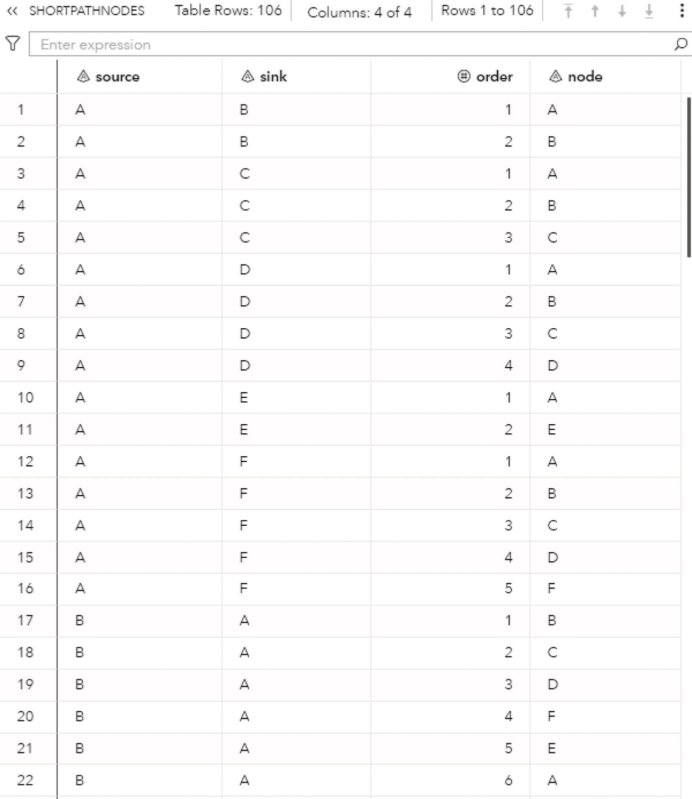
Figure 4.75 The shortest path solution for the nodes.
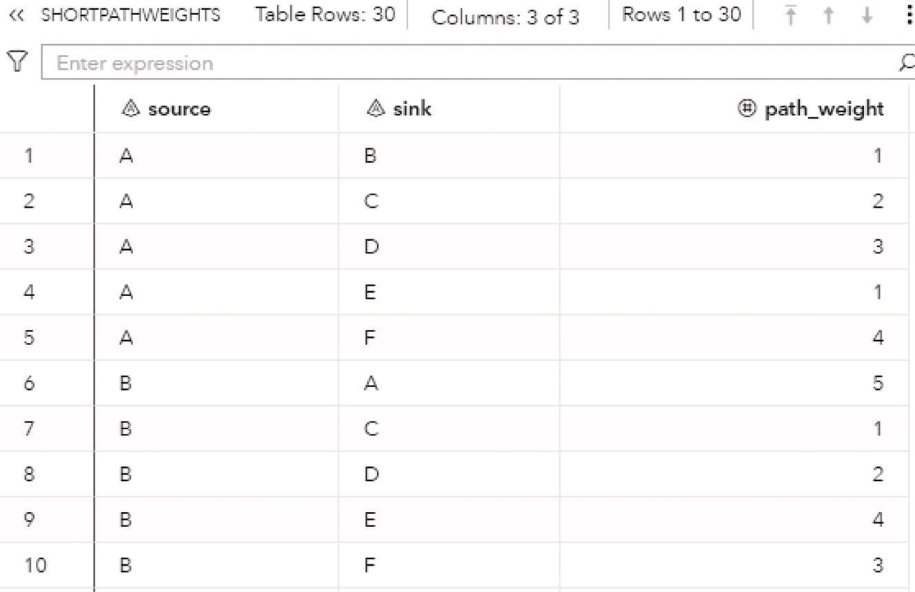
Figure 4.76 The sum of link weights of the shortest paths.
Let's see how to narrow down the search for shortest paths by defining the source and sink pairs of nodes. First, let's use the option SOURCE= to fix a particular node to tell proc optnetwork to search all shortest paths departing from that particular source node. All shortest paths returned by the shortest path algorithm will start at that node specified in the option SOURCE=. The sink nodes can be any other node in the input graph. The following code shows how to do it. For this example, the output tables to provide the summary statistics and the sum of weight links are suppressed.
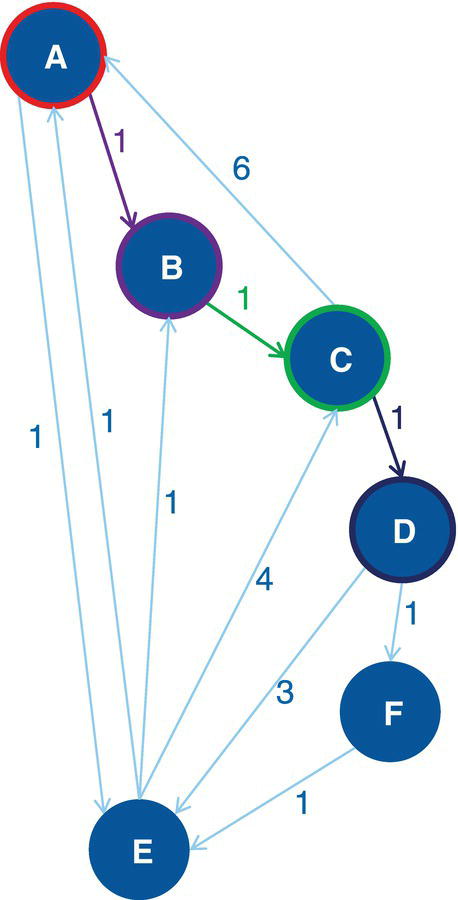
Figure 4.77 The sum of link weights of the shortest paths A‐B, A‐C, and C‐D.
proc optnetworkdirection = directedlinks = mycas.links;linksvarfrom = fromto = toweight = weight;shortestpathsource = 'A'outpathslinks = mycas.outshortpathlinksoutpathsnodes = mycas.outshortpathnodes;run;
Figure 4.79 shows the output produced by proc optnetwork. Notice that only 5 shortest paths were found when the source node is fixed as node A. Considering the entire input graph with 6 nodes being source nodes, 30 shortest paths were found.
Figure 4.80 shows the result table for the shortest path algorithm. Notice that the source node for all rows is node A. This output table shows then all the shortest paths starting at the source node A and ending at any possible sink node within the input graph.
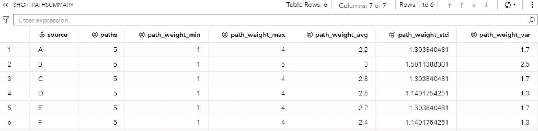
Figure 4.78 The summary statistics for the shortest path solution.
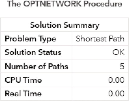
Figure 4.79 The shortest path solution with a fixed source node.
The output table OUTSHORTPATHLINKS contains all 11 links comprised by the 5 shortest paths starting at the source node A.
Let’s see now how to fix a sink node by using the option SINK=. By doing this, proc optnetwork will search for all shortest paths within the input graph that end at the sink node specified in the option SINK=. The following code shows how to define a sink node in proc optnetwork:
proc optnetworkdirection = directedlinks = mycas.links;linksvarfrom = fromto = toweight = weight;shortestpathsink = 'D'outpathslinks = mycas.outshortpathlinksoutpathsnodes = mycas.outshortpathnodes;run;
Figure 4.81 shows the output produced by proc optnetwork. Only 5 shortest paths were found when the sink node is fixed as node D.
Figure 4.82 shows the result table for the shortest path algorithm. As expected, the sink node for all rows is node D. This output table shows all shortest paths starting at any possible source node within the input graph and ending at the sink node D.
The output table OUTSHORTPATHLINKS shows all 13 links comprised by the 5 shortest paths ending at the sink node D.
Lastly, let's see how to fix both source and sink nodes when searching shortest paths and how this approach reduces dramatically the final outcomes. Proc optnetwork will search for all possible paths within the input graph where the source node is the node fixed by the option SOURCE= and the sink node is the node fixed by the option SINK=. The following code shows how to do it:
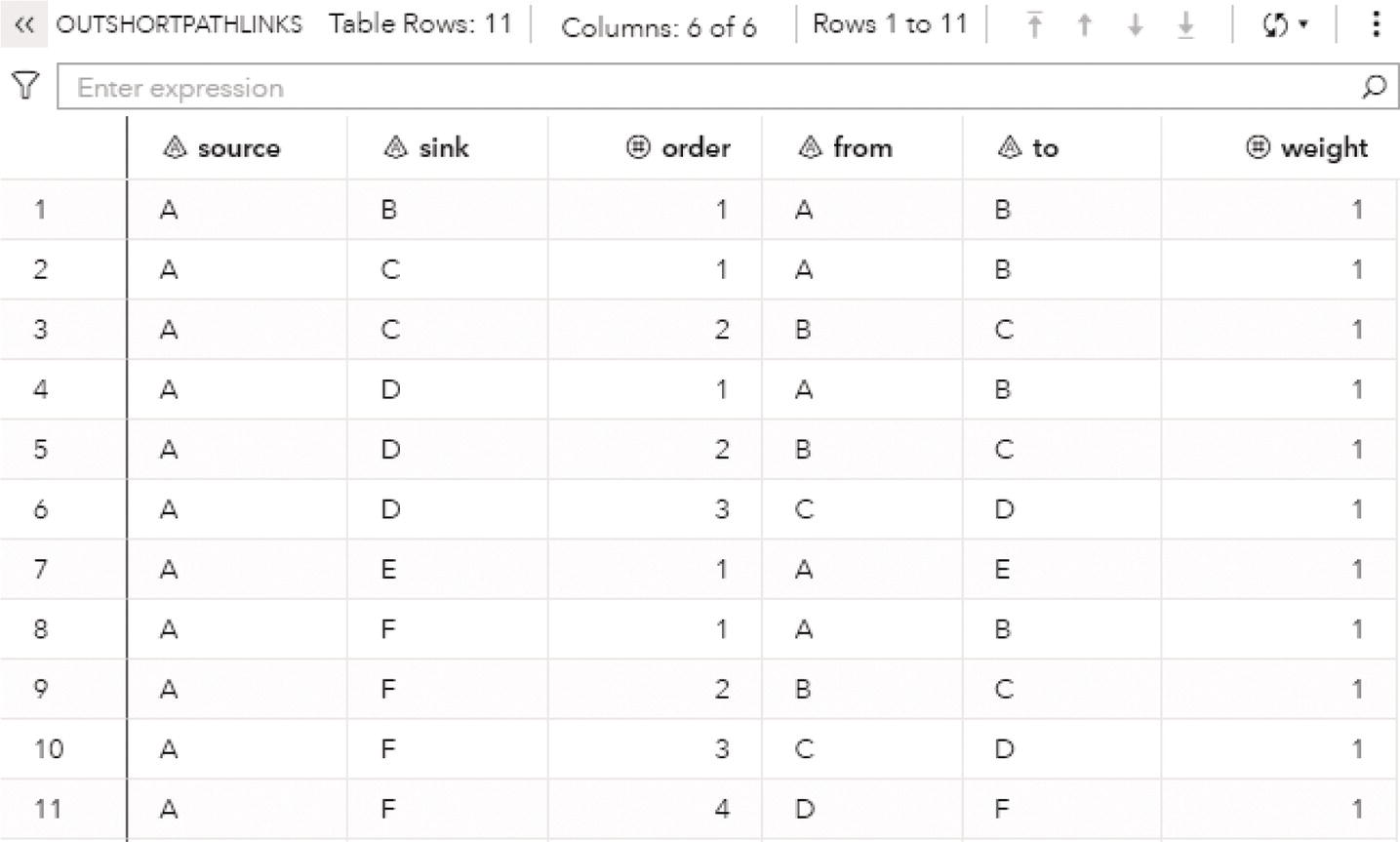
Figure 4.80 The shortest path solution for the links using a fixed source node.
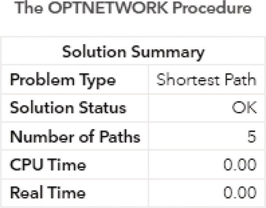
Figure 4.81 The shortest path solution with a fixed sink node.
proc optnetworkdirection = directedlinks = mycas.links;linksvarfrom = fromto = toweight = weight;shortestpathsource = 'A'sink = 'D'outpathslinks = mycas.outshortpathlinksoutpathsnodes = mycas.outshortpathnodes;run;
Figure 4.83 shows the output produced by proc optnetwork when running the shortest path algorithm for fixed source and sink nodes. As expected, by fixing both source and sink nodes, proc optnetwork returns a single shortest path, the one with the lowest sum of weight links within the input graph.
Figure 4.84 shows the result table for the shortest path algorithm. The table shows all links partaking the shortest path between the source node is A and the sink node is D.
The output table OUTSHORTPATHLINKS contains the three links comprised by the single shortest path (lowest sum of weight links) starting at source node A and ending at the sink node D.
Figure 4.85 shows the original input graph highlighting the source node A, and the sink node D, and the links partaking the shortest path between A and D.
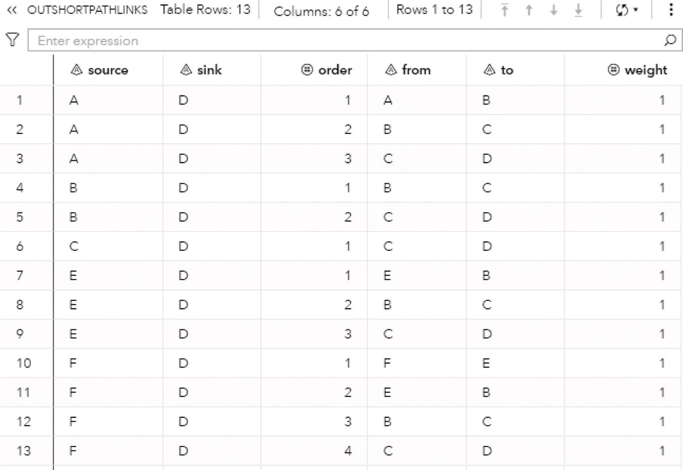
Figure 4.82 The shortest path solution for the links using a fixed sink node.
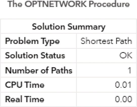
Figure 4.83 The shortest path solution for fixed source and sink nodes.
As we observed in the previous section, the path enumeration solution returned 3 possible paths between the source node A and the sink node D. The path highlighted as the shortest path between A and D is the one with the lowest sum of weight links. The path A → E → B → C → D has a total link weight equal to 4. The path A → E → C → D has a total link weight equal to 6. The path A → B → C → D has a total link weight equal to 3.
Shortest path can also be computed for undirected graphs. In that scenario, the number of shortest paths returned by proc optnetwork may be greater than the number of shortest paths returned for a directed graph just because more links will be available to connect all nodes within the input graph. This is basically due to the bidirectional aspect of the links in the input graph. A directed link A → B turns into two possible links A → B and B → A, allowing possibly more paths to be traveled.
In this example, we are also going to use different column names for the original links datasets in order to show how proc optnetwork produces the final output tables. This is also justifies the use of the LINKSVAR statement to assign the links attributes.
The input graph is the same used for the path enumeration problem. The following code creates the links dataset considering the variable a to represent the from node, the variable b to represent the to node, the variable wgt to represent the weight of the link, and the variable aux to represent the auxiliary weight for the link. As an undirected graph, the from node doesn’t necessarily represent the source node in the shortest path situation. The same for the to node. It doesn’t necessarily represent the sink node. For an undirected graph, proc optnetwork internally duplicates the links to compute all possible shortest paths considering both directions. For example, the link A → B in the links dataset will be represented by the links A → B and B → A in order to allow proc optnetwork to search for all possible shortest paths within the undirected input graph.
data mycas.links;input a $ b $ wgt aux @@;datalines;A B 1 0.5 A E 1 0.5 B C 1 0.5 C D 1 0.5 C A 6 0.17 D E 3 0.33D F 1 0.5 E A 1 0.5 E B 1 0.5 E C 4 0.25 F E 1 0.5;run;
The following code defines the direction of the input graph as well as the links attributes. The DIRECTION= option in the following code defines the input graph as an undirected graph. The LINKSVAR statement defines the variables from, to, weight and auxweight for the links when proc optnetwork searches for the shortest paths.
proc optnetworkdirection = undirectedlinks = mycas.links;linksvarfrom = ato = bweight = wgtauxweight = aux;shortestpathoutpathslinks = mycas.outshortpathlinksoutpathsnodes = mycas.outshortpathnodes;run;
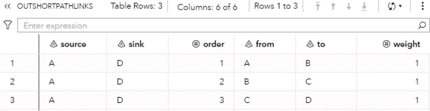
Figure 4.84 The shortest path solution for the links using fixed source and sink nodes.
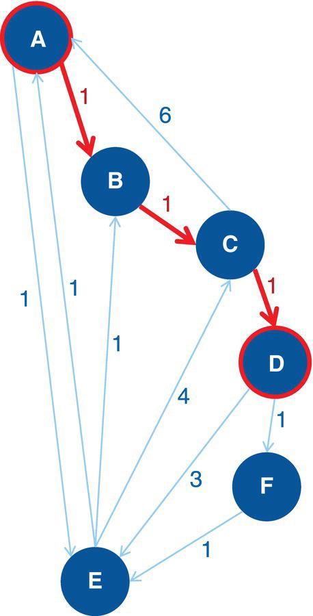
Figure 4.85 Input graph with fixed source and sink nodes.
The Figure 4.86 shows the output for the shortest path algorithm when proc optnetwork runs upon an undirected input graph. An optimal solution was achieved, and the number of shortest paths found between all possible pairs of nodes is 30, the same number found upon the directed graph.
The number of shortest paths in an undirected graph can really be greater than the number of shortest paths in a directed graph as the undirected links create more possible paths between the nodes. In this particular case, the number of shortest paths were equal based on an undirected and a directed graphs because we have here a very small network. However, something interesting is the fact the on an undirected graph, we have less links to accomplish the same number of shortest paths than on a directed graph. The reason is the same. The undirected graph creates more paths between the nodes in the input graph than the directed graphs.
Figure 4.87 shows the number of links comprised by the same 30 shortest paths when running on the directed and on the undirected graphs.
The first table refers to the directed graph and the second one refers to the undirected graph. Notice that we have 76 links comprised in the 30 shortest paths on the directed graph and just 48 links comprised in the same 30 shortest paths on the undirected graph.
Figure 4.88 shows the reason for this. As the undirected links create more straight paths between the nodes, the shortest paths between any source and sink nodes may require fewer links.
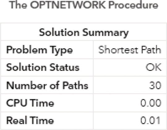
Figure 4.86 Output results by proc optnetwork running the shortest path algorithm on an undirected graph.
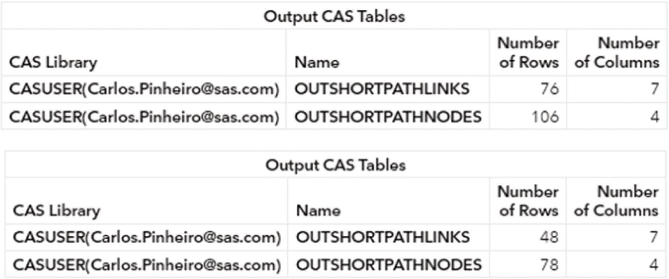
Figure 4.87 The number of links comprised in the shortest paths when proc optnetwork runs on the directed and undirected graphs.
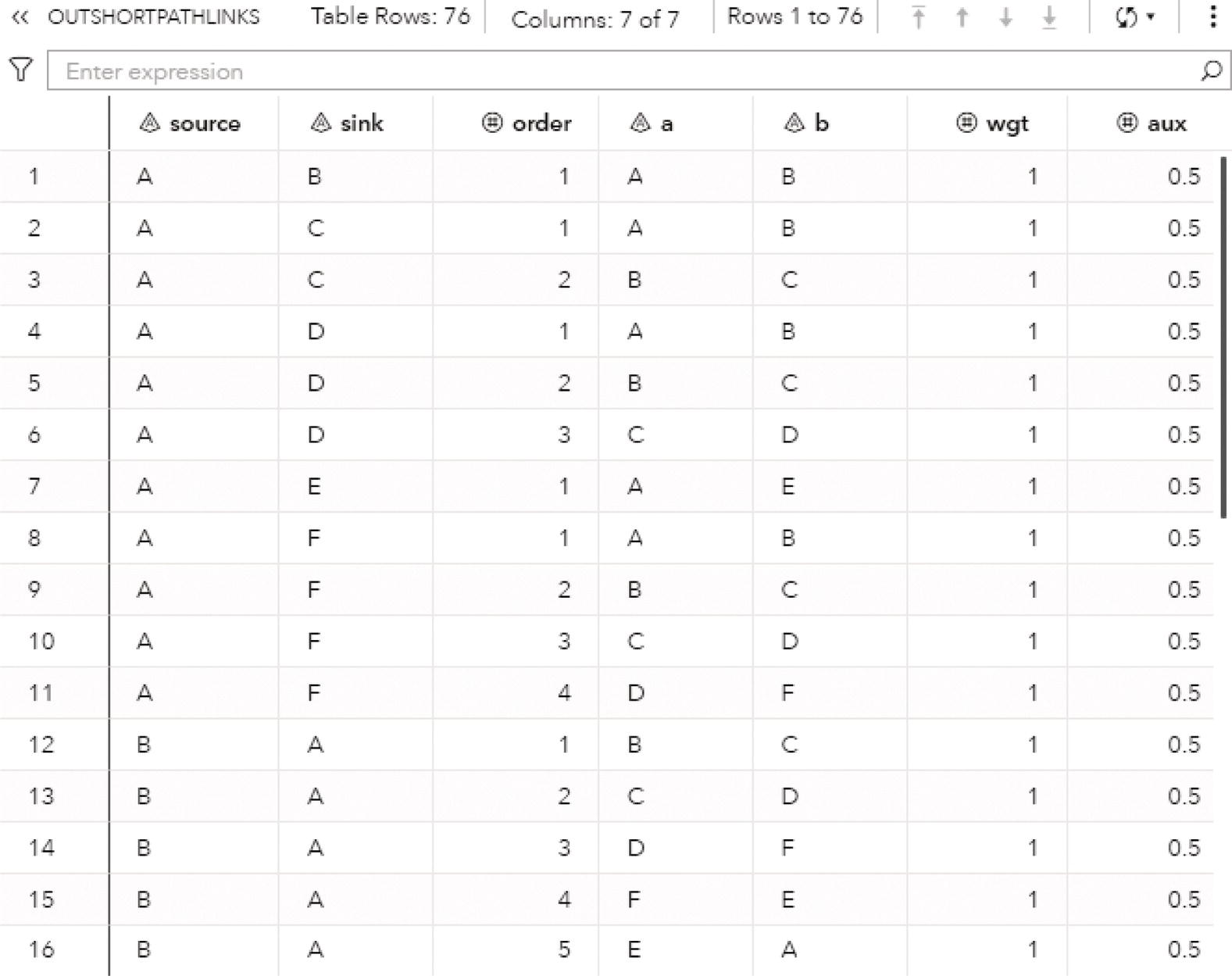
Figure 4.88 Links comprised in the shortest paths for the directed graph.
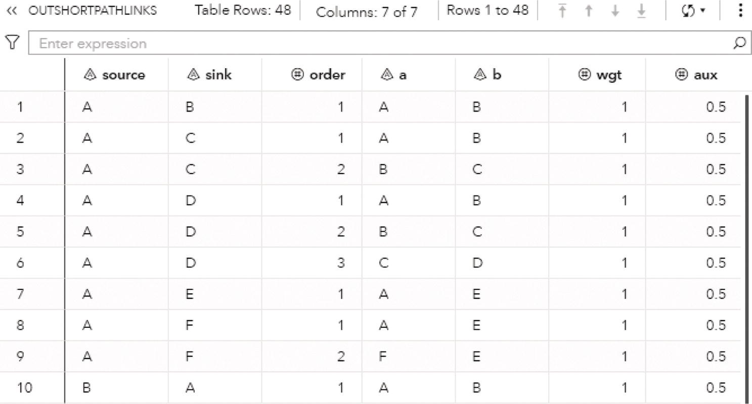
Figure 4.89 Links comprised in the shortest paths for the undirected graph.
Observe line 1 in the first table, representing the links within the shortest paths upon the directed graph. The shortest path between the source node A to the sink node B has one single link A → B. Now, observe lines 12 through 16. The shortest path between the source node B to the sink node A has 5 links, B → C, C → D, D → F, F → E and then E → A.
Now let's take a look at the shortest paths for the undirected graph. Figure 4.89 shows the links comprised in the shortest path considering the undirected graph.
In line 1 we can see the single link A → B comprised in the shortest path between the source node A to the sink node B. In line 10, we can see the single link B → A comprised in the shortest path between the source node B to the sink node A. That is the major difference between the shortest path when running on directed and undirected graphs. The original link A → B turns into 2 links A → B (the original one comprised in the shortest path between A and B) and B → A, allowing B reaches out to A directly (not passing through C, D, E, and F). The undirected graph creates more links between the nodes allowing them to reach out to each other easier, or at least, throughout shorter paths.
As mentioned before, the shortest path computation based on directed graphs tends to return less paths than when it is runs on undirected graphs. In the previous example the outcomes were similar, with 30 shortest paths for both directed and undirected paths, even though the number of total links on the directed graph was greater than the number of links on the undirected one. The reason was the size of the network. The input graph had only 6 nodes and 11 links.
The following pictures show the same scenario based on a slightly bigger network. The network here is the famous graph based on the French classic movie Les Misérables. This network has 77 nodes and 254 links. The nodes here are the actors. The links represent when the actors play scenes together. The original network is an undirected graph, as the actors play scenes together with no specific order or direction.
Figure 4.90 shows the Les Misérables's network.
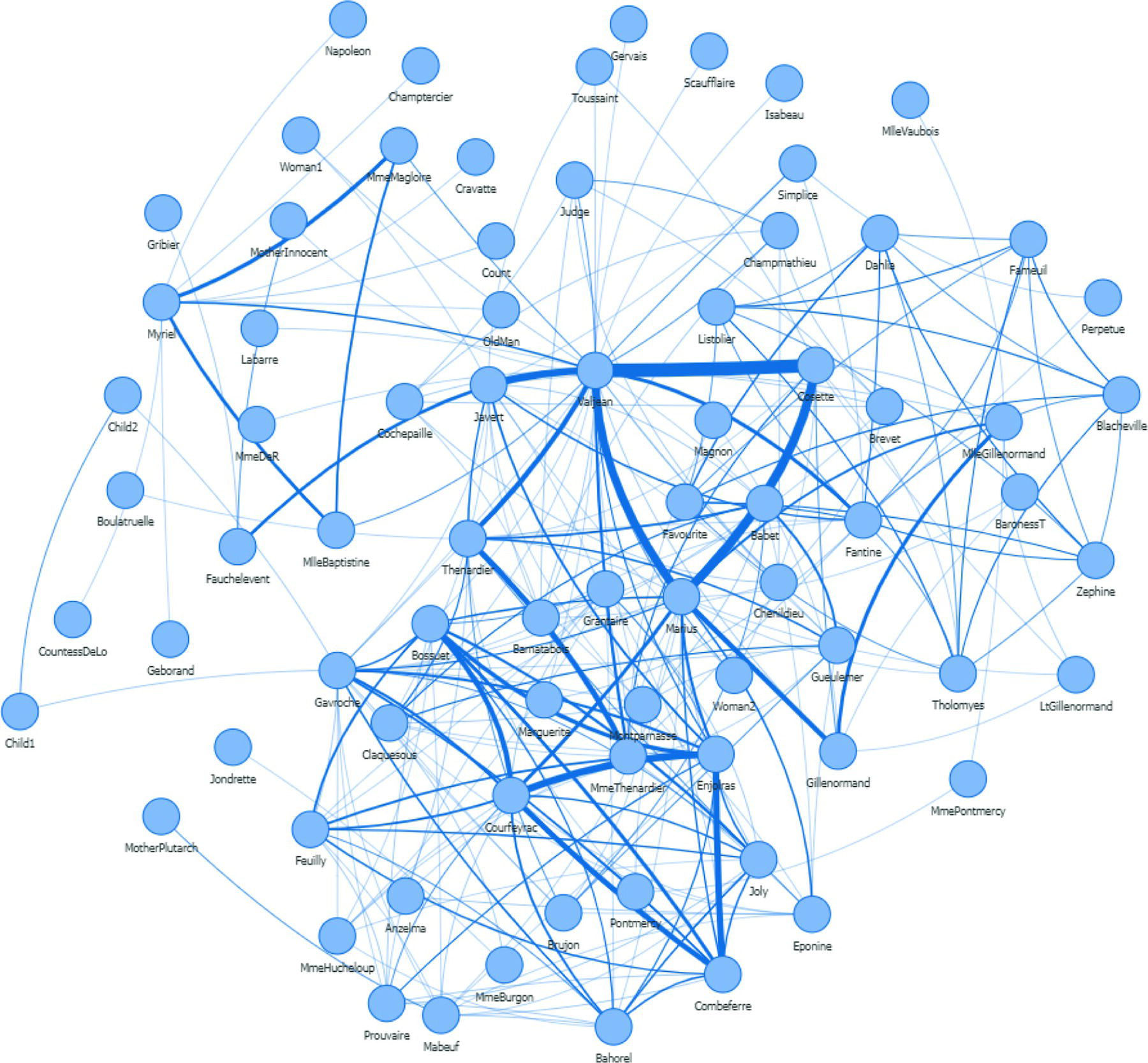
Figure 4.90 Undirected graph based on the French movie Les Misérables.
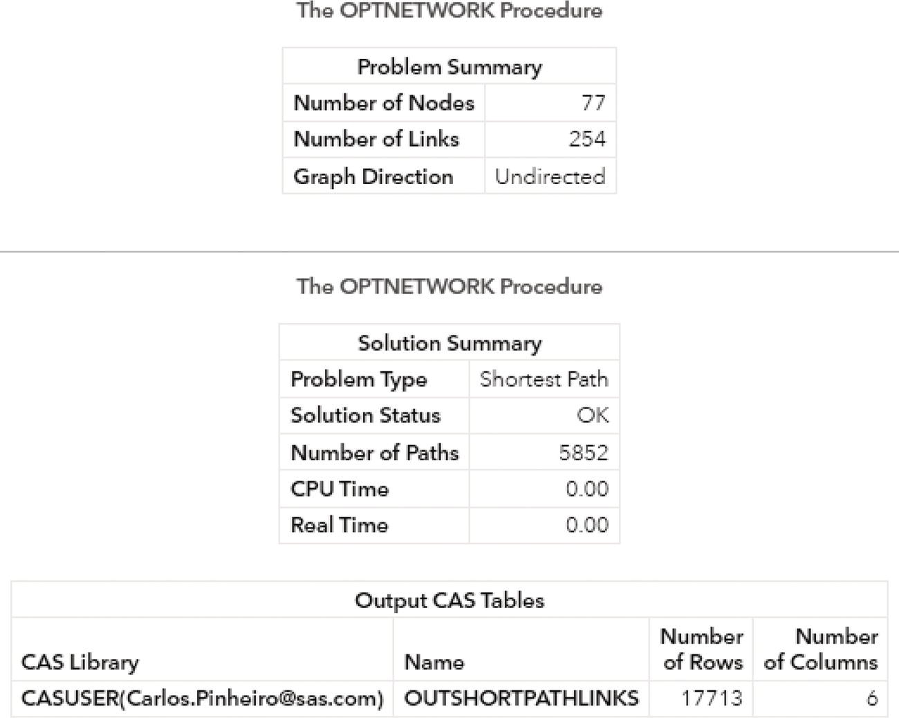
Figure 4.91 Links comprised in the shortest paths for Les Misérables's undirected graph.
Figure 4.91 shows the outcomes of the shortest path algorithm running upon the original undirected graph.
Based on the 254 links within the undirected graph, proc optnetwork found 5852 shortest paths, comprising 17 713 links between the actors.
Figure 4.92 shows the outcomes of the shortest path algorithm running upon the exact same links dataset but now set as a directed graph.
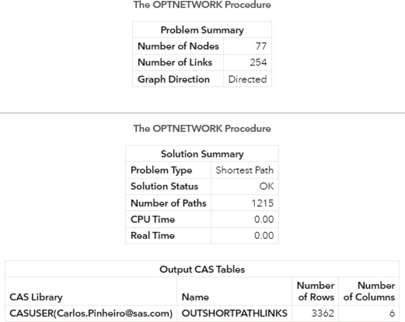
Figure 4.92 Links comprised in the shortest paths for Les Misérables's directed graph.
Now, proc optnetwork found 1215 shortest paths comprising 3362 links between the actors. As the network grows in terms of size, particularly in terms of the number of links, the difference between the number of shortest paths and the links comprised in the shortest paths tend to be very different. More shortest paths and links when running on undirected graphs.
4.11 Transitive Closure
In computer science and graph theory, transitive closure can be thought of as a concept about reachability. Can one particular node A reach node B in one or more steps considering a particular network? Transitive closure can help to efficiently answer questions about reachability between nodes within an input graph. This algorithm is commonly applied to structure query languages in database management systems in order to reduce the processing time of queries. It is also applied in problems involving reachability analysis of transition networks in distributed systems, among other applications in computer science.
The transitive closure of a graph G is a graph G T = (N, L T ) where for all nodes i, j ∈ N, there is a link (i, j) ∈ L T if and only if there is a path from node i to node j in the input graph G. In other words, the transitive closure of an input graph is a subset of links that represent binary relations between nodes. The binary relations between the nodes represent the reachability of the original input graph, or all the nodes that can reach out to each other by using one or more links in the original input graph. Eventually, a link in the transitive closure graph G T contains a link or relation that doesn't exist in the original input graph G, but the nodes witihn that relation are connected by multiple links within the original input graph. For example, an input graph has the links A → B, B → C, C → D, and D → E. The transitive closure graph has a binary relation A → E, even though the input graph does not contain that link A → E. This binary relation within the transitive closure graph is created because node A can reach out node E throughout the links A → B, B → C, C → D and D → E. Analogously, there is no link A → C, A → D, B → D, B → E, and C → E in the input graph, but the transitive closure graph contains the binary relations A → C, A → D, B → D, B → E, and C → E. The binary relation A → C goes thought the links A → B and B → C, the binary relation A → D goes thought the links A → B, B → C and C → D, binary relation B → D goes through the links B → C and C → D, the binary relation B → E goes through the links B → C, C → D, and D → E, and the binary relation C → E goes through the links C → D and D → E.
Figure 4.93 shows the input graph and the binary relations within the transitive closure graph.
The major benefit of the transitive closure algorithm is to answer questions about reachability, such as whether it is possible to reach node j from node i considering the input graph G. Given the transitive closure G T of G, it is possible thenfore to simply check for the existence of the link (i, j) in G T to answer that reachability question about how to reach node j from node i in the original input graph G. The set of binary relations describe only the nodes are reachable, for example, that node i is connected to node j no matter the number of steps or links between them. The transitive closure in that sense is another set of links.
In proc optnetwork, the TRANSITIVECLOSURE statement invokes the algorithm that solves the transitive closure problem. Proc optnetwork uses a sparse version of the Floyd‐Warshall algorithm to compute the transitive closure on a given input graph.
The output table specified in the OUT= option within the TRANSITIVECLOSURE statement contains all the links that define the transitive closure for an input graph.
Proc optnetwork computes the transitive closure for both directed and undirected graphs. As the transitive closure aims to find existing paths from one node to another within the network, the original links in the input graph (the links dataset) are “duplicated” when the direction of the graph is set to undirected. By doing this, proc optnetwork creates both directions for the links connecting a particular pair of nodes. For example, if the original links dataset defines a link A → B, when proc optnetwork computes the transitive closure based on a directed graph, that original link A → B remains unique. However, when proc optnetwork computes the transitive closure based on an undirected graph, it duplicates the original link A → B into 2 links A → B and B → A, allowing node A to reach out to node B (based on the original link), and node B to directly reach out to node A (based on the duplicated link).
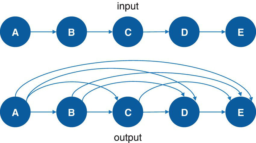
Figure 4.93 Transitive closure from a directed input graph.
4.11.1 Finding the Transitive Closure
Let's consider a very simple graph to demonstrate the transitive closure problem using proc optnetwork. Consider the graph presented in Figure 4.94. It shows a tiny network with only 5 nodes and 5 directed links. The transitive closure algorithm searches in the input graph all binary relations that represent the reachability between the nodes, which means, which nodes can reach out to other nodes within the input graph.
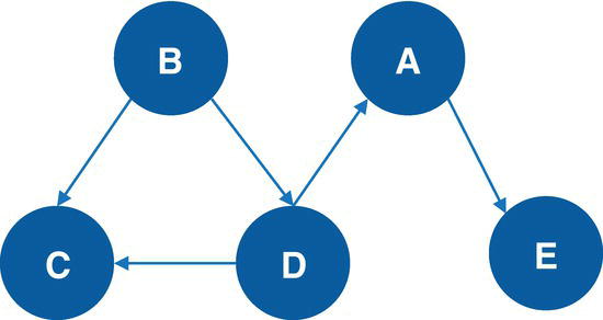
Figure 4.94 Directed input graph with unweighted links.
The following code describes how to create the links dataset that represents the input graph. In this particular case, the links represent a directed network. The links dataset has only the nodes identification, which means, the from and to variables. The link weights in the transitive closure problem are irrelevant. In other words, it doesn't matter the cost or the weight of the links, the algorithm searches for the possible paths to connect the nodes within the input graph. If there is a link or a set of links, no matter the weights, that connects node i to node j, that is the matter.
data mycas.links;input from $ to $ @@;datalines;B C B D D A D C A E;
Once the links dataset is created, we can invoke the transitive closure algorithm in proc optnetwork. The following code describes how to do it. Notice that for this particular example, we are considering the graph as directed by using the DIRECTION= option.
proc optnetworkdirection = directedlinks = mycas.links;linksvarfrom = fromto = to;transitiveclosureout = mycas.outtransclosure;run;
Figure 4.95 shows the output for the transitive closure algorithm. It says an optimal solution was found (solution status is ok) and the output table has 8 rows, representing all the binary relations between the possible connected nodes.
The next picture shows the transitive closure output table with the results. The OUTTRANSCLOSURE dataset presented in Figure 4.96 shows the original link variables from and to describing the binary relations between the nodes. Notice that this is not a set of links, but instead, it is the pairs of nodes that can be connected to each other by one or multiple links upon the original input graph.
As the network was set as a directed graph, the transitive closure algorithm follows the direction of the links in order to establish the possible paths between all pairs of nodes. Based on that, some nodes can reach out to other nodes, but cannot be reached by the same nodes. For example, node B can reach out to node C, but node C cannot reach out to node B. This happens because there is a directed link from node B to node C, but there is no directed link from node C to node B, or any sequence of links that connect node C to node B. Also notice that the number of steps or links between the nodes doesn't matter in the transitive closure solution, just the existing paths. For example, line 5 shows a binary relation between nodes B and E. There is no straight link from node B to node E, but node B can reach out to node E throughout the 3 links B → D, D → A, and A → E.
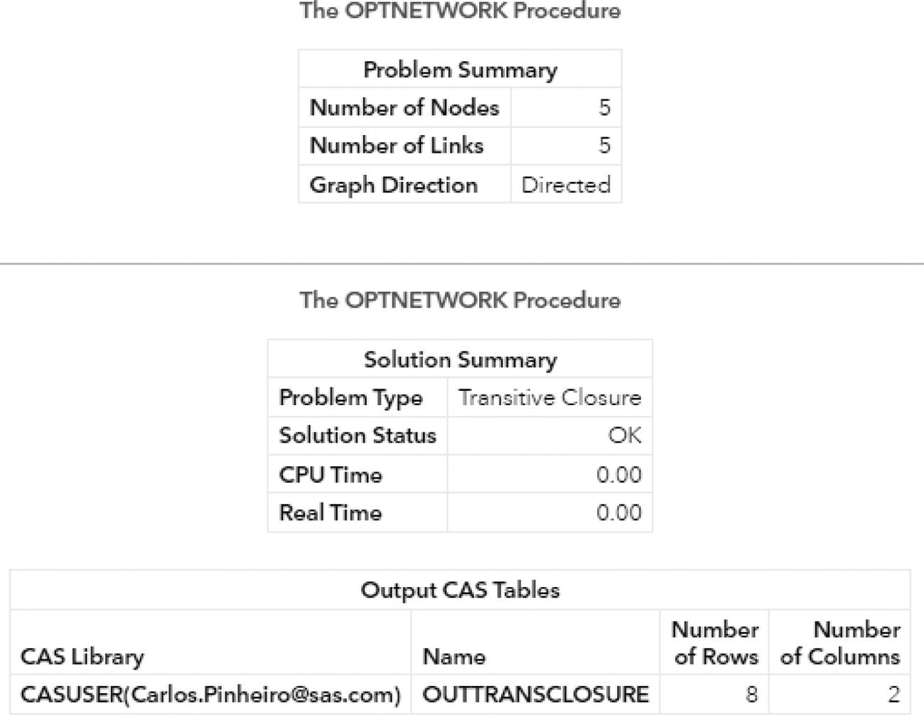
Figure 4.95 Output results by proc optnetwork running the transitive closure algorithm on a directed input graph.
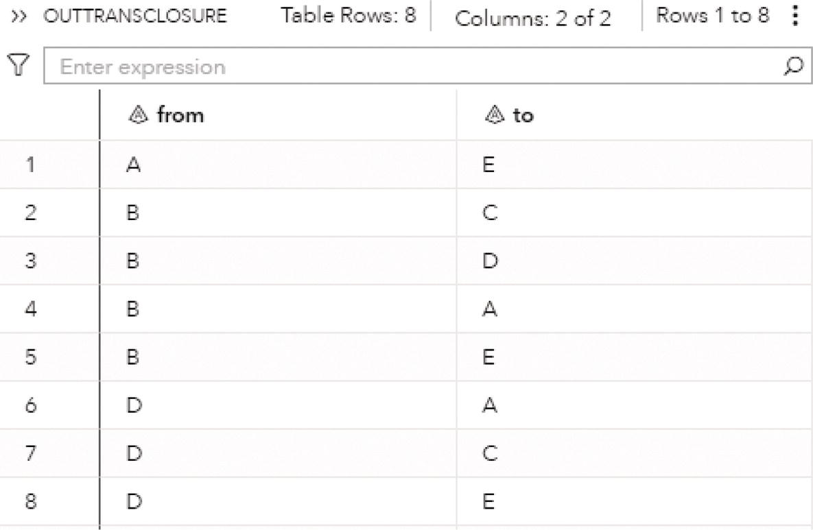
Figure 4.96 The transitive closure output.
Figure 4.97 shows the path from node B to node E throughout directed links within the input graph.
In this example, nodes C and E cannot reach out to any other node in the input graph, no matter the number of links or possible paths in the network.
This scenario certainly changes if we define the network as an undirected graph. As an undirected graph, proc optnetwork will turn all unique directed links into bidirectional links. That would create more paths within the input graph, allowing more nodes to reach out other nodes and be reached.
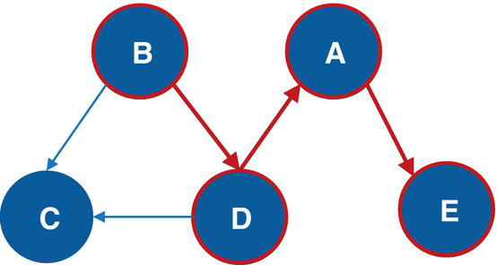
Figure 4.97 The binary relation B‐E through three directed links within the input graph.
Let's use the exact same input graph. The only modification we need to do in the code is to change the option DIRECTION= to set the graph as undirected. The following code shows that modification:
proc optnetworkdirection = undirectedlinks = mycas.links;linksvarfrom = fromto = to;transitiveclosureout = mycas.outtransclosure;run;
Figure 4.98 shows the output for the transitive closure algorithm running upon an undirected graph. Notice that we have the exact same number of nodes and links (5 for both), but the output table now has 15 rows, representing more binary relations between the nodes in the input graph.
Figure 4.99 shows the transitive closure output table with the results for the undirected graph. The OUTTRANSCLOSURE dataset shows all 15 binary relations between the nodes in the network.
As the network was now set as an undirected graph, the transitive closure algorithm follows both directions for each link defined in the links dataset. That creates more possible paths to connect the nodes within the input graph. For the directed graph, we saw that nodes C and D couldn't reach out to any other node in the network. Now, as an undirected graph, all nodes can reach out to any other node in the network.
There are two important things to notice on the results of the transitive closure for undirected graph. First, we can see that nodes can reach out to themselves. That would be auto relations, like node A can reach out to node A. That happens to all 5 nodes in the input graph. Second, as an undirected network, proc optnetwork doesn't repeat the binary relation in the output. For example, node A can reach out to all other nodes, B, C, D, and E, shown in lines 2 through 5. Node B can also reach out to all other nodes, A, B, C, D, and E. Line 6 shows the auto binary relation. Lines 7, 8, and 9 show the relations to nodes C, D, and E, respectively. Line 2 actually shows the relation to node A, as A‐B. As an undirected graph, the relation A‐B is exact the same as the relation B‐A. Therefore, there is no need to duplicate that relation as B‐A in the output table.
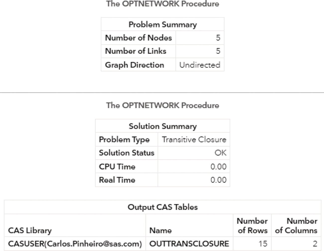
Figure 4.98 Output results by proc optnetwork running the transitive closure algorithm on a input undirected graph.
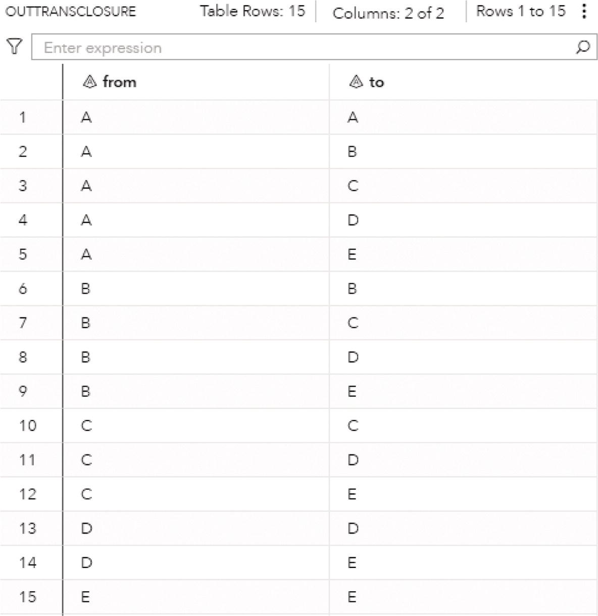
Figure 4.99 The transitive closure output for an undirected graph.
Figure 4.100 shows the undirected graph based on the bidirectional links created by proc optnetwork, and we can see that there is a path from any node to any other node in the network.
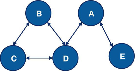
Figure 4.100 The undirected graph with bidirectional links between the nodes.
Finally, it is important to notice that the transitive closure algorithm searches for all possible combinations of paths within the input graph in order to find binary relations between the nodes, the output table can be very large if the network is large. For example, considering the network to represent the French movie Les Misérables, with only 254 links, based on an undirected graph, the transitive closure will produce an output table with 3,003 rows, representing all binary relations within the network. Figure 4.101 shows the result for the transitive closure considering the Les Misérables network.
The Les Misérables network is a very dense graph, where actors commonly play scenes together, or in terms of a graph, nodes are commonly connected. The 77 actors, or nodes, are completely connected, which means any node within that network can reach out to any other node. The combination of 77 nodes by 2 elements gives us 2926 possible binary relations. Plus, we have the 77 auto relations. That gives us the final result of 3003 rows in the output table.
4.12 Traveling Salesman Problem
The TSP aims to find the minimum‐cost tour in a given input graph. The minimum cost tour is a particular elementary cycle within the input graph. A path in a graph is a sequence of nodes linked to each other. An elementary cycle is a path where the start node and the end node are the same and no node is visited more than once in the sequence. A tour is an elementary cycle where every node within the input graph is visited once and only once. The TSP algorithm aims to find the tour with the minimum total cost. The elementary cycle that visits every node is known as the Hamiltonian Cycle. The Hamiltonian path in an undirected graph is a path that visits each node exactly once. A Hamiltonian cycle is a Hamiltonian path such that there is a link from the last node to the first node of the Hamiltonian path. There is a subtle difference between the Hamiltonian Cycle and the TSP. The Hamiltonian cycle problem aims to find a tour that visits every node exactly once within the input graph (or a subgraph within a larger network). In fact, many tours can exist in the input graph that satisfies that condition. The TSP aims to find the minimum weight Hamiltonian cycle.
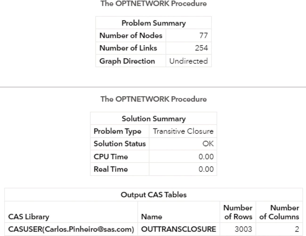
Figure 4.101 The transitive closure for the Les Misérables's network.
The TSP answer questions about optimal routes to visit a set of locations considering existing links between nodes (locations to visit) within a network. For example, given a list of locations in a city, and the distances between each pair of these locations, what is the shortest possible route that visits every selected location within the city exactly once and returns to the origin place. The origin place might be a hotel in a tourist city, and the places to visit may be a set of monuments, museums, and restaurants. The TSP searches for the optimal tour to depart from the hotel, visit all selected monuments, museums, and restaurants, and return to the hotel at the end of the tour. The optimal tour can be the total shortest distance traveled when covering all the selected places, in the shortest time, or the shortest cost. For instance, assume we have multiple transportation options to go from one place to another. We can walk, which is free, take the bus, which is cheap, take the metro, which is fast, or take the taxi, which might be more straightforward. The optimal tour can minimize the time, the distance, or the cost to travel and visit a set of locations in the city.
The TSP has applications in many areas like planning, logistics, routing, manufacturing, computer networks, astronomy, DNA sequencing, among others. TSP has an unclear origin. It was described by Willian Rowan Hamilton and Thomas Kirkman in the 1800s. The problem was mathematically formulated in the 1930s by Merrill Flood searching for a solution on school bus routing problem. The problem has been studied for decades in many fields like mathematics, computer science, chemistry, and physics, and several solutions have been theorized. The simplest solution is to try all possibilities. However, this method can be quite time consuming and exhaustive particularly in large networks. For those reasons, many solutions use heuristics, which provides probability outcomes for the possible optimal tours. The results in these cases are approximate and not always optimal. Other solutions focus more on optimization methods, which includes branch and bound, Monte Carlo, and Las Vegas algorithms to minimize the computing time while finding the optimal solutions.
Formally, the TSP finds a minimum‐cost tour in a graph G that has a node set N and a link set L. When searching for the solution, each link (i, j) ∈ L is associated with a binary variable x ij , indicating whether or not the link (i, j) is part of the tour. Additionally, each link (i, j) is also associated with another variable c ij indicating the cost of the link. The total sum of the link weight is important to define the minimum cost tour in the TSP.
The TSP can be formulated as a linear programming for an undirected graph G. The mathematical formulation is as follows:
where for each subset S of nodes δ(S) represents the set of links (i, j), with i ∈ S and j ∉ S.
The first equation represents the matching constraints, which ensure that each node has degree 2 in the subgraph. The second inequality equation represents the subtour elimination constraints, which enforce connectivity.
For a directed graph G, the same formulation and solution approach are used on an expanded graph G ′. Proc optnetwork constructs the expanded graph and returns the solution in terms of the original input graph.
In the context of network flow, we can think of the TSP as a routing problem. For example, each node is a location, and each link is a road connection to a pair of locations. The distance between the pairs of locations is the cost of the link. The goal of the TSP is to find the shortest possible route that connects all locations. Each location must be visited only once. Links can also be seen as pathways, metro, or bus lines, or any other mode of transportation. Then, the distance can be seen as cost or time. In that way, the TSP aims to find the cheapest or the shortest time route to visit all locations in the node set.
In proc optnetwork, the TSP statement invokes the algorithm that solves the TSP. This algorithm is based on a variant of the branch‐and‐cut process described in the book The Traveling Salesman Problem: A Computational Study, by David L. Applegate, Robert E. Bixby, Vašek Chvátal, and William J. Cook.
Proc optnetwork implements a linear programming‐based branch and cut algorithm. This method uses a divide and conquer approach. It attempts to solve the original problem on general mixed linear programs by solving linear programming relaxations of a sequence of smaller subproblems. The procedure also implements advanced techniques like generating cutting planes and applying primal heuristics to improve the efficiency of the overall algorithm.
There are many options for the TSP algorithm in proc optnetwork. As usual when trying to optimize (maximize or minimize) an objective function in network flow problems, something important when defining the input graph is the weight (or the cost) of the links. The option WEIGHT= in the LINKSVAR statement is used to specify the cost of the links in the input graph and used when proc optnetwork is searching for the minimum cost tour. The direction of the link in the input graph is also crucial. Proc optnetwork can compute the TSP for both directed and undirected graphs. The results of the algorithm can be very different when searching the optimal tour in directed and undirected graphs. Undirected graphs create more paths between the nodes, allowing more possible cycles within the network. Directed graphs have fewer paths within the network as the direction of the link may continue or interrupt a particular cycle. The option DIRECTION= defines the direction of the links within the network and completely changes the way proc optnetwork computes the optimal tour. For example, if we create the links dataset considering the direction of the link, in a directed graph, the from node in each link will be the origin and the to node will be the destination. That link will be unique in the network. For the same links dataset, defined as an undirected graph, the from node can be origin in one link and destination in another, and the to node can be the destination in one link and origin in another. In the directed graph the link A → B is unique and represents A as origin and B as destination. This is a single connection from A to B. In an undirected graph, the original link A → B in the link set can represent A as origin and B as destination, as well as B as origin and A as destination. The original link A → B turns into 2 links A → B and B → A describing two possible connections, from A to B and from B to A. That creates more possible paths between the nodes, which represents more possible cycles. From more possible cycles, there are more possible optimal tours within the network.
The final result for the TSP algorithm in proc optnetwork is reported and saved in the output tables defined by the options OUT= and OUTNODES=. The output table specified in the OUT= option in the TSP statement reports the optimal tour as a sequence of links. This output table contains the following variables. The variable tsp_order contains the order or the sequence of the link in the tour. The variable from contains the node label of the origin in the link. The variable to contains the node label of the destination in link. The variable weight contains the cost of the link. The cost can be the distance, the time, or the price to travel from the origin node to the destination node. The output table specified in the OUTNODES= option in the PROC OPTNETWORK statement reports the optimal tour as a sequence of nodes. This output table contains the following variables. The variable node contains the node label, and the variable tsp_order contains the order or the sequence of the node in the optimal tour.
The option ABSOBJGAP= or ABSOLUTEOBJECTIVEGAP= specifies a stopping criterion for the algorithm when searching for the optimal tour. If the absolute difference between the best integer objective and the objective of the best remaining branch‐and‐bound node becomes less than the value specified in the option, the solver stops searching for more solutions. The value of number specified in the option can be any nonnegative number. The default t value is 1E–6.
The option RELOBJGAP= or RELATIVEOBJECTIVEGAP= specifies a stopping criterion for the algorithm when searching for the optimal tour. This stopping criterion is based on the best integer objective and the objective of the best remaining node. The relative objective gap is the difference between the best integer objective and the objective of the best remaining node divided by the objective of the best remaining node. When the relative objective gap becomes less than the number specified in the option, the solver stops searching for an optimal solution. The value of number can be any nonnegative number. By default, the option RELOBJGAP= is set to 0.0001.
The option TARGET= specifies a stopping criterion for minimization problems. If the best integer objective is less than or equal to the number specified in the option, the solver stops searching for an optimal solution for the TSP tour. The value of the number specified in the option can be any number. The default is the largest negative number in magnitude that can be represented by a double.
The option CUTOFF= specifies the cutoff value for any branch‐and‐bound nodes in a minimization problem. The main idea of the cutoff is the following. If the optimal linear programming relaxation objective is not better than the cutoff value specified, then any mixed integer programming solution of a descendant can be no better than the cutoff. Then the node in the branch‐and‐bond method can be fathomed and does not need to be further considered in the search. If the objective value is greater than or equal to the number specified in the option, the algorithm stops the branch‐and‐bound search. The default is the largest number that can be represented by a double.
The option CUTSTRATEGY= specifies the level of mixed integer linear programming cutting planes to be generated. The cutting plane method iteratively refines the feasible set of solution values or the objective function by means of linear inequalities, also called as cuts. This method is commonly used to find integer or mixed integer solutions in linear programming. The cutting plane method works by solving a non‐integer linear program by using a linear relaxation of the given integer program. Specific cutting planes are always generated by proc optnetwork when searching for optimal tours in input graphs. There are four options for the cutting strategy in proc optnetwork. The option AUTOMATIC generates cutting planes on the basis of a strategy that is determined by the mixed integer linear programming solver. The option NONE disables the generation of mixed integer linear programming cutting planes (some TSP‐specific cutting planes are still active for validity). The option MODERATE uses a moderate cutting strategy. Finally, the option AGGRESSIVE uses an aggressive cutting strategy. By default, proc optnetwork disables the generation of mixed integer linear programming cutting planes by using the option CUTSTRATEGY= NONE.
The option HEURISTICS= determines how frequently to apply primal heuristics during the branch‐and‐bound tree search. The application of primal heuristics to improve algorithm efficiency affects the maximum number of iterations that are allowed in iterative heuristics. Some computationally expensive heuristics might be disabled by the solver at less aggressive levels. There are five levels of how frequent proc optnetwork applies primal heuristics during the tree search. The option AUTOMATIC applies the default level of heuristics. The option NONE disables all primal heuristics. The option BASIC applies basic primal heuristics at low frequency. The option MODERATE applies most primal heuristics at moderate frequency. Finally, the option AGGRESSIVE applies all primal heuristics at high frequency. By default, the level of primal heuristics application in the tree search is AUTOMATIC.
The option LOGFREQ= or LOGFREQUENCY= specifies the time interval in seconds for printing information in the node log during the branch‐and‐bound algorithm. The node indicates the sequence number of the current node in the search tree. The number specified in the option can be any integer greater than or equal to zero. If the option is specified as 0, the node log is disabled. If the option is specified with any number greater than 0, the root node processing information is printed and, if possible, an entry is made at every number of seconds specified in the option. An entry is also made each time a better integer solution is found. By default, the option LOGFREQ= is specified at 5, which means, printing information in the node log at every five seconds.
The option MAXNODES= specifies the maximum number of branch‐and‐bound nodes to be processed. The default is any nonnegative integer that can be represented by a 32‐bit integer. When running the mixed integer liner programming in concurrent mode, the solver stops as soon as the number specified in the option is reached on any machine. When running the mixed integer linear programming algorithm in distributed mode, the solver periodically checks the total number of nodes that are processed by all grids and stops when the number specified in the option is reached.

Figure 4.102 Undirected input graph with weighted links.
The option MAXSOLS= specifies a stopping criterion. When the number of solutions specified in the option is found, the procedure stops searching for new optimal solutions. The default is the largest number that can be represented by a 32‐bit integer.
The option MAXTIME= specifies the maximum amount of time to spend solving the TSP. The type of time can be either CPU time or real‐time. The type of time is determined by the value of the TIMETYPE= option in the proc optnetwork statement. The default is the largest number that can be represented by a double. The maximum time limits the optimization process, including the problem generation and the solution time. If the MAXTIME= option is not used, the solver does not stop based on the amount of time elapsed during the optimization process.
The option MILP= specifies the type of algorithm proc optnetwork uses to find the optimal TSP tour. Proc optnetwork might or might not use a mixed integer linear programming solver. The mixed integer linear programming solver attempts to find the overall best tour by using the branch‐and‐cut algorithm. This algorithm can be expensive for large‐scale problems. The value TRUE in the option MILP= specifies the mixed integer linear programming solver as the algorithm used by proc optnetwork. The option FALSE determines proc optnetwork to use its initial heuristics to find a feasible, but not necessarily optimal tour, as quickly as possible. By default, proc optnetwork uses the mixed integer linear programming approach based on the branch‐and‐cut algorithm (option MILP = TRUE).
4.12.1 Finding the Optimal Tour
Let's consider a simple graph to demonstrate the TSP using proc optnetwork. Consider the graph presented in Figure 4.102. It shows a network with just 9 nodes and only 17 links. First, we assume this network as an undirected graph in order to compute the optimal tour to visit all nodes exactly once. Later, we assume the same network as a directed graph to see how the outcomes for the TSP can be different depending on the direction of the input graph.
The following code describes how to create the input dataset for the TSP. The links dataset has the nodes identification, the from and to variables indicating origin and destination of the possible paths within the tour, and the weight of the link, which is used by proc optnetwork to search the minimum cost tour to visit all nodes in the network. This dataset can be used to represent both directed and undirected graph as we will see in the following examples.
data mycas.links;input from $ to $ weight @@;datalines;G F 11 F D 6 F E 8 D A 12 D B 9 D H 2 D E 5 H A 3 A B 17B C 8 B E 7 C E 15 I C 4 I H 45 E I 3 E G 9 I G 32;run;
With the links dataset defined, we can now use the TSP algorithm in proc optnetwork. The following code describes how to invoke the algorithm. The links definition using the LINKSVAR statement specifies the variables from and to as the origin and destination of possible paths within the network, and the variable weight as the cost to travel through that possible path. The input graph in this example is defined as an undirected network. In that case, proc network creates two possible directions for each. For example, first link (G, F) internally turns into two distinct links (G, F) and (F, G).
proc optnetworkdirection = undirectedlinks = mycas.linksoutnodes = mycas.nodesetout;linksvarfrom = fromto = toweight = weight;tspout = mycas.tsptour;run;
Figure 4.103 shows the output for the TSP algorithm. It shows the size of the input graph, 9 nodes and 17 links. Later it says that an optimal solution was found (solution status is optimal), one single solution was found (number of solutions 1), and the objective value is 63. This value represents the cost of the optimal tour, the sum of link weights to visit all nodes exactly once.
The following pictures show the detailed results of the TSP generated by proc optnetwork. The NODESETOUT dataset presented in Figure 4.104 shows the variable node that identifies the node label and the variable tsp_order that identifies the order of the optimal tour. Note that the TSP represents a tour that visits all nodes within the network exactly once. The tour is a cycle where all nodes must be visited once and only once. As a cycle, there is no starting or ending point. The optimal tour can start at any node within the input graph.
For example, the sequence of the optimal tour starts with node A, then goes to node B, C, I, E, G, F, D, and then H. However, the sequence can actually start at node E, then to G and so forth. There is a sequence that needs to be followed, but no starting point.
The TSPTOUR dataset presented in Figure 4.105 shows the variables tsp_order that specifies the sequence of the links to be traveled in order to cover all nodes within the input graph, and the original link variables, from and to to identify origin and destination for each step of the path, and the variable weight to identify the cost of each of those steps.
Figure 4.106 shows the solution for the TSP algorithm considering the undirected input graph.
Following from the top of the input graph, the optimal tour departs from node G, goes to F, then D, H, A, B, C, I, E, and then returns to G to complete the cycle.
Let's now consider the same network but as a directed graph. The links dataset is created exactly as shown before. The only difference is the direction of the network defined in the DIRECTION= option in the proc optnetwork statement. Based on the links definition, the input directed graph looks like the following picture. For example, the definition of the first link in the data step creates the link (G, F, 11). As a directed graph, the link G → F is unique. Proc optnetwork will not create a link F → G as it did for the undirected graph.
Figure 4.107 shows the input graph considering directed weighted links.
Based on that link set definition, we can now run the proc optnetwork to search for the optimal tour invoking the TSP algorithm.
proc optnetworkdirection = directedlinks = mycas.linksoutnodes = mycas.nodesetout;linksvarfrom = fromto = toweight = weight;tspout = mycas.tsptour;run;
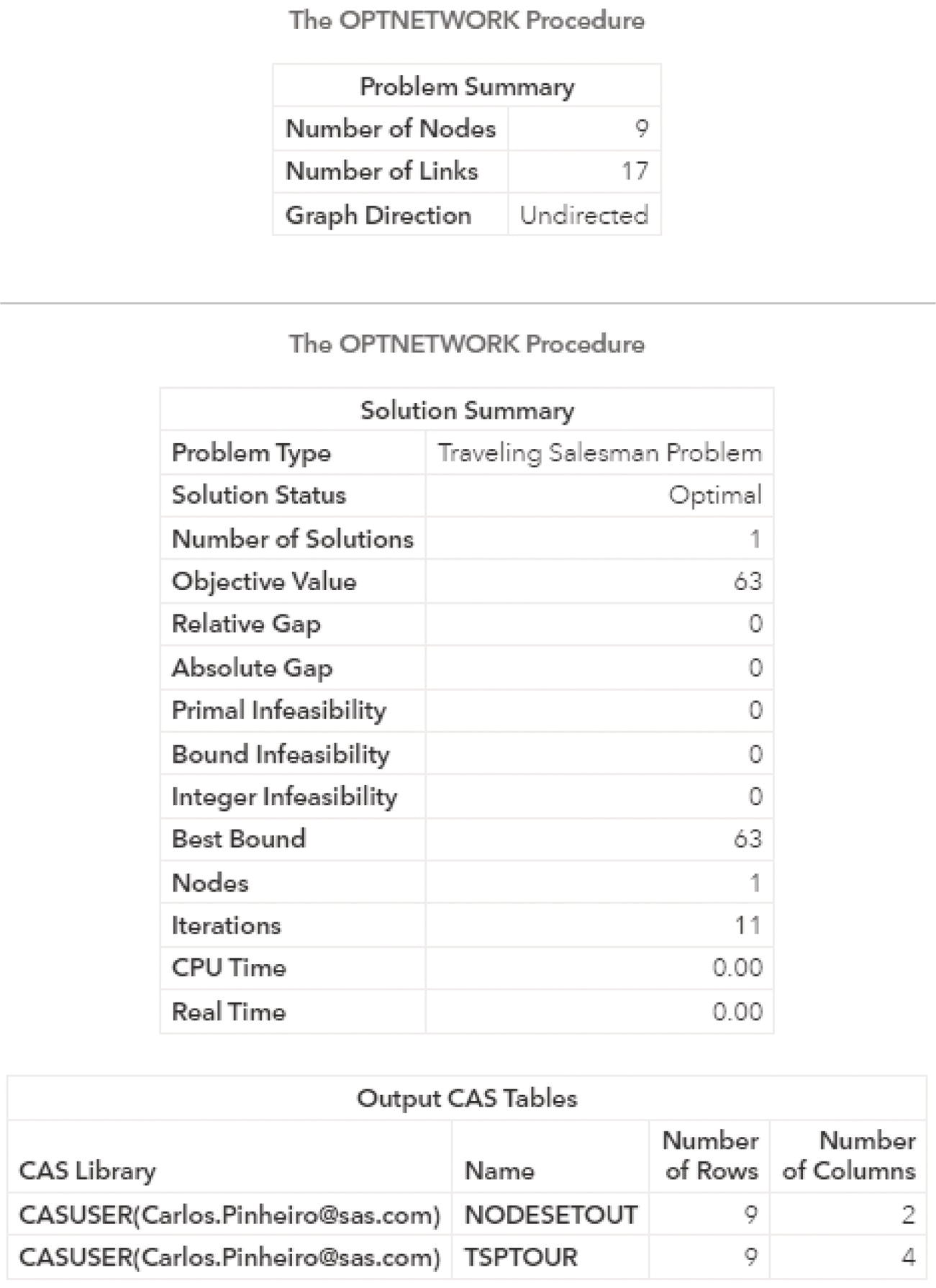
Figure 4.103 Output results by proc optnetwork running the traveling salesman algorithm based on an undirected input graph.
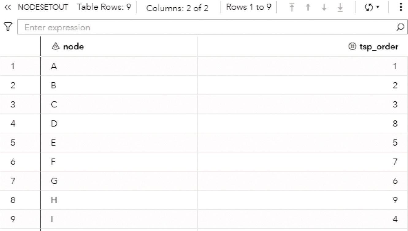
Figure 4.104 The sequence of nodes in the traveling salesman problem output based on an undirected graph.
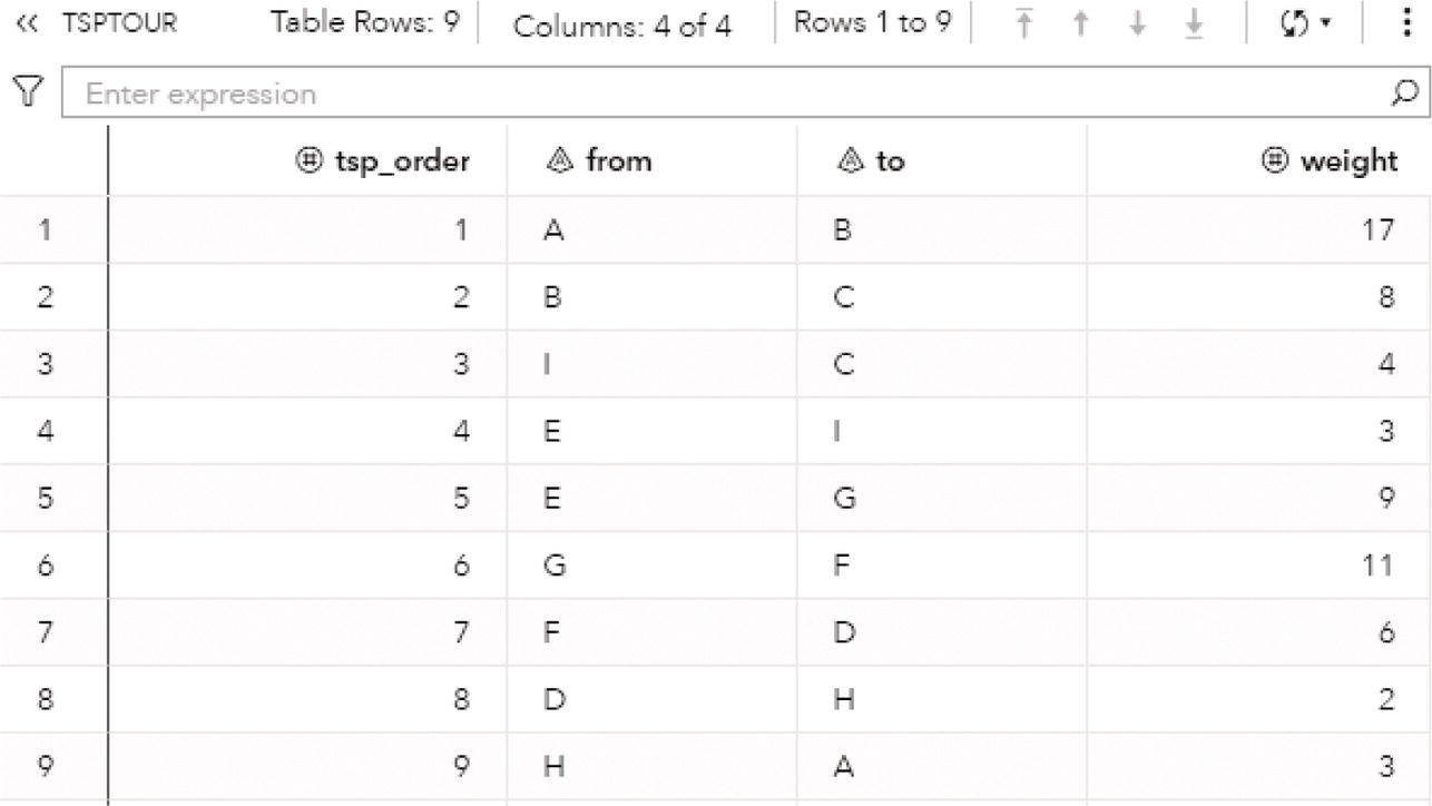
Figure 4.105 The sequence of links in the traveling salesman problem output based on an undirected graph.
Figure 4.108 shows the summary result produced by proc optnetwork. The output for the TSP based on the directed graph is very similar, except by the objective value. Recall that the objective value based on the undirected graph was 63. Now, based on the directed graph, the objective value is 97. A substantial difference. The reason for this high‐cost tour is the absence of some of the paths that were created by the undirected graph. Now the tour has unique link directions to follow from node to node, and the final tour might end up with a higher total link weight, just because some of the paths used before are not available now.
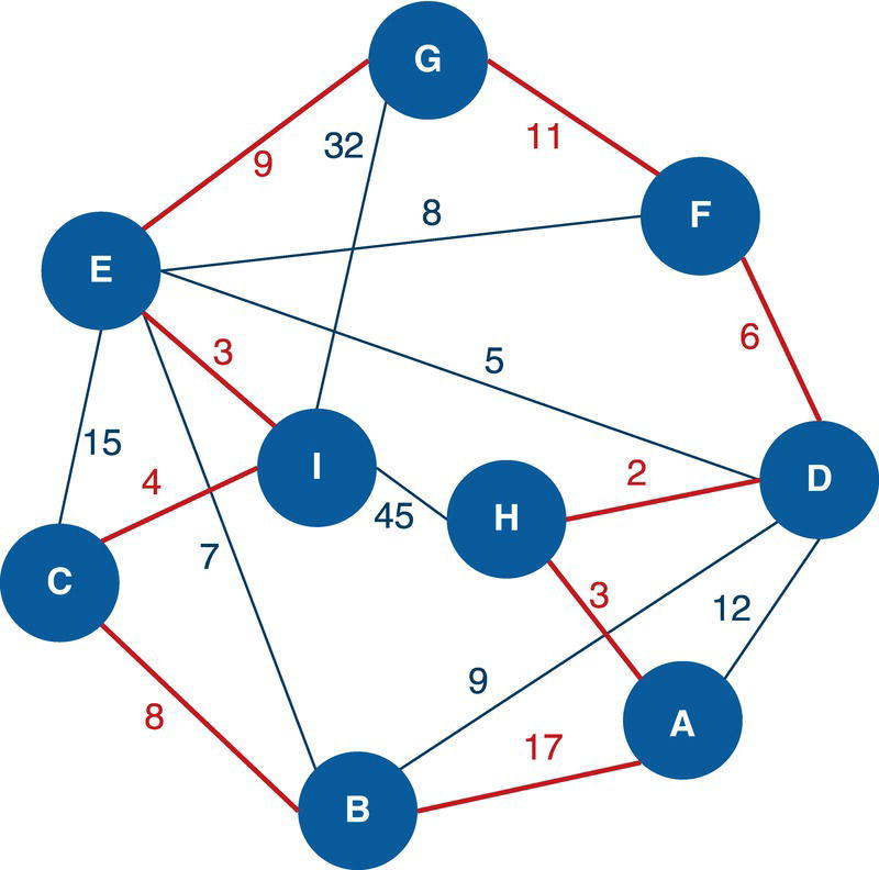
Figure 4.106 The optimal tour generated by proc optnetwork based on an undirected graph.
Figure 4.109 shows the NODESETOUT dataset that identifies the node label and the order of the optimal tour. The sequence of nodes in the TSP solution now is slightly different than before, created for the undirected graph.
The optimal tour for the undirected graph was A − B − C − I − E − G − F − D − H. Now, for the directed input graph, the sequence is A → B → C → E → I → G → F → D → H.
Figure 4.110 shows the TSPTOUR dataset that identifies the sequence of the links used to visit all nodes during the optimal tour.
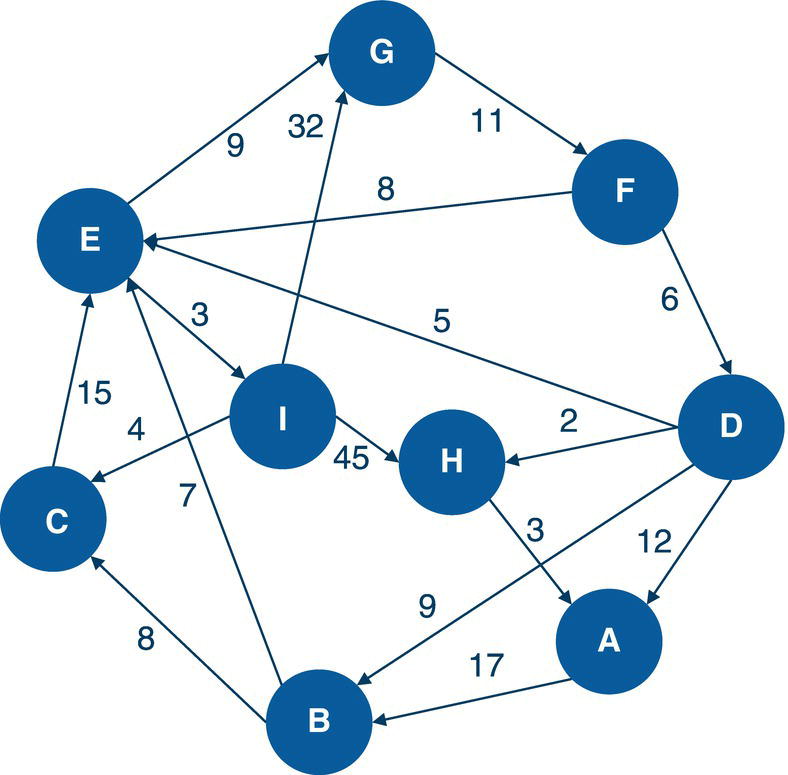
Figure 4.107 Directed input graph with weighted links.
For the undirected graph, the tour used the links C − I, I − E, E − G. That path from node C to node G cost 16 (4 + 3 + 9). However, for the directed graph, there is no link C → I neither I → E. The option for the tour is to go from C to E, costing 15, then from E to I, costing 3, and finally from I to G costing 32. The total cost for the same path is now 50, 34 more than the path for the undirected graph (16). That is exactly the difference in the objective values between the directed (97) and undirected (63) graphs.
Figure 4.111 shows the solution for the TSP algorithm considering the directed input graph.
Following from the top of the input graph, the optimal tour departs from node G, goes to F, then D, H, A, B, and C. That path so far is exactly the same as the one we saw in the undirected graph. Here resides the difference between the solutions for the directed and undirected graphs. From node C, the tour now goes to node E (not I), then node I (not E), and then goes back to node G. As we saw, because of this small difference, the optimal tour based on the directed graph costs 34 more than the tour for the undirected graph.
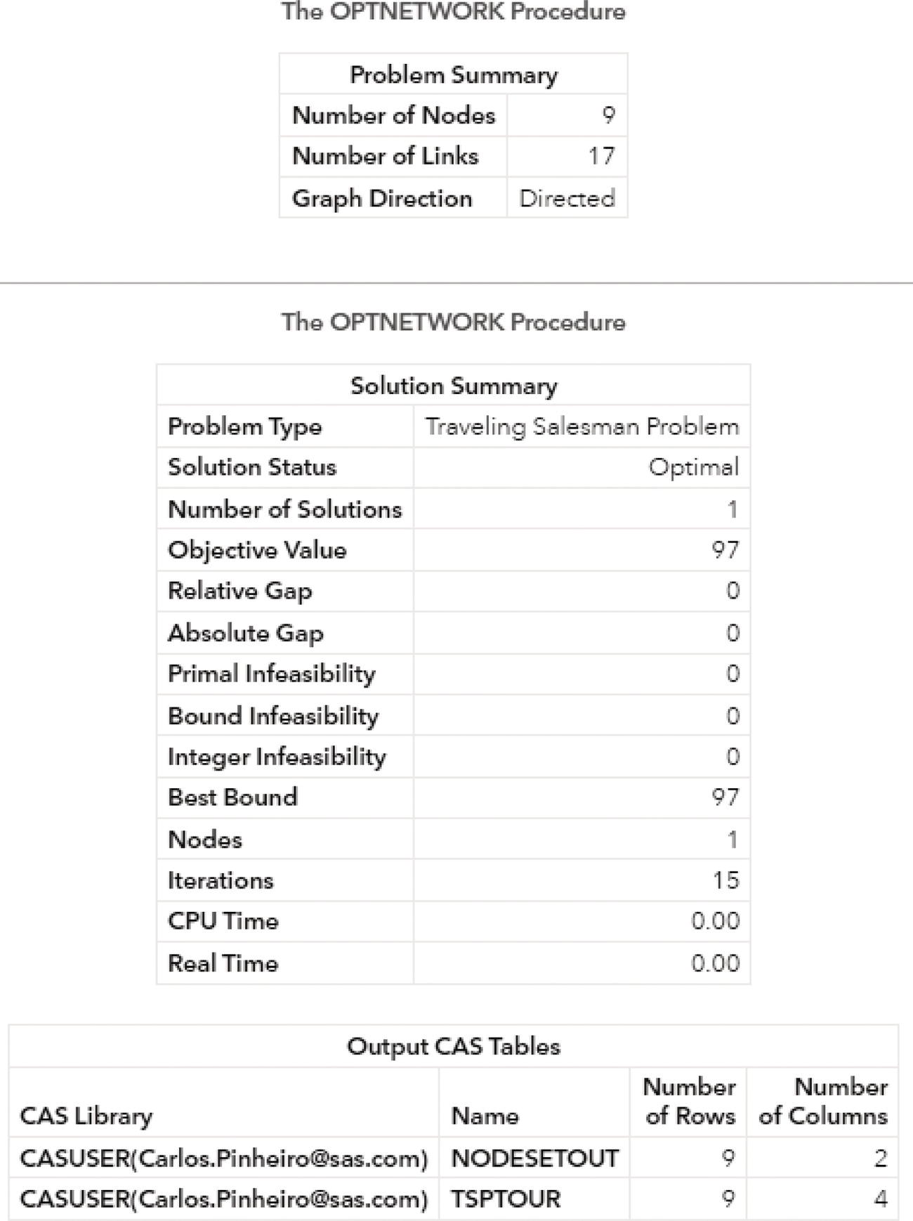
Figure 4.108 Output results by proc optnetwork running the traveling salesman problem algorithm based on a directed input graph.
Let's change the original links dataset just a tiny bit and rerun proc optnetwork for both undirected and directed graphs. We keep the exact same set of links, but we invert the order of the nodes in the link (H, A, 3). In the following data step, we create the same links set, but with the link (A, H, 3).
data mycas.links;input from $ to $ weight @@;datalines;G F 11 F D 6 F E 8 D A 12 D B 9 D H 2 D E 5A H 3A B 17 B C 8 B E 7 C E 15 I C 4 I H 45 E I 3 E G 9 I G 32;run;
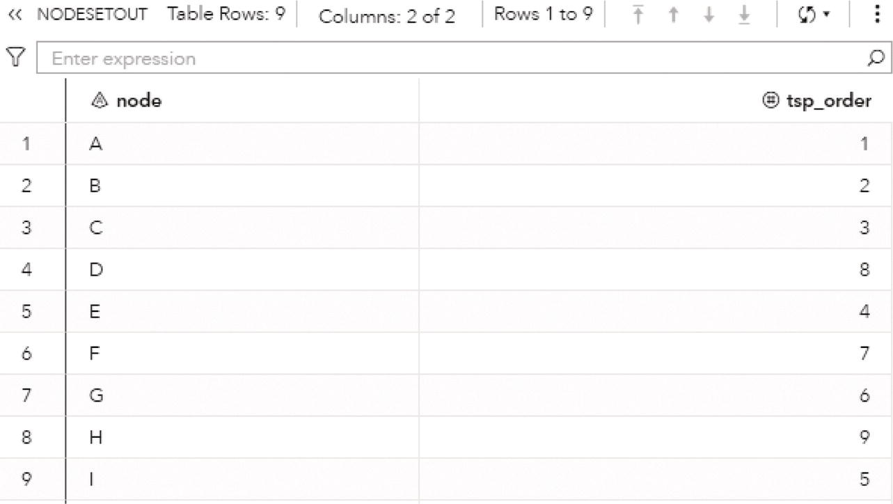
Figure 4.109 The sequence of nodes in the traveling salesman problem output based on a directed graph.
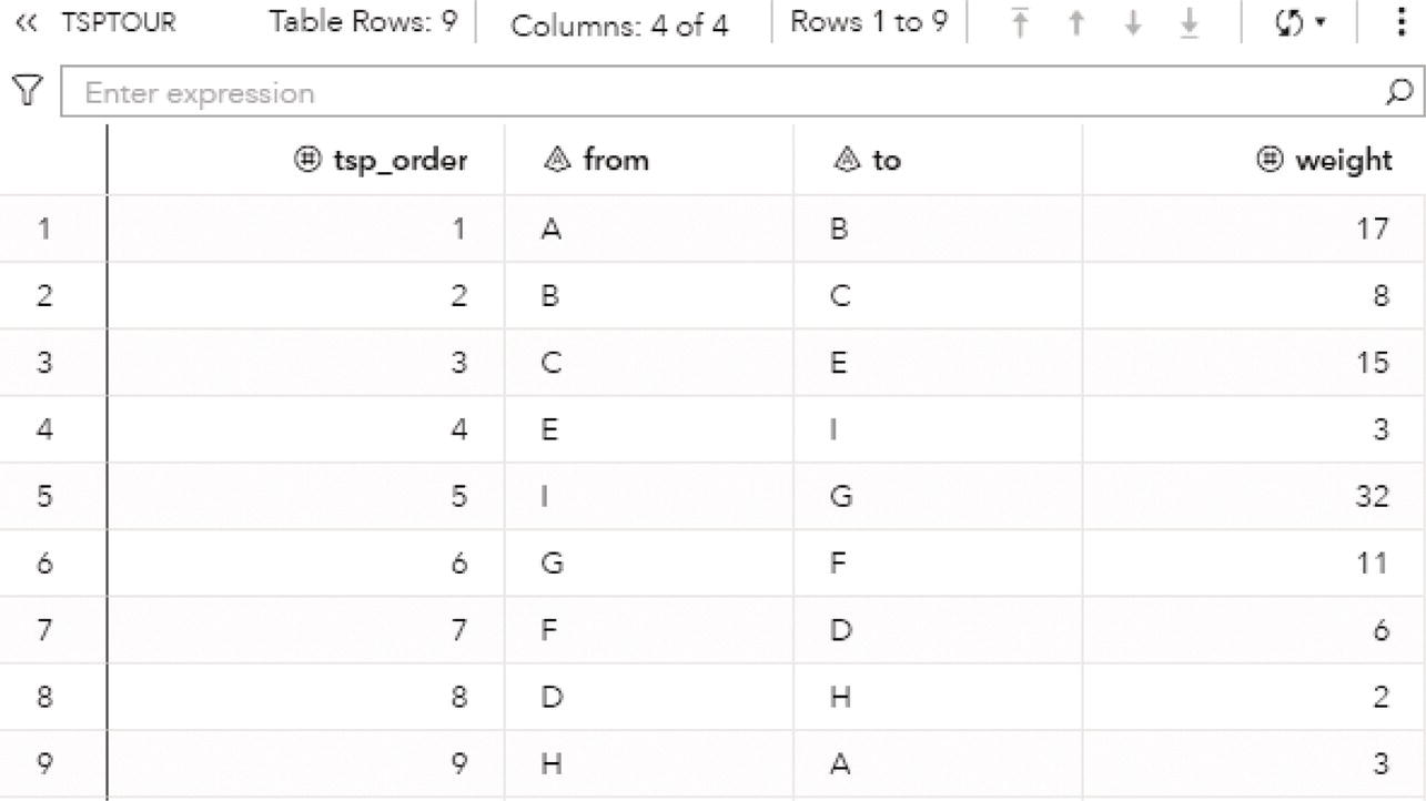
Figure 4.110 The sequence of links in the traveling salesman problem output based on a directed graph.
If we run proc optnetwork based on an undirected graph, the results will be exactly the same as we found before. The objective value is 63 and the same sequence A − B − C − I − E − G − F − D − H will be recommended. The reason is simple. On an undirected graph, it does not matter if we define (H, A) or (A, H) in the links dataset. Both directions will exist in the input graph when proc optnetwork searches for the optimal tour.
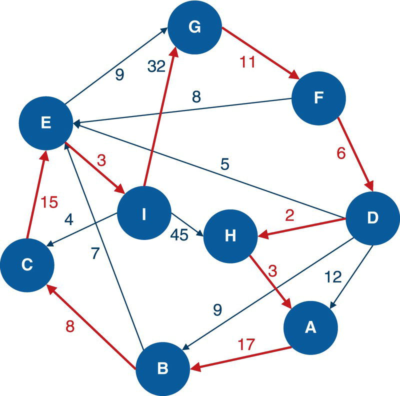
Figure 4.111 The optimal tour generated by proc optnetwork based on a directed graph.
proc optnetworkdirection = undirectedlinks = mycas.linksoutnodes = mycas.nodesetout;linksvarfrom = fromto = toweight = weight;tspout = mycas.tsptour;run;
Figure 4.112 shows the outcomes from proc optnetwork.
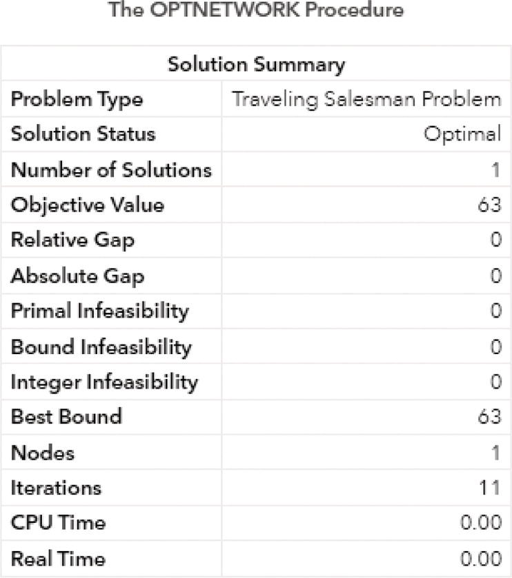
Figure 4.112 Output results by proc optnetwork running the traveling salesman algorithm based on an undirected input graph with the link ( A , H , 3).
However, if we execute the TSP in proc optnetwork based on a directed graph, because of this tiny change, the solution is infeasible.
proc optnetworkdirection = directedlinks = mycas.linksoutnodes = mycas.nodesetout;linksvarfrom = fromto = toweight = weight;tspout = mycas.tsptour;run;
Figure 4.113 shows the new input graph based on directed links.
Notice that if we follow the original sequence based on the directed graph, we start at node G, then we go to node F, and then node D. From node D, there are 3 options, nodes H, E, and A. If we go to node H, we get stuck. There is no link to continue the path from node H. Node H is a terminal node. If we go to node E, there is no way to go back to nodes B or A. And if we return to node H, we get stuck again. If we go to node A, we can continue the path for a while, until we reach out to node H, and then we get stuck.

Figure 4.113 Directed input graph with the link ( A , H , 3).
Figure 4.114 shows the summary outcomes from proc optnetwork when running the TSP algorithm based on the directed graph with the modification on the link A → H instead of the original link H → A.
The infeasible solution means that there is no possible sequence of links that allow us to visit all the nodes once and only once considering the available set of links in the directed input graph.
4.13 Vehicle Routing Problem
The Vehicle Routing Problem (VRP) is a combinatorial optimization and integer programming problem in graph theory. The VRP aims to find a set of optimal routes for multiple vehicles to visit a specific set of locations in order to deliver goods serving a given set of customers. The VRP is one of the most challenging problems in the field of combinatorial optimization. The VRP is a generalization of the TSP covered in the previous section. If there is one single vehicle, the VRP is reduced to the TSP.
The VRP considers deterministic and heuristic methods. The VRP is an NP‐hard problem (nondeterministic polynomial time problem). The size of the problems that can be optimally solved by mathematical programming or combinatorial optimization is limited. Due to the size and frequency of real‐world problems, heuristics is commonly used to solve VRP in real business applications.
This algorithm addresses one of the most important problems in enterprise logistics. We can think of it as an efficient set of multiple routes for a fleet of vehicles that all start and end at the same central depot to service a given set of customers along the way, or the cycle. Customers can be warehouses, stores, schools, or any type of business associated with geographic locations. Each customer in the cycle must be visited once by only one vehicle at the lowest cost. The use of the VRP algorithm can help companies to minimize the global transportation costs based on distances traveled, or fixed costs associated with the use of vehicles and drives or minimize the numbers of vehicles needed to serve the current set of customers or reduce variation in travel time and vehicle load in logistics processes, among many other applications.
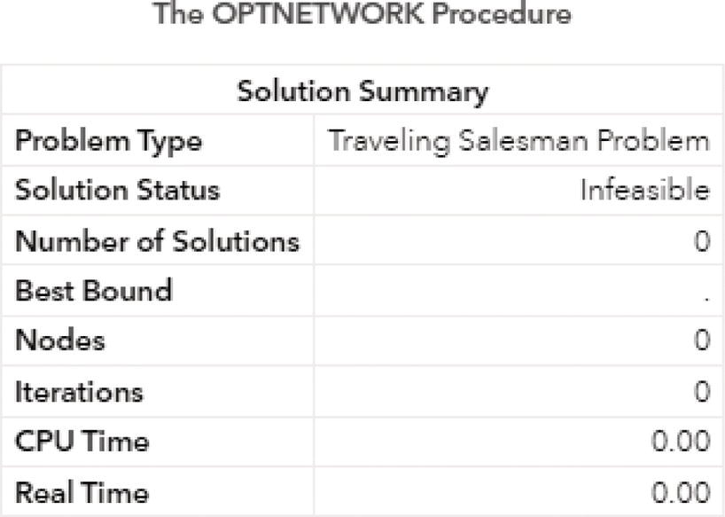
Figure 4.114 Output results by proc optnetwork running the traveling salesman algorithm based on a directed input graph with the link ( A , H , 3).
VRP in real‐world applications can be complex involving factors like the number and locations of all possible stops on the routes, arrival and departure time gaps, effective loading, vehicle limitations, time windows, loading process at depots, multiple trips, inventory limitations, multiples depots where vehicles can start and end, among others. The list of possible constraints is practically endless.
In proc optnetwork, the VRP finds a set of elementary cycles in an input graph G = (N ′ L) that start and end at a common node, visit all other nodes once, and satisfy the vehicle capacity limits at the minimum cost. Usually in the VRP, the referred common node is a depot, and the referred all other nodes are the customers. The node set N = C ∪ {1} consists of a set of customer nodes (C) and a depot node (1). A route is an elementary cycle that starts and ends at the depot node. A route is serviced by a vehicle that picks up goods at the depot node and delivers them to its assigned set of customer nodes. Each customer has a demand d i , and each vehicle has a capacity Q. The number of routes (K) that are used by the vehicle varies depending on the vehicle fleet configuration. The number of routes is restricted to be greater than or equal to a lower limit K l and less than or equal to an upper limit K u .
Each link i, j ∈ L in the VRP is associated with a binary variable x e . Similar to the TSP, this binary variable indicates whether or not the link i, j is part of the recommended routes. Each link i, j is also associated with a continuous variable c ij . This variable indicates the weight of the link, or the cost to travel throughout that link. In addition to the variables associated with the links, an integer variable K indicates the number of routes to be used by the vehicle when traveling through the customer nodes.
An integer linear programming formulation of the VRP for a directed input graph G can be formulated as follows:

where for each subset S of customer nodes, δ(S) represents the set of links (i, j), with i ∈ S and j ∉ S. ![]() represents the set of outgoing links that are connected from node i and
represents the set of outgoing links that are connected from node i and ![]() represents the set of incoming links that are connected to node i.
represents the set of incoming links that are connected to node i.  represents a lower bound on the number of vehicles needed in order to service the set of customers S.
The first equation represents the leave node. The second equation represents the enter node. Both equations together ensure that each customer node is visited once and only once during the cycle. The third equation represents the leave depot. The fourth equation represents the enter depot. Both equations together ensure that the depot node is visited K times, once for each route. The last and fifth equation represents the capacity and the subtour. These inequalities enforce connectivity throughout the cycle and ensure that the vehicle capacity restriction is observed.
In the context of network flow, we can think of the VRP as a package delivery system where each node is a customer located in some particular geographic location, that demands a certain quantity of goods, and each link is a road that connects all those geographic locations. The goods need to be sent out from the depot node (which can be a central warehouse), must be loaded into the servicing vehicles, which have a limit capacity to transport the goods, and must be delivered to all the customers in the least amount of time, or by traveling the shortest distance, or producing the lowest cost.
In proc optnetwork, the VRP statement invokes the algorithm that solves the VRP. This algorithm is based on a variant of the branch‐and‐cut process described by Jens Lysgaard, Adam N. Letchford, and Richard W. Eglese in the paper “A New Branch‐and‐Cut Algorithm for the Capacitated Vehicle Routing Problem,” published in 2003 in the Mathematical Programming Journal. The VRP solver uses internally modified versions of two open‐source packages. In order to generate primal feasible solutions, proc optnetwork uses the package VRPH. To generate cutting planes to improve the dual bound, proc optnetwork uses the package CVRPSEP.
Similar to the TSP, there are many options for the VRP algorithm in proc optnetwork. Most of the algorithms in network optimization aims to minimize an objective function, which can be assigned to reduce time, distance, or cost within paths or cycles. The time, distance, or cost are commonly assigned to the link weight. Therefore, it is important in network optimization algorithms to properly define the link weight and specify it in proc optnetwork. The option WEIGHT= in the LINKSVAR statement is used to specify the time, distance, or the cost of the links in the input graph. This link weight is used by proc optnetwork when searching for the minimum cost routes associated with the VRP. If the link weight is not specified by using the WEIGHT= option, proc optnetwork will assume all links have the weight equal to 1.
Particularly for the VRP, the nodes definition is quite important. The nodes dataset defines the customer nodes and the demand they have for delivering goods. The option NODES= in PROC OPTNETWORK statement specifies the nodes data table containing the customers and their demands. The NODESVAR statement is used to specify the demand of the customer node by using the option LOWER=. If the customer node demand is not specified by using the LOWER= option, or it is missing in the nodes dataset, proc optnetwork will assume the customer demand is equal to 0. If the depot node is included in the nodes dataset, and has a demand associated, proc optnetwork will ignore the demand for the depot node.
Another important aspect is the direction of the graph, or the direction of the link within the input graph. As we noticed in the TSP, the same link set can produce a feasible or infeasible solution depending on the direction of the input graph. Again, undirected graphs create more possible paths between the customers nodes and the depot node, allowing more possible routes within the network. Directed graphs have less paths within the network as the direction of the link may progress or interrupt a particular route. Proc optnetwork can compute the VRP for both directed and undirected graphs. The option DIRECTION= defines the direction of the links within the network. Analogous to the TSP, if we create a links dataset for the VRP considering the direction of the link, in a directed graph, the from node will be the origin of the path and the to node will be the destination of that path. The exact same links dataset defined as undirected, both from and the to nodes can work as origin and destination. A link A → B is solely A → B in a directed graph as it can be A → B and B → A in an undirected graph.
The final result for the VRP algorithm in proc optnetwork is reported and saved in the output tables defined by the options OUT= and OUTNODES=. The output table specified in the OUT= option in the VRP statement reports the optimal routes as a sequence of links. This output table contains the following variables. The variable route that contains the route identifier, the variable route_order that contains the order or the sequence of the link within the route, the variable from that contains the origin node label of the link within the route, the variable to that contains the destination node label of the link within the route, and finally the variable weight that contains the cost of the link within the route. The cost can be anything around distance, time, price, or whatever variable that indicates the cost to travel through that link. The output table specified in the OUTNODES= option in the PROC OPTNETWORK statement reports the optimal route as a sequence of nodes. This output table contains the following variables. The variable node contains the node label, and the variable demand that contains the customer demand, the variable route that contains the identification of that particular route, and finally the variable route_order contains the order or the sequence of the node in the optimal route.
The option ABSOBJGAP= or ABSOLUTEOBJECTIVEGAP= specifies a stopping criterion for the algorithm when searching for optimal routes. If the absolute difference between the best integer objective and the objective of the best remaining branch‐and‐bound node becomes less than the value specified in the option, the solver stops searching for more solutions. The value of number specified in the option can be any nonnegative number. The default value is 0.000001.
The option RELOBJGAP= or RELATIVEOBJECTIVEGAP= specifies a stopping criterion for the algorithm when searching for optimal routes. This stopping criterion is based on the best integer objective and the objective of the best remaining node. The relative objective gap is the difference between the best integer objective and the objective of the best remaining node divided by the objective of the best remaining node. When the relative objective gap becomes less than the number specified in the option, the solver stops searching for an optimal solution. The value of number can be any nonnegative number. By default, the option RELOBJGAP= is set to 0.0001.
The option TARGET= specifies a stopping criterion for minimization problems. If the best integer objective is less than or equal to the number specified in the option, the solver stops searching for optimal routes. The value of the number specified in the option can be any number. The default is the largest negative number in magnitude that can be represented by a double.
The option CUTOFF= specifies the cutoff value for any branch‐and‐bound nodes in a minimization problem. The main idea of the cutoff is the following. If the optimal linear programming relaxation objective is not better than the cutoff value specified, then any mixed integer programming solution of a descendant can be no better than the cutoff. Then the node in the branch‐and‐bond method can be fathomed and does not need to be further considered in the search. If the objective value is greater than or equal to the number specified in the option, the algorithm stops the branch‐and‐bound search. The default is the largest number that can be represented by a double.
The option CUTSTRATEGY= specifies the level of mixed integer linear programming cutting planes to be generated. The cutting plane method iteratively refines the feasible set of solution values or the objective function by means of linear inequalities, also called cuts. This method is commonly used to find integer or mixed integer solutions in linear programming. The cutting plane method works by solving a non‐integer linear program by using a linear relaxation of the given integer program. Specific cutting planes are always generated by proc optnetwork when searching for optimal routes within input graphs. There are four options for the cutting strategy in proc optnetwork. The option AUTOMATIC generates cutting planes on the basis of a strategy that is determined by the mixed integer linear programming solver. The option NONE disables the generation of mixed integer linear programming cutting planes (some TSP‐specific cutting planes are still active for validity). The option MODERATE uses a moderate cutting strategy. Finally, the option AGGRESSIVE uses an aggressive cutting strategy. By default, proc optnetwork disables the generation of mixed integer linear programming cutting planes by using the option CUTSTRATEGY= NONE.
The option HEURISTICS= determines how frequently to apply primal heuristics during the branch‐and‐bound tree search. The application of primal heuristics to improve algorithm efficiency affects the maximum number of iterations that are allowed in iterative heuristics. Some computationally expensive heuristics might be disabled by the solver at less aggressive levels. There are five levels of how frequent proc optnetwork applies primal heuristics during the tree search. The option AUTOMATIC applies the default level of heuristics. The option NONE disables all primal heuristics. The option BASIC applies basic primal heuristics at low frequency. The option MODERATE applies most primal heuristics at moderate frequency. Finally, the option AGGRESSIVE applies all primal heuristics at high frequency. By default, the level of primal heuristics application in the tree search is AUTOMATIC.
The option LOGFREQ= or LOGFREQUENCY= specifies the time interval in seconds for printing information in the node log during the branch‐and‐bound algorithm. The node indicates the sequence number of the current node in the search tree. The number specified in the option can be any integer greater than or equal to zero. If the option is specified as 0, the node log is disabled. If the option is specified with any number greater than 0, the root node processing information is printed and, if possible, an entry is made at every number of seconds specified in the option. An entry is also made each time a better integer solution is found. By default, the option LOGFREQ= is specified at 5, which means printing information in the node log at every five seconds.
The option CAPACITY= specifies the capacity of each vehicle in the VRP. The capacity is the maximum amount of goods that a particular vehicle can pick up from the depot node and deliver to the customer nodes. The value specified in the option can be any nonnegative number. The default is the largest number that can be represented by a double. That means, if the capacity is not specified, proc optnetwork assumes unlimited capacity for a vehicle to collect goods from the depot nodes and deliver to the customers nodes.
The option DEPOT= specifies the depot node for the VRP. The centralized depot node is the source of all possible goods that will be delivered to the customer nodes. The value specified in the option must be present as a node within the links dataset. This option is required for the VRP because the depot node must be specified.
The option MAXROUTES= specifies the maximum number of routes allowed to service the overall customer’s demand. The value specified in the option must be an integer greater than or equal to 1. The default value is the largest number that can be represented by a 32‐bit integer.
One the other hand, the option MINROUTES= specifies the minimum number of routes allowed to service the overall customers demand. The value of number must be an integer greater than or equal to 1. By default, the value of the minimum number of routes allowed equals to 1.
The option MAXNODES= specifies the maximum number of branch‐and‐bound nodes to be processed. The default is any nonnegative integer that can be represented by a 32‐bit integer. When running the mixed integer liner programming in concurrent mode, the solver stops as soon as the number specified in the option is reached on any machine. When running the mixed integer linear programming algorithm in distributed mode, the solver periodically checks the total number of nodes that are processed by all grids and stops when the number specified in the option is reached.
The option MAXSOLS= specifies a stopping criterion. When the number of solutions specified in the option is found, the procedure stops searching for new optimal solutions. The default is the largest number that can be represented by a 32‐bit integer.
The option MAXTIME= specifies the maximum amount of time to spend solving the TSP. The type of time can be either CPU time or real‐time, and is determined by the value of the TIMETYPE= option in the proc optnetwork statement. The default is the largest number that can be represented by a double. The maximum time limits the optimization process, including the problem generation and the solution time. If the MAXTIME= option is not used, the solver does not stop based on the amount of time elapsed during the optimization process.
The option MILP= specifies the type of algorithm proc optnetwork uses to find the optimal TSP tour. Proc optnetwork might or might not use a mixed integer linear programming solvert. The mixed integer linear programming solver attempts to find the overall best tour by using the branch‐and‐cut algorithm. This algorithm can be very expensive for large‐scale problems. The value TRUE in the option MILP= specifies the mixed integer linear programming solver as the algorithm used by proc optnetwork. The option FALSE determines proc optnetwork to use its initial heuristics to find a feasible, but not necessarily optimal tour, as quickly as possible. By default, proc optnetwork uses the mixed integer linear programming approach based on the branch‐and‐cut algorithm (option MILP = TRUE).
4.13.1 Finding the Optimal Vehicle Routes for a Delivery Problem
Let's use a network flow graph to demonstrate the VRP using proc optnetwork. The graph presented in Figure 4.115 shows a network with 8 nodes and only 17 links. From the set of nodes, node X is the depot node. All the other 7 nodes, A, B, C, D, E, F, and G are the stores, or the customers. Each store or customer node also has a specific demand. Each link has a cost associated with flow the goods from the depot node to the store nodes. Initially, we assume this network as an undirected graph, which means, each link in the network has two directions, connecting nodes to outflow and inflow goods.
The following code describes how to create the input datasets for the VRP. The links dataset has the nodes identification, the from and to variables indicating origin and destination for the possible routes between depot and stores, as well as between stores. The cost for each link is also defined in the links dataset by weight variable. The nodes dataset has the stores or customer identification plus the demand of each node.
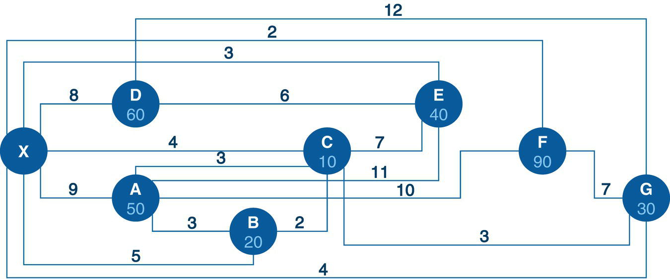
Figure 4.115 Undirected input graph with weighted links and nodes demands.
data mycas.links;input from $ to $ weight @@;datalines;X A 9 X B 5 X C 4 X D 8 X E 3 X F 2 X G 4 A B 3 A C 3A E 11 A F 10 B C 2 C E 7 C G 3 D E 6 D G 12 F G 7;run;data mycas.nodes;input node $ demand @@;datalines;A 50 B 20 C 10 D 60 E 40 F 90 G 30;run;
Once the links and nodes datasets are created, defining possible routes with costs, and stores with demands, we can invoke the VRP algorithm in proc optnetwork to solve the VRP. The following code describes how to do that. The links definition using the LINKSVAR statement specifies the variables from and to as the origin and destination for all possible routes within the network. The variable weight specifies the cost to flow goods throughout those possible routes. The input graph in this example is defined as an undirected network. In that case, proc network creates two possible directions for each link, allowing outflow and inflow through the same link. For example, the first original link (X, A) turns into two distinct links (X, A) and (A, X) when proc optnetwork is solving the VRP. The nodes definition using the NODESVAR statement specifies the store node identification and the demand for each node, or how many product deliveries each store requires. The output table defined in the OUTNODES= option saves for each node in each route it will be served and in what order. The output table defined in the OUT= option within the VRP statement saves the routes and the order of the links that will be used in each route to deliver the goods to the store nodes. The DEPOT= option in the VRP statement defines the depot node in the VRP. The CAPACITY= option in the VRP statement defines the capacity of the vehicle when delivering the goods throughout the store nodes.
proc optnetworkdirection = undirectedlinks = mycas.linksnodes = mycas.nodesoutnodes = mycas.nodesout;linksvarfrom = fromto = toweight = weight;nodesvarnode = nodelower = demand;vrpdepot = Xcapacity = 100out = mycas.routes;run;
Figure 4.116 shows the output for the VRP algorithm. It shows the size of the input graph, 8 nodes and 17 links. It also states that an optimal solution was found (solution status is optimal), one single solution was found (number of solutions 1) and the objective value is 44, which represents the routing cost to deliver the demanded goods from the stores from the depot node.
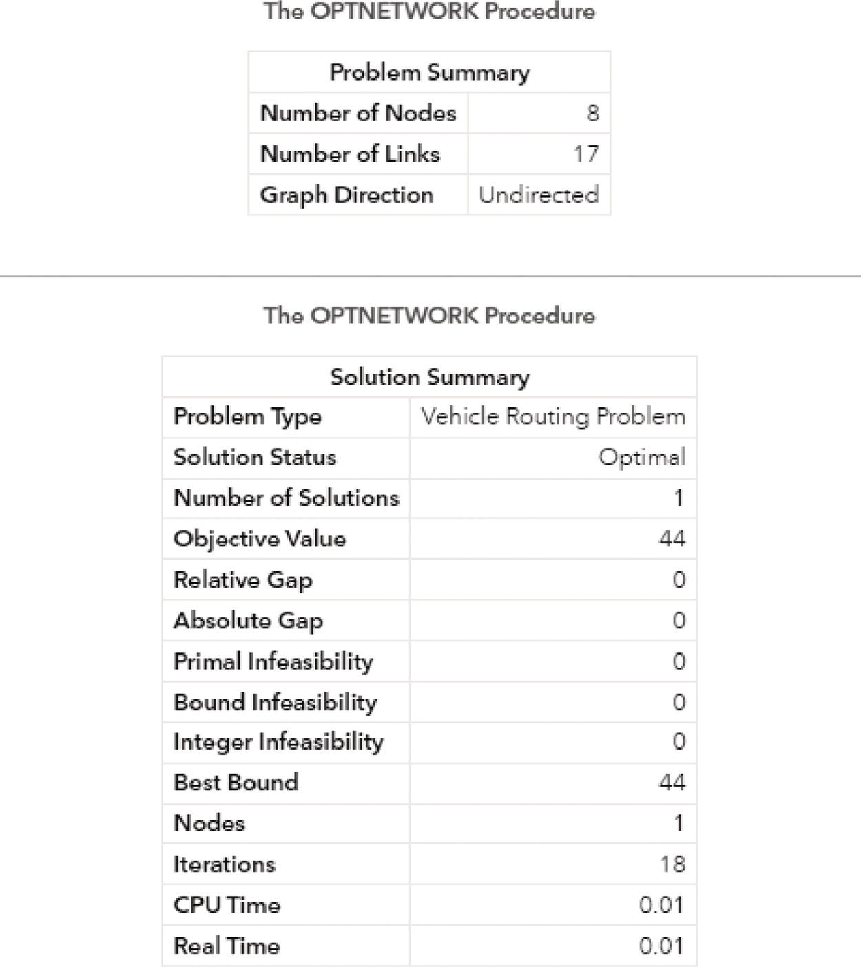
Figure 4.116 Output results by proc optnetwork running the vehicle routing problem algorithm based on an undirected input graph.
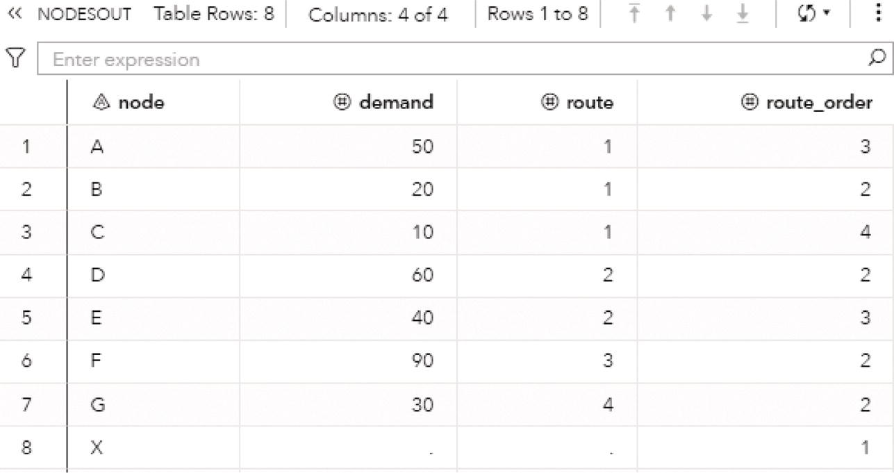
Figure 4.117 The set of store nodes and in which route and order they will be served in the vehicle routing problem solution based on an undirected graph.
The following pictures show the detailed results of the VRP generated by proc optnetwork. The NODESETOUT dataset presented in Figure 4.117 shows the variable node that identifies the node label, the variable demand, which specifies the demand for each store node, the variable route, which specifies what route will serve that store node, and the variable route_order, which specifies in what order of that route the store node will be served.
In this example, the store nodes A, B, and C will be served by route 1. The vehicle loads at the depot node X and departs to the store node B, delivering the 20 goods demanded. The order of the route is 2, as the first step (route_order 1) is at the depot node X. The vehicle then goes from the store node B to the store node A (route_order 3), delivering the 50 goods demanded, and finally serves the store node C (route_order 4) delivering the 10 goods demanded. After that, the vehicle returns to the depot node X to reload. Notice that the first route considers a total amount of goods as 80, 20 for node B, 50 for node A, and 10 for node C. As the capacity of the vehicle is 100, the vehicle cannot take any more goods to deliver to other store nodes. That is the reason it returns to the depot node X to reload and continues the delivering. It is important to notice here that the first loading process at the depot node X does not need to be the maximum capacity of the vehicle, 100. Based on the optimal routing, the vehicle will deliver only 80 goods throughout the 3 store nodes B, A, and C. The vehicle can therefore load only the 80 units required. The second route serves nodes D and E. At the depot node X, the vehicle reloads with 100 units. From the depot node X the vehicle goes to the store node D (route_order 2), delivering the 60 goods demanded. From store node D, the vehicle proceeds to the store node E (route_order 3) and deliver the 40 goods demanded. As these 2 store nodes demand a total of 100 units, the maximum capacity of the vehicle, the routing stops and the vehicle returns to the depot node X to reload. Now the vehicle reloads 90 units. From the depot node X, the vehicle goes to the store node F and delivers the 90 goods demanded. Due to the limit capacity of the vehicle, there are no more store nodes that can be served, and the route 3 has only one single stop (route_order 2 only). The vehicle goes once again to the depot node X to reload. Now it gets only 30 units, which is the demand of the last store node. The vehicle departs from the depot node X and goes to the store node G, delivering the 30 goods demanded. As node G is the last store node to be served, the route 4 has one single stop (route_order 2 only). As all store nodes are properly served, the vehicle can return to the depot node X, finalizing the routing.
The ROUTES dataset presented in Figure 4.118 shows the variable route that specifies the route taken by the vehicle to serve the store nodes, the variable route_order that specifies the order of the route when the vehicle deliver the goods to the store nodes, the variables from and to that represent the link taken by the vehicle at each step of the route, and finally the variable weight that represents the cost for taking that link.
Similar to the previous output, the ROUTES dataset shows the routes and the order of the links taken by the vehicle in order to serve all the store nodes within the network. Route 1 comprises 4 links. From the depot node X to the store node B, then from the store node B to the store node A (notice here that proc optnetwork uses the original link definition (A, B) from the links dataset, even though the direction for this link in the route is from B to A), from the store node A to the store node C, and finally from the store node C to the depot node X. Similarly, proc optnetwork uses the original link (X, C) from the links dataset, even though the direction of this link in the route is from C to X). The total cost for this route is 15, considering all the links (X, B, 5), (A, B, 3), (A, C, 3), and (X, C, 4). The route 2 comprises 3 links, from the depot node X to the store node D, then from the store node D to the store node E, and finally from the store node E back to the depot node X. The total cost of this route is 17, considering the links (X, D, 8), (D, E, 6,) and (X, E, 3). Route 3 has 2 links, from the depot node X to the store node F, and then from the store node F back to the depot node X. The total cost of this route is 4, with the links (X, F, 2) and (X, F, 2). Finally, route 4 has also just 2 links, from depot node X to store node G and then back to depot node X. The total cost of this route is 8, with the links (X, G, 4) and (X, G, 4). The overall cost for the VRP is 44, as stated before, considering all 4 routes with individual costs at 15, 17, 4, and 8, respectively.
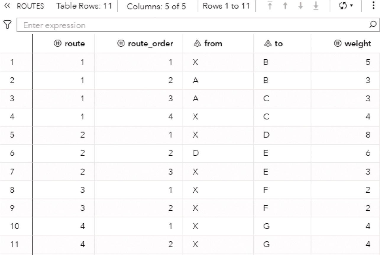
Figure 4.118 The order of the links for each route in the vehicle routing problem based on an undirected graph.
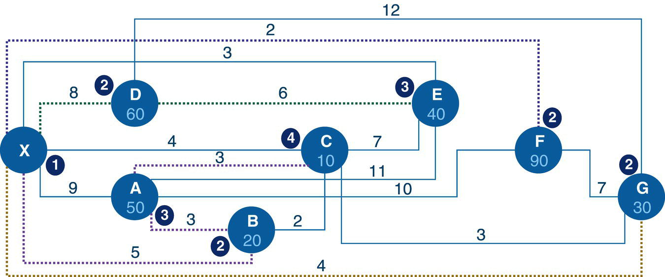
Figure 4.119 The vehicle routing problem solution generated by proc optnetwork based on an undirected graph.
Figure 4.119 shows a possible solution for the VRP considering the input graph.
When we look at the network flow diagram, we can probably visualize that the first route would be something like, from the depot node X to the store node A, then from the store node A to the store node B, from the store node B to the store node C and finally from the store node C back to the depot node X. The total cost of this route would be 9 (X, A, 9) plus 3 (A, B, 3) plus 2 (B, C, 2) plus 4 (C, X, 4), which sums up to 16. Proc optnetwork searches for the minimum cost for all routes within the VRP. The optimal route in volving nodes X, A, B and C is indeed X → B → A → C → X, with a total cost of 15 (instead of 16), as 5 (X, B, 5) plus 3 (B, A, 3) plus 3 (A, C, 3) plus 4 (C, X, 4).
The VRP solution provided by proc optnetwork for this small example found four distinct routings to deliver goods to all store nodes and meet the supply demands. This solution can be accomplished by using 1 single vehicle, going around three times in a sequence. For example, load at depot node X, deliver goods to the customer nodes A, B, and C, return to the depot node X to reload, deliver goods to the customer nodes D and E, return to the depot node X to reload, deliver goods to the customer node F, return to the depot node X to reload, deliver goods to the last customer node G, and finally return to the depot node X. This solution can also be accomplished by using four different vehicles. The first vehicle takes the routing for customer nodes A, B, and C, the second vehicle takes the routing for customer nodes D and E, the third vehicle takes the routing for customer node F, and the fourth vehicle takes the routing for customer node G. Of course, this solution can also be accomplished by using two or three vehicles, splitting the routings among them, and supplying the customers' demands by using the found routings in parallel.
Key information in the VRP though is the capacity of the vehicle. It changes the solution completely found by proc optnetwork. To lower the capacity, requires more trips the vehicle needs to perform to supply all the customer nodes demands. Depending on how low the maximum capacity of the vehicle is, the solution for the VRP can be infeasible, as the vehicle cannot deliver the units demanded by a particular customer node. Of course, the vehicle could make multiple trips to the same customer node until the demand is supplied, but this option is not considered by proc optnetwork. On the other hand, the higher the maximum capacity of the vehicle, the fewer trips the vehicle needs to perform to deliver all goods and fulfill the customer nodes demands. For example, an unlimited capacity for an imaginary vehicle would allow one single trip to deliver all goods to all customer nodes demands.
Let's take a look at how these options work in practice when using proc optnetwork to solve the VRP. First, we’ll check on the first lower boundary extreme. The following code defines the maximum capacity for the vehicle as 89:
proc optnetworkdirection = undirectedlinks = mycas.linksnodes = mycas.nodesoutnodes = mycas.nodesout;linksvarfrom = fromto = toweight = weight;nodesvarnode = nodelower = demand;vrpdepot = Xcapacity = 89out = mycas.routes;run;
As the store node F has a demand of 90, the vehicle defined with a maximum capacity of 89 cannot deliver enough units at once to the store node F and the solution is infeasible. Figure 4.120 shows the summary result reported by proc optnetwork with the infeasible solution.
Now let's go to the other extreme and make the maximum capacity of the vehicle much higher. The following code increases the maximum capacity for the vehicle to 500:
proc optnetworkdirection = directedlinks = mycas.linksnodes = mycas.nodesoutNodes = mycas.nodesout;nodesVarnode = nodelower = demand;linksvarfrom = fromto = toweight = weight;vrpdepot = 'X'capacity = 500out = mycas.routes;run;
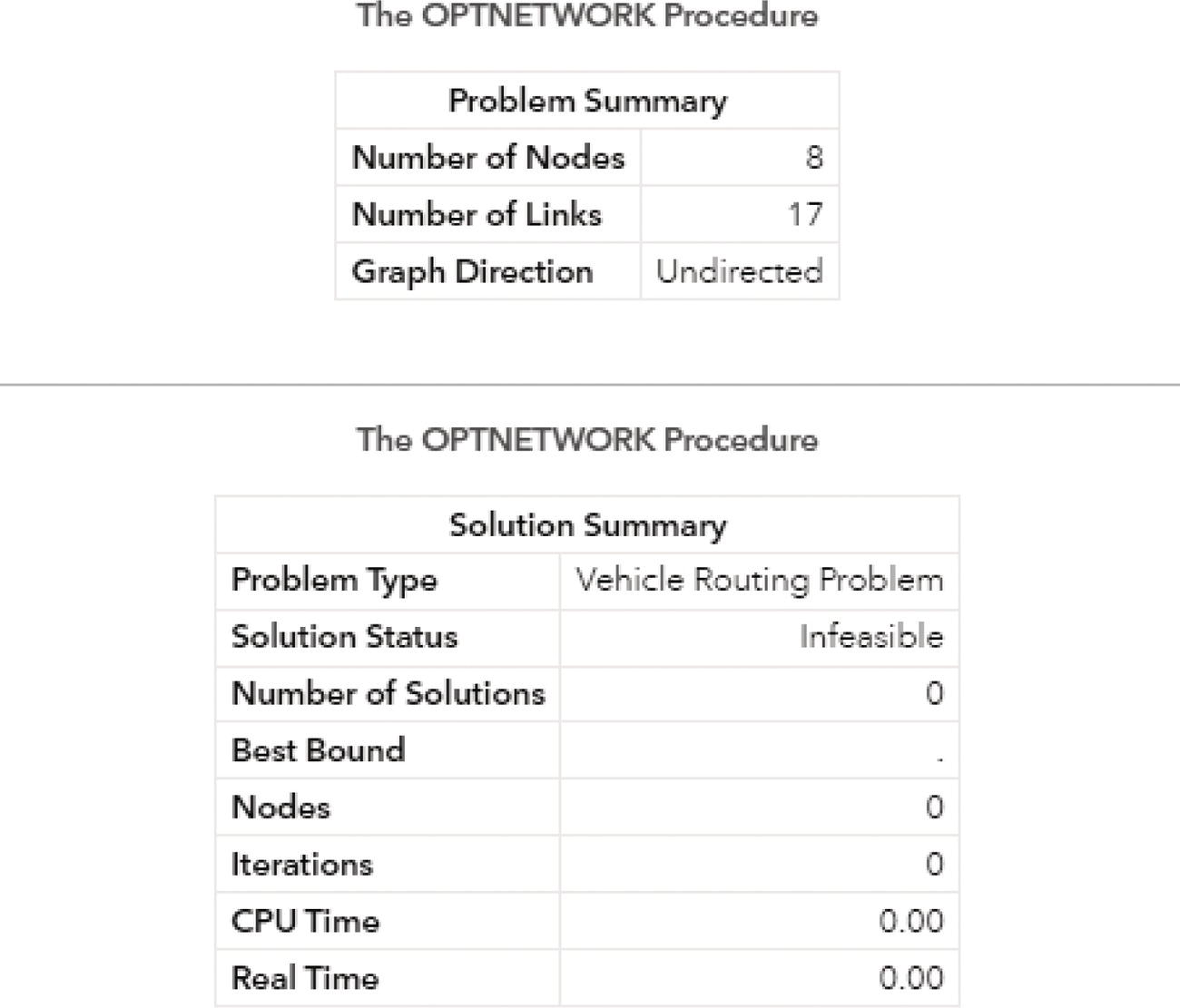
Figure 4.120 The infeasible solution for the vehicle routing problem when using a low maximum capacity for the vehicle.
A vehicle with a maximum capacity of 500 units makes an optimal solution for the VRP possible. The outputs from proc optnetwork are shown in the following pictures. Two optimal solutions were found by proc optnetwork, and the total cost of the optimal routing is 39. Figure 4.121 shows the summary result reported by proc optnetwork with the optimal solution.
The NODESETOUT dataset presented in Figure 4.122 shows the depot node X and all store nodes, including the chosen routes and the orders within the routes.
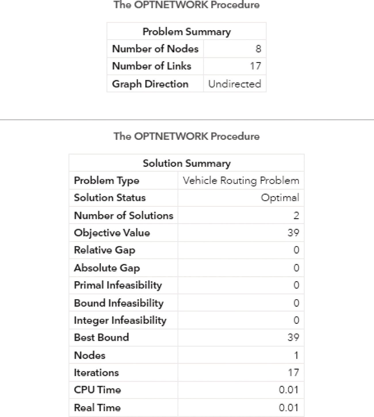
Figure 4.121 The feasible solution for the vehicle routing problem when using a high maximum capacity for the vehicle.
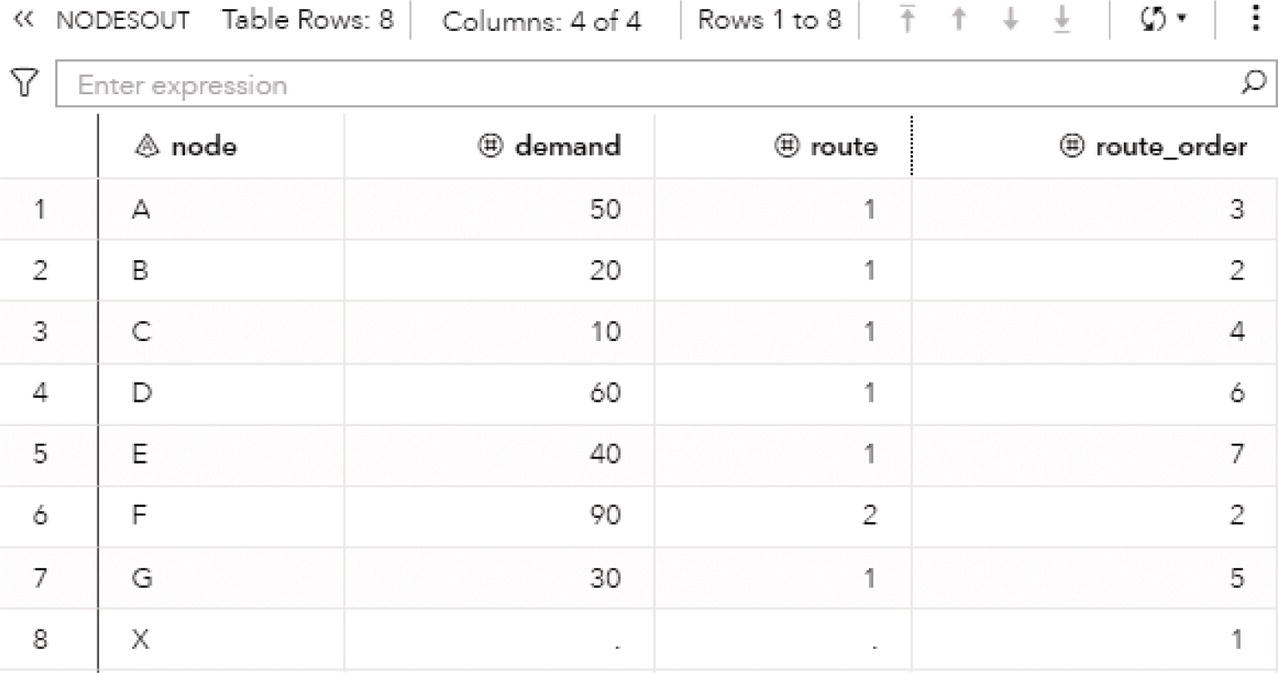
Figure 4.122 The set of nodes and the demands.
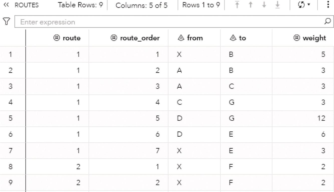
Figure 4.123 The routes and the sequence of nodes.
The total demand considering all 7 store nodes are 300 units. Notice that even though the vehicle maximum capacity is 500 units, there are still 2 routes to supply the goods to all the store nodes. The ROUTES dataset presented in Figure 4.123 shows the routes.
The constraint here though is not the maximum capacity of the vehicle but the existing links within the network and its weights. In the optimal route, the vehicle departs from depot node X and covers the store nodes B, A, C, G, D, and E in one single route, returning to the depot node X with a total cost of 35. The vehicle then departs from the depot node X and goes to the store node E and returns to the depot node X in a single trip with a total cost of 4. The overall cost of the VRP is 39. The vehicle could take a route to go over all the store nodes without stopping at the depot node X to resume the delivering process. For example, the vehicle can go from X to B, A, C, E, D, G, F, and then back to X. The total cost for this route is 45 (5 + 3 + 3 + 7 + 6 + 12 + 7 + 2). The minimum cost to cover all the store nodes is indeed by returning at some point to the depot node X and resuming the route. If we consider that the paths from the store node E to the depot node X, from the depot node X to the store node F, and then back to the depot node X are just existing links, we would have just one single route. However, if we consider that there is a cost associated with carrying over the goods in the vehicle, we can make the overall route in 2 steps. Instead of making the vehicle depart from the depot node X with all 300 units, we can make it depart with only 210 units to deliver the goods to B, A, C, G, D, and E. As the vehicle needs to pass by the depot node X to minimize the cost of the trip, it can stop by and reload with the additional 90 units to serve the store node F. That is the reason proc optnetwork considers the overall vehicle routing with 2 routes, as the vehicle needs to go back to the depot node X to proceed in the minimum cost path. If there was a link between E and F with a low‐cost weight, for example, 2, the minimum cost path would likely be X, B, A, C, G, F, E, D, X, with total cost at 37. The vehicle wouldn't need to pass by the depot node X at any time but to start and end the routing.
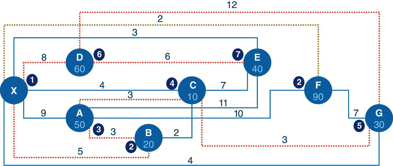
Figure 4.124 The vehicle routing problem solution with a high vehicle maximum capacity.
Figure 4.124 shows the solution considering the maximum capacity for the vehicle as 500 units.
Now, let's consider the network as a directed graph. A directed graph completely changes the existing links within the network and of course, changes the possible solutions found by proc optnetwork in the VRP.
The exact same network as a direct graph is shown in Figure 4.125.
Using the same links and nodes dataset definitions, we have a directed graph with 17 links and 8 nodes. The following code invokes the VRP algorithm to run on a directed graph.
proc optnetworkdirection = directedlinks = mycas.linksnodes = mycas.nodesoutnodes = mycas.nodesout;linksvarfrom = fromto = toweight = weight;nodesvarnode = nodelower = demand;vrpdepot = 'X'capacity = 500out = mycas.routes;run;
The output from the proc optnetwork shows that there is no feasible solution for this problem, considering there is no sufficient existing links to allow the vehicle to depart from the depot node X and cover all the store nodes in this particular directed network. Figure 4.126 shows the summary result reported by proc optnetwork with the infeasible solution for the directed graph.
Based on the links definition, there are no links returning to the depot node X. That makes the solution infeasible. Then, let's add some links from the store nodes to the depot node X. The following code adds another 3 links to the network, creating possible paths from the store nodes E, F and G to the depot node X.
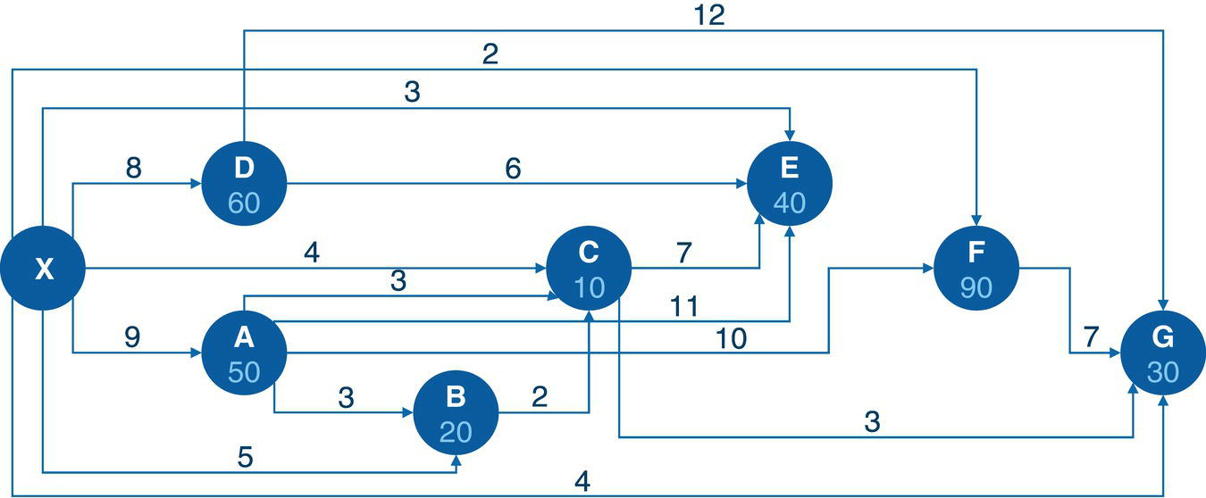
Figure 4.125 The vehicle routing problem based on a directed graph.
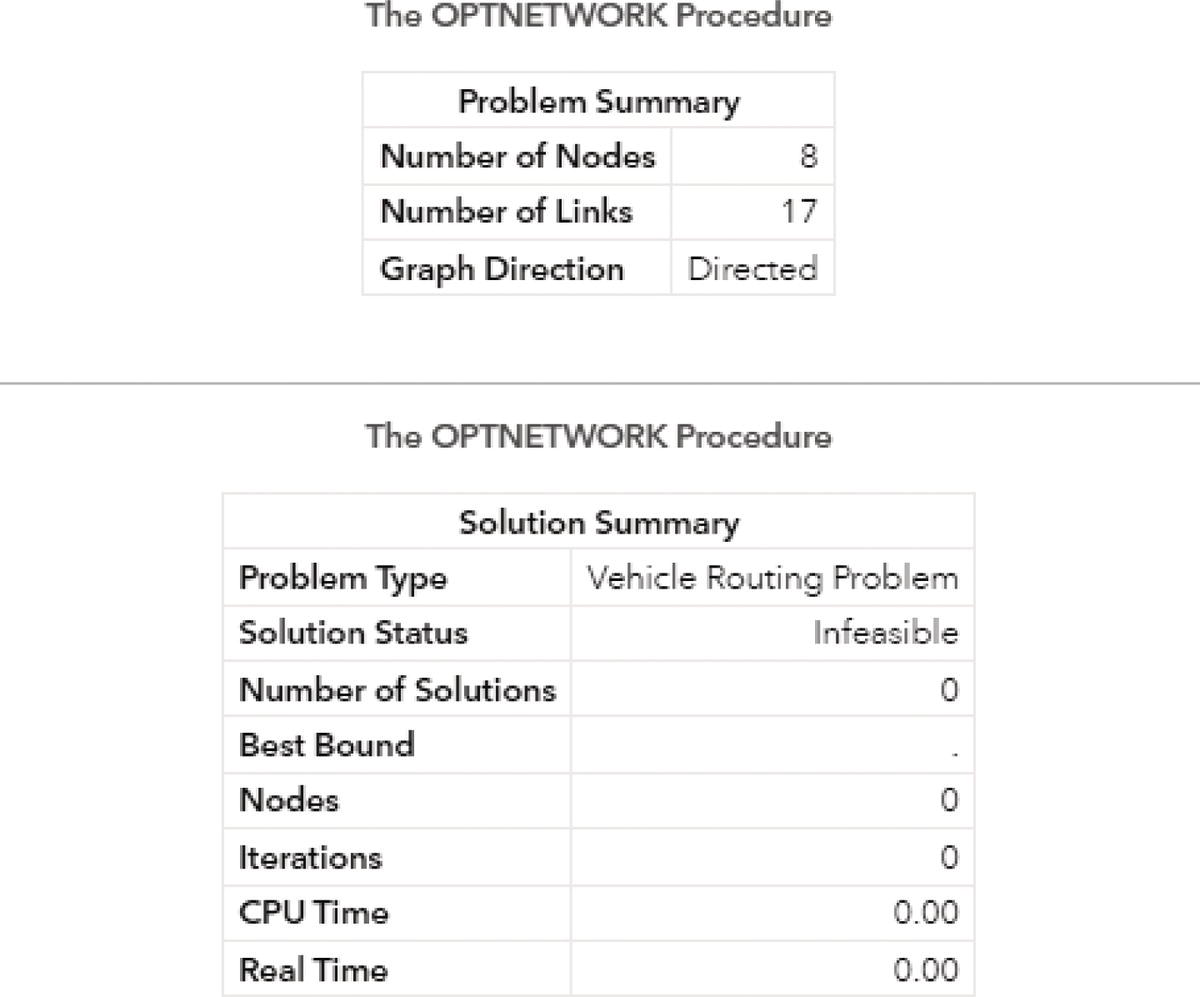
Figure 4.126 The solution for the vehicle routing problem with a high vehicle maximum capacity.
data mycas.links;input from $ to $ weight @@;datalines;X A 9 X B 5 X C 4 X D 8 X E 3 X F 2 X G 4 A B 3 A C 3A E 11 A F 10 B C 2 C E 7 C G 3 D E 6 D G 12 F G 7G X 8 F X 12 E X 15;run;
The new directed graph is presented in Figure 4.127.
There are now possible paths to return the vehicle to the depot node X, from the store nodes E, F, and G. We can rerun the exact same code shown previously to invoke the VRP algorithm in proc optnetwork to search for an optimal solution based on this new directed graph.
The outputs from proc optnetwork are shown in the following pictures. Figure 4.128 shows that one optimal solution was found by proc optnetwork and the total cost of the optimal routing is 68.
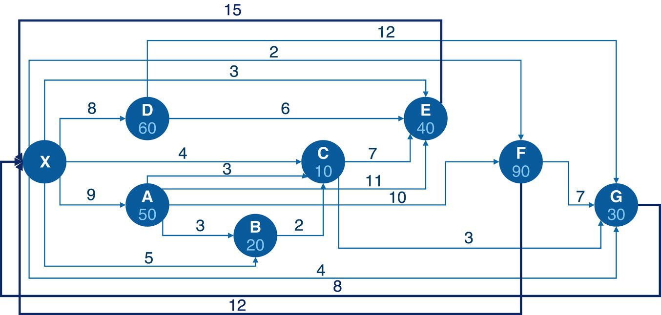
Figure 4.127 The vehicle routing problem based on a directed graph with additional links to the depot node.

Figure 4.128 The feasible solution for the vehicle routing problem based on a directed graph.
The NODESETOUT dataset presented in Figure 4.129 shows the depot node X and all the store nodes, including routes and the sequence of nodes within the routes.
There are three routes considered by the optimal solution. The first route serves the store nodes A, B, C, and G, supplying 50, 20, 10, and 30 units of demand, respectively. The second route serves the store nodes D and E, supplying 60 and 40 units, respectively. Finally, the third route serves the store node F, supplying 90 units. The same concept applies here. It could be one single vehicle covering all the store nodes by doing three trips, or it could be three vehicles covering all the store nodes by doing one single trip each.
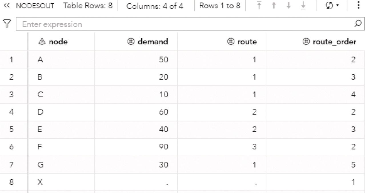
Figure 4.129 The set of nodes, the routes, and the sequence of nodes within the routes.
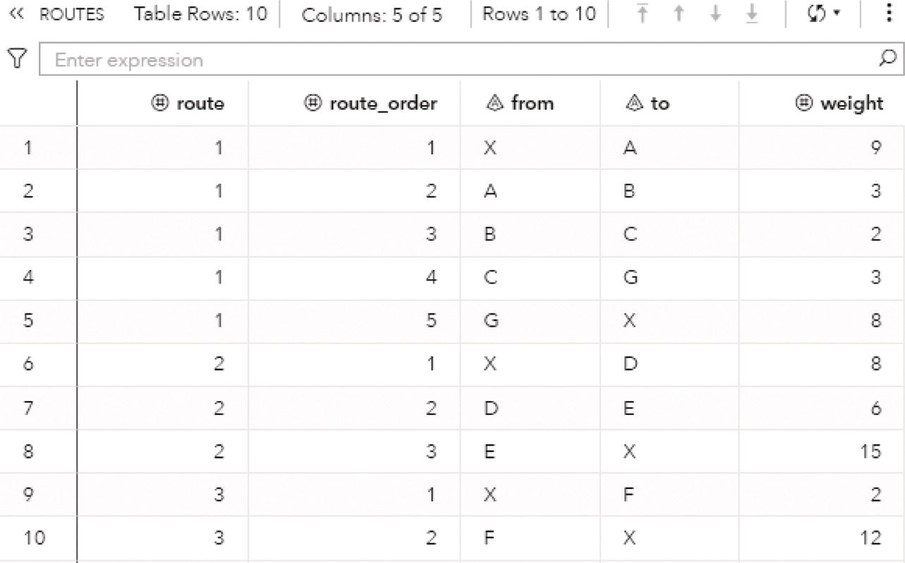
Figure 4.130 The routes and the sequence of nodes.
The ROUTES dataset presented in Figure 4.130 shows the routes and the sequence of links performed by the vehicle when delivering the goods to all the store nodes. For a directed graph, this output dataset is particularly important for the VRP solution because it shows the real links traveled by the vehicle, considering the actual direction of the links. Remember that for the undirected graph, even though we know that the vehicle goes from node B to node A in the optimal routing solution, the link presented in the output dataset is the link (A, B, 3), because this is the original link defined in the links dataset.
The vehicle loads 110 units in the depot node X. It goes to the store node A and delivers 50 units at the cost of 9 (X, A, 9). Then the vehicle goes to the store node B and delivers 20 units at the cost of 3 (A, B, 3). It progresses on the routing and goes to the store node C and delivers 10 units, at the cost of 2 (B, C, 2). Finally, the vehicle goes to the store node D and delivers the last 30 units, at the cost of 3 (C, G, 3). The vehicle then returns to the depot node X at the cost of 8 (G, X, 8). The total cost for this route is 25. On the second trip, the vehicle loads 100 units at the depot node X and departs for the store node D, delivering 60 units at the cost of 8. (X, D, 8). Then the vehicle goes to the store node E and delivers 40 units at the cost of 6 (D, E, 6). The vehicle then returns to the depot node X at the cost of 15 (E, X, 15). The total cost for this route is 29. Finally, the vehicle loads 90 units and goes straight to the store node F, delivering those goods at the cost of 2 (X, F, 2). The vehicle then returns to the depot node X at the cost of 12 (F, X, 12). This route has a total cost of 14. The overall cost for the optimal solution is 68 (25 + 29 + 14).
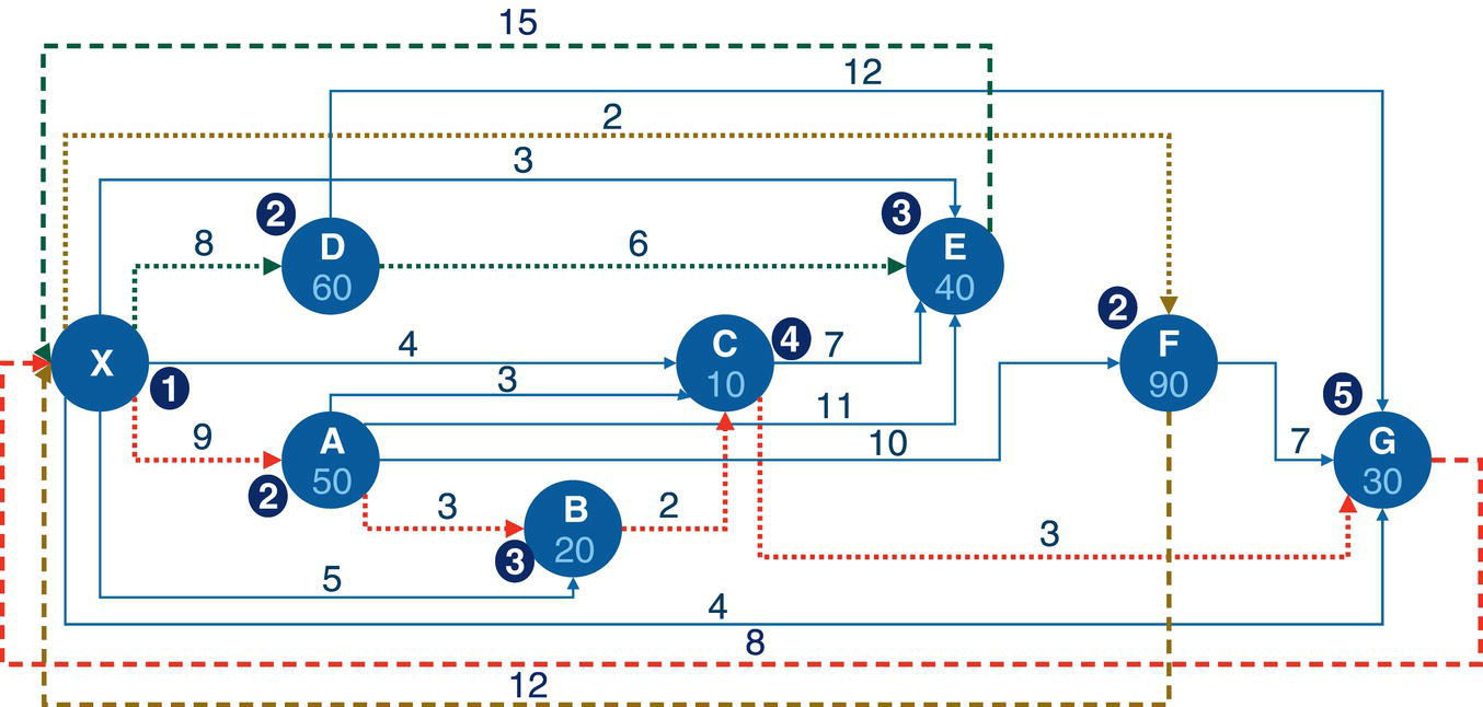
Figure 4.131 The vehicle routing problem solution based on a directed graph.
Figure 4.131 shows the optimal solution considering the directed graph.
Once again, the same concepts of multiple vehicles and multiple trips applies to the directed graph. Most of the time, real‐world problems are based on directed graphs, as physical roads (streets, avenues, highways, etc.) not always having two‐way directions. Many real‐world problems in the VRP are much more complex than was described here. Those problems can include time window constraints, where the goods need to be delivered in a certain time frame. Deliveries out of the time window can incur penalties. Groceries delivered by the major supermarket chains represent real‐life scenarios like this. Other problems can involve pickup and delivery constraints. Routes need to be dynamically optimized allowing drivers to pick up and deliver goods. Food delivery companies represent real‐life scenarios like this. Capacity constraint is also common in real‐world problems. Multiple vehicles have different capacities, and these differences must be considered when optimizing the vehicles routings. Sometimes vehicles also have constraints on what they can transport, like heavy equipment, frozen food, delicate goods, etc.
As we can see, there are many variants and specializations of the VRP to address real‐world business problems. And to make matters worse, most of the life‐scenarios happen with a few combinations of the specializations described previously. The VRP includes manual solving and optimization solvers, sometimes working together with heuristics approaches to narrow down the number of possible solutions based on the size of the problem (depot/store/customer nodes, links/paths/routes, resources, constraints, etc.). The VRP is a field in optimization that continuously evolve, with many applications in different industries and businesses.
4.14 Topological Sort
A topological sort or topological ordering of a directed graph is a linear ordering of its nodes, where for every directed link (i, j) from node i to node j, node i comes before node j in that ordering. A classic example is when tasks are considered to be represented by a graph. Each node within the graph represents a task, and the links between the nodes represent some constraints associated with the order of the tasks. For example, in a brewing process, simplistically, the first step is the mashing process, the second step is the boiling process, and finally, the third step is the fermentation process. In a graph representation, mashing can be represented by node i, boiling can be represented by node j, and fermentation can be represented by node k. The links between the nodes can represent the sequence in which the tasks need to be performed. The mashing process needs to be completed before the boiling process starts. A directed link from node i to node j can represent that ordering. The fermentation process can only start after the boiling process is completed. Then, a directed link from node j to node k can represent that mandatory sequence. Figure 4.132 illustrates that sequence.
A simple directed graph to represent the tasks associated with the nodes i, j, and k, and the ordering between them is shown in Figure 4.133.
In this example, the topological sort is just a valid sequence for the tasks. Formally, a topological sort is a graph traversal in which each node n is visited only after all its dependencies are visited, or all other previous nodes are visited. A topological sort cannot happen if the directed graph has cycles. This property is commonly referred to as a directed acyclic graph, or simply DAG. Any DAG has at least one topological sort.
Figure 4.132 The first steps of the brewing process (USA Hops).

Figure 4.133 The directed graph representing task and their ordering.
The most common application of topological sort is to schedule a sequence of jobs or tasks based on their dependencies. The tasks are represented by nodes and the dependencies are represented by links. The directed link connecting the nodes defines the dependency or ordering of the tasks. The task in the origin node must be completed before the task in the destination node can be started. The topological sort gives the order in which tasks must be performed.
In proc optnetwork, the TOPOLOGICALSORT (or TOPSORT) statement invokes the algorithm that calculates a topological ordering of the nodes of a directed acyclic input graph.
The final result for the topological sort algorithm in proc optnetwork is reported and saved in an output table defined by the OUTNODES= option. The output table contains the variable node that identifies the node in the topological sort, and the variable top_order that identifies the order of the node in the topological sort.
4.14.1 Finding the Topological Sort in a Directed Graph
Let's consider the graph presented in Figure 4.134 to demonstrate the topological sort problem using proc optnetwork. The directed graph describes a network with just 8 nodes and only 10 links.
The following code describes how to create the input dataset for the topological sort scenario. A problem involving a topological sort requires only the links dataset. The links dataset represents both the tasks as origin and destination nodes, and the dependencies. The origin nodes represent the tasks that need to be performed and completed before the tasks represented by the destination nodes are executed. The links don't need to have weights as only the sequence of the nodes is taken into consideration when calculating the ordering of the topological sort.
data mycas.links;input from $ to $ @@;datalines;A B A C A D C B E B E F D F D H B G G H;run;
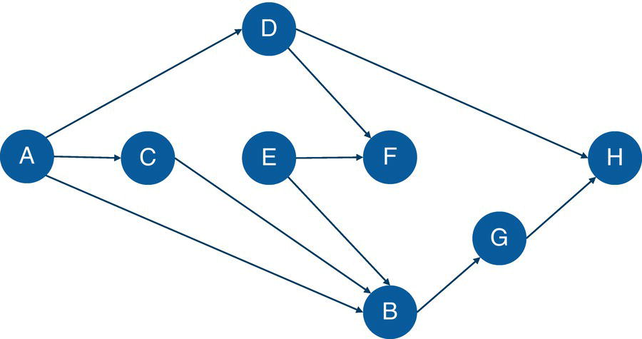
Figure 4.134 Input graph with directed links.
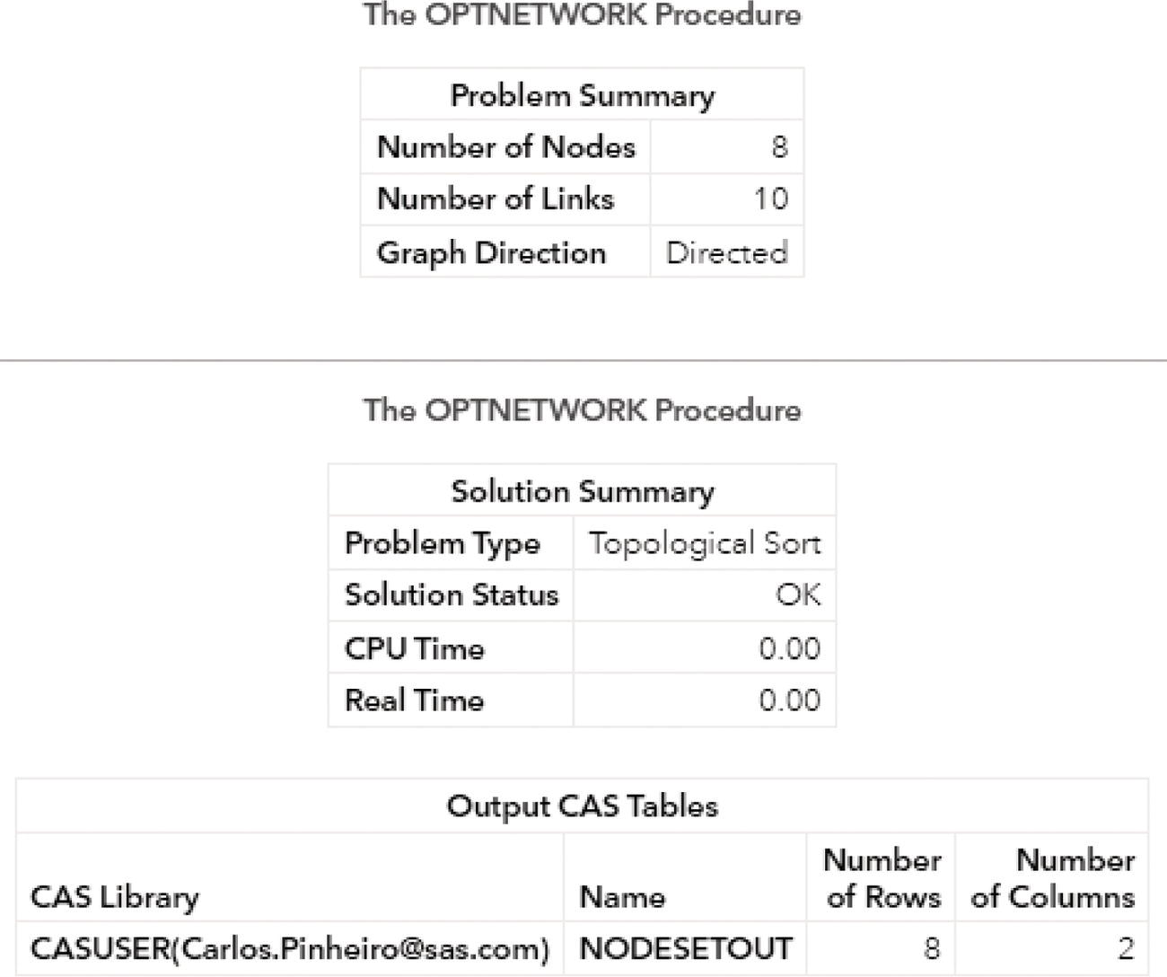
Figure 4.135 Output results by proc optnetwork running the topological sort algorithm.
Once the links dataset is created, we can now invoke the topological sort algorithm using proc optnetwork. The following code describes how to do it. The links are defined in proc optnetwork by using the LINKSVAR statement. No link weights are needed. Therefore, just the from and to variables are used to define origin and destination nodes in terms of dependencies. The network needs to be defined as a directed graph.
proc optnetworkdirection = directedlinks = mycas.linksoutnodes = mycas.nodesetout;linksvarfrom = fromto = to;topologicalsort;run;
Figure 4.135 shows the output for the topological sort algorithm. It says that a solution was found, as the solution status is ok.
Figure 4.136 presents the results for the topological sort problem. The OUTNODES dataset shows the variable node to identify the task, and the variable top_order to identify the order of the task in the topological sort.
Based on the solution provided by proc optnetwork, the task represented by the node E needs to be performed first. Then, the task represented by the node A can be executed. Following the task A, the task D can be performed. Then, the task F, the task C, the task B, then task G, and finally the task H. Figure 4.137 shows graphically the final solution in terms of the tasks ordering.
Notice that we can perform task A, and from there, execute tasks B, C, and D. Once task D is completed, we could perform task F. However, task F can only be executed when both tasks D and E are completed. Then, even if we execute task A, we still need to execute task E to run task F. For all other tasks, including G and H, task A is the predecessor. But again, there is no benefit to execute task A first, allowing all other tasks to be performed in a sequence, if task E is not completed. This is the reason that task E is the very first task in the topological sort.
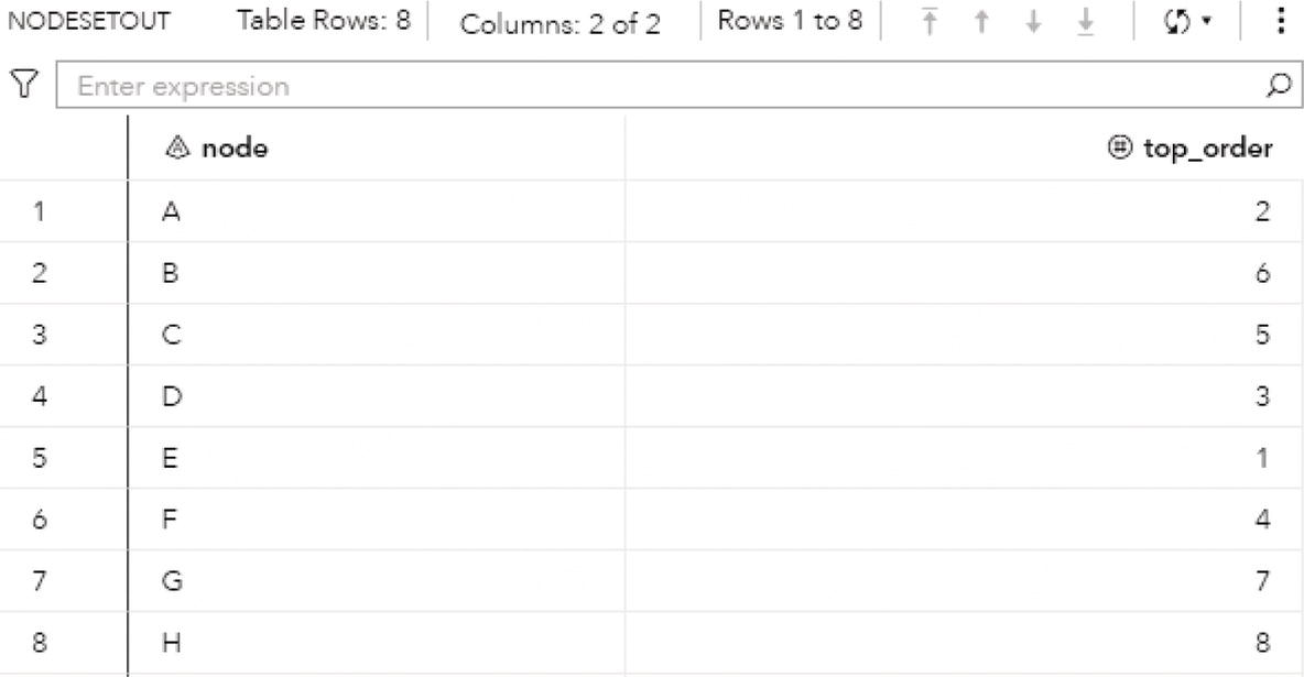
Figure 4.136 The topological sort solution.

Figure 4.137 Solution for the topological sort.
We can also think about the topological sort in terms of the terminal nodes, and then go backwards in the dependencies. In this example, we have 2 terminal nodes, tasks F and H. Let's take the first terminal node F. In order to perform task F, we need to complete tasks E and D. Task E has no dependencies. In order to perform task D, we need to complete task A. Task A has no dependencies. That ordering could be E → A → D → H. Let's take the second terminal node H. In order to perform task H, we need to complete tasks D and G. The order for task D is already defined, A → D. In order to perform task G, we need to complete task B. In order to perform task B, we need to complete tasks A, C, and E. Task E has no dependencies. In order to perform task C, we need to complete task A. That ordering could be E → A → C → B → G → H. Combining both paths, we have E → A → D → F → C → B → G → H.
4.15 Summary
Network optimization is a fundamental tool to explore, understand, and search for optimal solutions in network flow problems. In several industries, many real‐world problems can benefit from network optimization algorithms.
There is an endless number of problems that can be represented by a network or a graph. For all those problems, most of the solutions pass by the algorithms described in this network optimization chapter. These solutions are under the field of combinatorial optimization. These solutions are in the form of algorithms.
Network optimization is a branch of mathematics focusing on the study of finite or countable objects, like existence, enumeration, structure, and so forth.
As we can see, there are indeed an endless number of business problems that can be solved by using network optimization algorithms.
This chapter presented many different concepts about network optimization, and how these concepts can be applied to solve real‐world problems.
Cliques have multiple applications in industries like bioinformatics, social sciences, electrical engineering, and chemistry, among many others. Cliques can be used in chemistry to find chemicals that match a target structure. The analysis of transportation systems and traffic routes can also benefit from the concept of cliques. Even analytical models in banking, insurance, and money laundering can use outcomes provided by clique analysis.
Cycles can also be used in chemistry, as well as in biology, scheduling, and even in surface reconstruction. Social sciences, computer networks, and logistics are common candidates for cycle enumeration use when solving real‐world problems. Like clique enumeration, cycles can also be used in transportation systems and as part of a broader set of analytical models to find anomaly transactions in banking, insurance, and mostly money laundering.
Linear assignment can be used to find the optimal match for available agents and tasks that need to be performed. It can be used to minimize the time to complete the set of tasks by using the agents available. Or it can be used to maximize the profit by producing the right products based on the cost of their parts.
Minimum‐cost network flow can be used to find the best flow to deliver good from one or multiple points to the rest of the network. Commonly used in supply chain, the minimum‐cost network flow problem is aimed to find the cheapest possible way of sending a certain amount of flow through a network. This problem is very useful for a set of real‐life situations involving networks with associated costs and flows to be sent through. The minimum‐cost network flow algorithm is commonly applied in telecommunications networks, energy networks, and computer networks.
Maximum network flow can be used in airline scheduling or image segmentation. Maximum flow problems involve finding a feasible flow throughout a flow network that obtains the maximum possible flow rate.
Minimum cut can also be used in image segmentation, as well as in telecommunications and computer networks. The minimum cut problem has many applications in areas such as network design.
Minimum spanning tree can be used for clustering networks and to find strengths and weaknesses in electrical grids and computer and communications networks. The minimum spanning tree problem aims to identify the minimum number of links that connect the entire network. The minimum spanning tree problem has many applications in the design of networks. The minimum spanning tree algorithm can be applied in many different industries like telecommunications, computers, transportation, supply chain, and electrical grids, among many others.
Path can be used to find possible interconnectivity in any type of network. Paths are fundamental concepts in graph theory and have many applications in graphs describing communications network, power distribution, transportation, and computer networks, among many others.
Shortest path can be used to find the minimum cost to traverse any type of network considering the existing paths. There is a set of real‐life problems that can be addressed by the shortest path, such as road networks, public transportation planning, traffic planning, sequence of choices in decision making, minimum delay in telecommunications, operations research, and layout facility, robotics, among many others.
Transitive closure can be used to find reachability in any type of network and can be thought of as a concept about reachability. Transitive closure is commonly applied to structure query languages in database management systems in order to reduce the query processing time. It is also applied in problems involving reachability analysis of transition networks in distributed systems, among other applications in computer science.
TSP can be used to find optimal tours, and has applications in many areas like planning, logistics, routing, manufacturing, computer networks, astronomy, and DNA sequencing, among others.
The VRP can be used to find the best dispatch for goods from depots to customers. The VRP in real‐world applications can be highly complex involving factors like the number and locations of all possible stops on the routes, arrival and departure time gaps, effective loading, vehicle limitations, time windows, loading processes at depots, multiple trips, inventory limitations, multiples depots where vehicles can start and end, among others. The list of possible constraints is practically endless.
Finally, topological sort can be used to find the sequence to execute tasks based on their dependencies. The most common application of topological sort is to schedule a sequence of jobs or tasks based on their dependencies. It can also be applied to detect deadlocks in operation systems, sentence orderings, critical path analysis, course schedule problems, and in manufacturing workflows, data serialization, and context‐free grammar.