
2
Subnetwork Analysis
2.1 Introduction
An important concept in graph theory is the concept assigned to subgraphs. A subgraph of a graph is a smaller portion of that original graph. For example, if H is a subgraph of G and i and j are nodes of H, by the definition of a subgraph, the nodes i and j are also nodes of the original graph G. However, a critical concept in subgraphs needs to be highlighted. If the nodes i and j are adjacent in G, which means that they are connected by a link between them, then the definition of a subgraph does not necessarily require that the link joining the nodes i and j in G is also a link of H. If the subgraph H has the property that whenever two of its nodes are connected by a link in G, this link is also a link in H, then the subgraph H is called an induced subgraph.
For example, the three graphs shown in Figure 2.1 describe (a) a graph, (b) a subgraph, and (c) an induced subgraph.
Notice that the subgraphs in (b) and (c) have the same subset of nodes. However, the subgraph (b) misses all the links between their nodes. Subgraph (c) has the original links between the subset of nodes from the original graph. For that reason, the subgraph (c) is an induced subgraph.
The idea of working with subgraphs is simple and straightforward. If all the nodes and links we are interested in analyzing are in the graph, we have the whole network to perform the analysis. However, from the entire data collected to perform the network analysis, we may often be interested in just some subset of the nodes, or a subset of the links, or in most cases, in both sets of nodes and links. In those cases, we don't need to work on the entire network. We can focus only on the subnetwork we are interested in, considering just the subset of nodes and links we want to analyze. This makes the entire analysis easier, faster, and more interpretable, as the outcomes are smaller and more concise.
We can think of a graph as a set of two sets. A set of nodes and a set of links, or sometimes, just a set of nodes and links. Based on the set theory, it is always possible to consider only a subset of the original set. Since graphs are sets of nodes and links, we can do the same we consider only a subset of its members. A subset of the original nodes of a graph is still a graph, and we can call it a subgraph. Based on that, if G = (N, L) is the original graph, the subgraph G ′ = (N ′, L ′) is a subset of G, The subset of nodes and links G must contain only elements of the original set of nodes and links G ′. This property is written as G ′ ⊂ G. We read this equation as G ′ is a subset of G. If every element of the subset of nodes and links is also an element of the original set of nodes and links, then we can also write the following equations, N ′ ⊂ N and L ′ ⊂ L.
In Figure 2.1, the graph represented by (b) is also sometimes called a disconnected subgraph of the original graph, and the graph represented by (c) is called a connected subgraph of the original graph. The subgraph in (c) is well connected, where all nodes are a link to each other, even if is not through a directed connection. This subgraph captures well all relationships between the subset of nodes in the subgraph. It misses just the links to the nodes that are not included in the subgraph. Conversely, the subgraph in (b) has two pairs of nodes isolated. The nodes within the two pairs are linked to each other, but the pairs of nodes are not. That means a node from one pair cannot reach out to a node in the other pair. The absence of these existing connections in the original graph compromise the information power of the subgraph and makes it a disconnected subgraph.
It is important to note that we can create a subgraph from a subset of nodes from the original graph, but also from a subset of links from the original graph. When selecting a subset of links from the original graph, by consequence, we also select the nodes connected by those links. Therefore, we also select a subset of nodes from the original set. For example, by selecting three particular links from the previous graph, we also select the four nodes connected by those links. This scenario is shown in Figure 2.2.
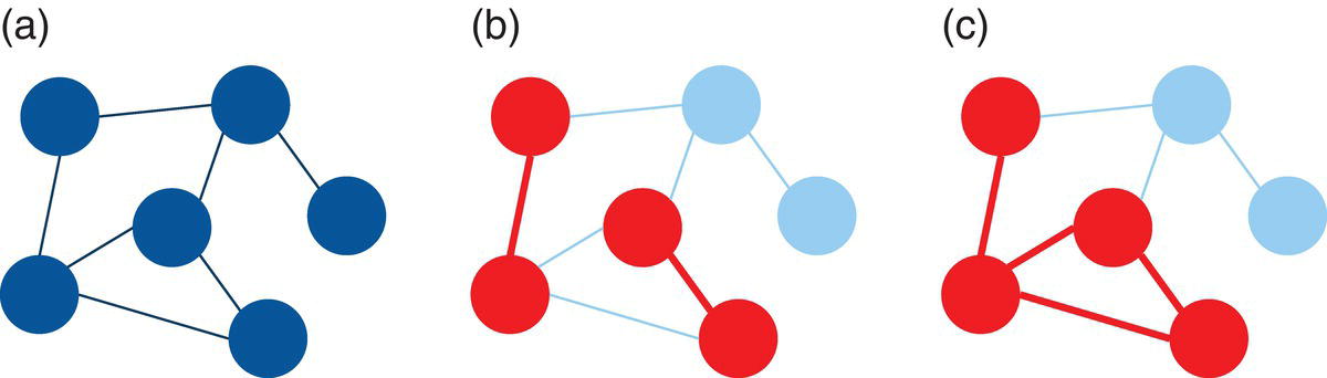
Figure 2.1 (a) Graph (b) Subgraph (c) Induced graph.
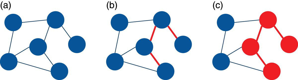
Figure 2.2 (a) Graph (b) Links selection (c) Subgraph by links selection.
Notice that the three links in (b) selected as part of the subgraph from the original graph in (a) also brings the fours nodes connected by them, creating the subgraph in (c).
When a subgraph is defined based on a subset of nodes, which is quite common, it is called a node induced subgraph of the original graph. When a subgraph is defined by selecting a subset of links, it is called a link induced subgraph of the original graph.
In addition to reducing the size of the original network, one of the most common reasons we use subgraphs when analyzing network is to understand the impact of removing nodes and links from the original graph; how the subnetwork would look if some actors or relationships are removed from the original network. This approach is quite important to better understand how significant a particular actor is, or how important specific relationships are. Eventually, by removing an actor, or a relationship, the original network is split into multiple subnetworks, disconnected from each other. That means that actor or relationship is absolutely crucial in the original network. Eventually, the network will keep a similar interconnectivity, still allowing the other actors to reach out to each other through other actors or other relationships. It means removing that actor or that relationship from the original network is not too important and doesn't much change the overall network connectivity.
For example, in a star graph, the central node plays a very important role holding the network together. If the central node is removed from the original network, all satellite nodes will be isolated from each other. This case is shown in Figure 2.3.
Notice that the central node in the star graph connects all other nodes in the graph. If this node is removed from the original network, all other nodes will be isolated.
A specific connection can be also very important in a network. The following example shows that, if the central connection highlighted in the graph (a) is removed from the original graph, it will split the graph into two disconnected subgraphs in (b). In that case, one single connection can completely change the shape and the properties of the original network. This can be seen in Figure 2.4.
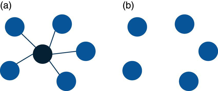
Figure 2.3 (a) Graph (b) Subgraph by removing nodes.
Removing nodes and links from the original network can therefore help us to understand the properties of the graph and the outcomes produced by these deletions. For example, how the final topology and structure of the subnetworks will look after removing particular nodes and links. Do these resulting subnetworks create communities, cores, cliques, or other different types of groups from the original network? What would be the importance of the removed nodes? What would be the relevance of the removed links? All these questions guide us to better exploring all the properties of the original network and identifying hidden patterns within the nodes and most important, within their relationships.
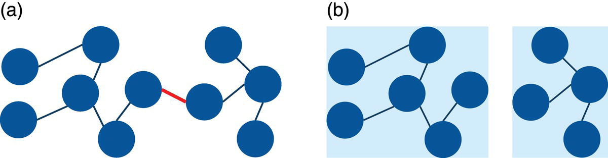
Figure 2.4 (a) Graph (b) Subgraphs by removing links.
2.1.1 Isomorphism
A frequent problem in network analysis and network optimization is known as the subgraph isomorphism problem. A subgraph isomorphism problem is a computational task that involves two graphs G and H as input. The problem is to determine if G contains a subgraph that is isomorphic to H. Two graphs are isomorphic to each other if they have the same number of nodes and links, and the link connectivity is the same. The following graphs and subgraphs exemplify the subgraph isomorphism problem. The subgraph G ′ of the graph G is isomorphic to the graph H. They have the same number of nodes and the same number of links. Also, the link connectivity is the same, which means the existing links connect the existing nodes within the graph and the subgraph in the same way. Figure 2.5 shows a case of isomorphism.
The subgraph isomorphism problem can be reduced to find a fixed graph as a subgraph in a given graph. The answer to the subgraph isomorphism question attracts many researchers and practitioners because many graph properties are hereditary for subgraphs. Ultimately, this means that a graph has a particular property if and only if all its subgraphs have the same property. However, the answer to this question can be computationally intensive. Finding maximal subgraphs of a certain type is usually a NP‐complete problem. The subgraph isomorphism problem is a generalization of the maximum clique problem or the problem of testing whether a graph contains a cycle, or a Hamiltonian cycle. Both problems are NP‐complete.
NP is a set of decision problems that can be solved by a non‐deterministic Turing Machine in polynomial time. NP is often a set of problems for which the correctness of each solution can be verified quickly, and a brute‐force search algorithm can find a solution by trying all workable solutions. Some heuristics are often used to reduce computational time here. The problem can be used to simulate every other problem for which a solution can be quickly verified whether it is correct or not. NP‐complete problems are the most difficult problems in the NP set. The problem, particularly in large networks, can be very computationally intensive. For instance, in the previous example, the very small graph G has another five other different subgraphs that are isomorphic to graph H. Graph G is a very small graph with just eight nodes and contains a total of six subgraphs isomorphic to graph H. In a very large network, the search for all possible subgraphs can be computationally exhaustive.
Analyzing subgraphs instead of the entire original graph becomes more and more interesting, especially in applications like social network analysis. Finding patterns in groups of people instead of in the entire network can help data scientists, data analysts, and marketing analysts to better understand customers' relationships and the impact of these relations in viral churn or influential product and service adoption. Particularly for large networks, we can find multiple distinct patterns throughout the original network when looking deeper into groups of actors. Each group might have a specific pattern, and it can be vastly different from the other groups. Understanding these differences may be a key factor not to just interpret the network properties but mostly to apply network analysis outcomes to drive business decisions and solve complex problems. The subgraph approach allows us to focus on specific groups of actors within the network, reducing the time to process the data and making the outcomes easier to interpret. The sequence of steps to divide the network into subnetworks, analyze less data, and more quickly interpret the outcomes can be automatically replicated to all groups within the network.
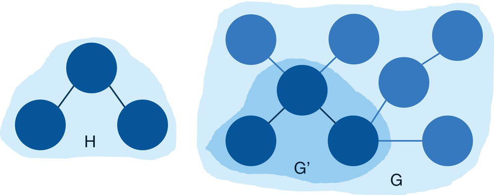
Figure 2.5 Subgraph G ′ isomorphic to graph H .
Many network problems rely on the concepts behind subgraphs. In this chapter we will focus on some of the most important subgraphs in network analysis and network optimization. This chapter covers, therefore, the concepts on connected components, biconnected components, and the role of the articulation points, communities, cores, reach networks (or ego networks), network projection, nodes similarity, and pattern match. Some other concepts on subgraphs like clique, cycle, minimum cut, and minimum spanning tree, for example, will be covered in the network optimization chapter.
2.2 Connected Components
A connected component is a set of nodes that are all reachable from each other. For a directed graph, there are two types of components. The first type is a strongly connected component that has a directed path between any two nodes within the graph. The second type is a weakly connected component, which ignores the direction of the graph and requires only that a path exist between any two nodes within the graph. Connected components describe that if two nodes are in the same component, then there is a path connecting these two nodes. The path connecting these two nodes may have multiple steps going through other nodes within the graph. All nodes in the connected component are somehow linked, no matter the number of nodes in between any pair.
Connected components can be calculated for both directed and undirected graphs. A graph can have multiple connected components. Therefore, a connected component is an induced graph where any two nodes are connected to each other by a path, but they are not connected to any other node outside the connected component within the graph.
Connected components are commonly referred to as just components of a graph. A common question in graph theory relies on the fact of whether or not a single node can be considered as a connected component. By definition, the answer would be yes. A graph can be formed by a single node with no link incident to it. A graph is connected if every pair of nodes in the graph can be connected by a path. Theoretically, a single node is connected to itself by the trivial path. Based on that, a single node in a graph would be also considered a component, or a connected component in that graph.
In proc network, the CONNECTEDCOMPONENTS statement invokes the algorithm that solves the connected component problem, or the algorithm that identifies all connected components within a given graph. The connected components can be identified for both directed and undirected graphs. Proc network uses three different types of algorithms to identify the connected components within a graph. The option ALGORITHM = has four options to either specify one of the three algorithms available or allow the procedure to automatically identify the best option. The option ALGORITHM = AUTOMATIC uses the union‐find or the afforest algorithms in case the network is defined as an undirected graph. If the network is defined as a directed graph, the option ALGORITHM = AUTOMATIC uses the depth‐first search algorithm to identify all connected components within the network. The option ALGORITHM = AFFOREST forces proc network to use the algorithm afforest to find all connected components within an undirected graph. Similarly, the option ALGORITHM = DFS forces proc network to use the algorithm depth‐first in order to find all connected components within a directed graph or an undirected graph. Finally, the option ALGORITHM = UNIONFIND forces proc network to use the union‐find algorithm to find all connected components within an undirected graph. The algorithm union‐find can also be executed in a distributed manner across multiple server nodes by using the proc network option DISTRIBUTED = TRUE. This option specifies whether or not proc network will use a distributed graph. By default, proc network doesn't use a distributed graph. The afforest algorithm usually scales well for exceptionally large graphs.
The final results for the connected component algorithm in proc network are reported in the output table defined by the options OUT =, OUTNODES =, and OUTLINKS=.
The option OUT = within the CONNECTEDCOMPONENTS statement produces an output containing all the connected components and the number of nodes in components.
- concomp: the connected component identifier.
- nodes: the number of nodes contained in the connected component.
The option OUTNODES = within the PROC NETWORK statement produces an output containing all the nodes and the connected component to which each one of them belongs.
- node: the node identifier.
- comcomp: the connected component identifier for the node.
The option OUTLINKS = within the PROC NETWORK statement produces an output containing all the links and the connected component each link belongs to.
- from: the origin node identifier.
- to: the destination node identifier.
- concomp: the connected component identifier for the link.
Let's see some examples of connected components in both directed and undirected graphs.
2.2.1 Finding the Connected Components
Let's consider a simple graph to demonstrate the connected components problem using proc network. Consider the graph presented in Figure 2.6. It shows a network with just 8 nodes and only 10 links. Weight links are not relevant when searching for connected components, just the existence of a possible path between any two nodes. As in many graph algorithms, when the input graph grows too large, the process can be increasingly exhaustive, and the output table can be extremely big.
The following code describes how to create the input dataset for the connected component problem. First, let's create only the links dataset, defining the connections between all nodes within the network. Later, we will see the impact of defining both links and nodes datasets to represent the input graph. The links dataset has only the nodes identification, the from and to variables specifying the origin and the destination nodes. When the network is specified as undirected, the origin and destination are not considered in the search. The direction doesn't matter here. Another way to think of the undirected graph is that every link is duplicated to have both directions. For example, a unique link A→B turns into two links A→B and B→A. This link definition doesn't provide a link weight as it is not considered when searching for the connected components.
data mycas.links;input from $ to $ @@;datalines;A B B C C A B D D H H E E F E G G F F D;run;
Once the input dataset is defined, we can invoke the connected component algorithm using proc network. The following code describes how this is done. Notice the links definition using the LINKSVAR statement. The variables from and to receive the origin and the destination nodes, respectively. As the name of the variables in the links definition are exactly the same names required by the LINKSVAR statement, the use of the LINKSVAR statement can be suppressed. We are going to keep the definition in the code (and in all of the codes throughout this book) as in most of the cases, the name of the nodes can be different than to and from, like caller and callee, origin and destination, departure and arrival, sender and receiver, among many others.
proc networkdirection = undirectedlinks = mycas.linksoutlinks = mycas.outlinksoutnodes = mycas.outnodes;linksvarfrom = fromto = to;connectedcomponentsout = mycas.concompout;run;
Figure 2.7 shows the outputs for the connected component algorithm. The first one reports a summary of the execution process. It provides a summary of the network, with 8 nodes and 10 links. Notice that we didn't provide a nodes dataset, even though proc network can derive the set of nodes from the links dataset. It also says the graph direction as undirected. The solution summary says that a solution was found, and only one connected component was identified. Finally, the output describes the three output tables created, the links output table, the nodes output table, and the connected components output table.
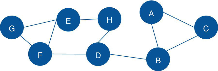
Figure 2.6 Input graph with undirected links.
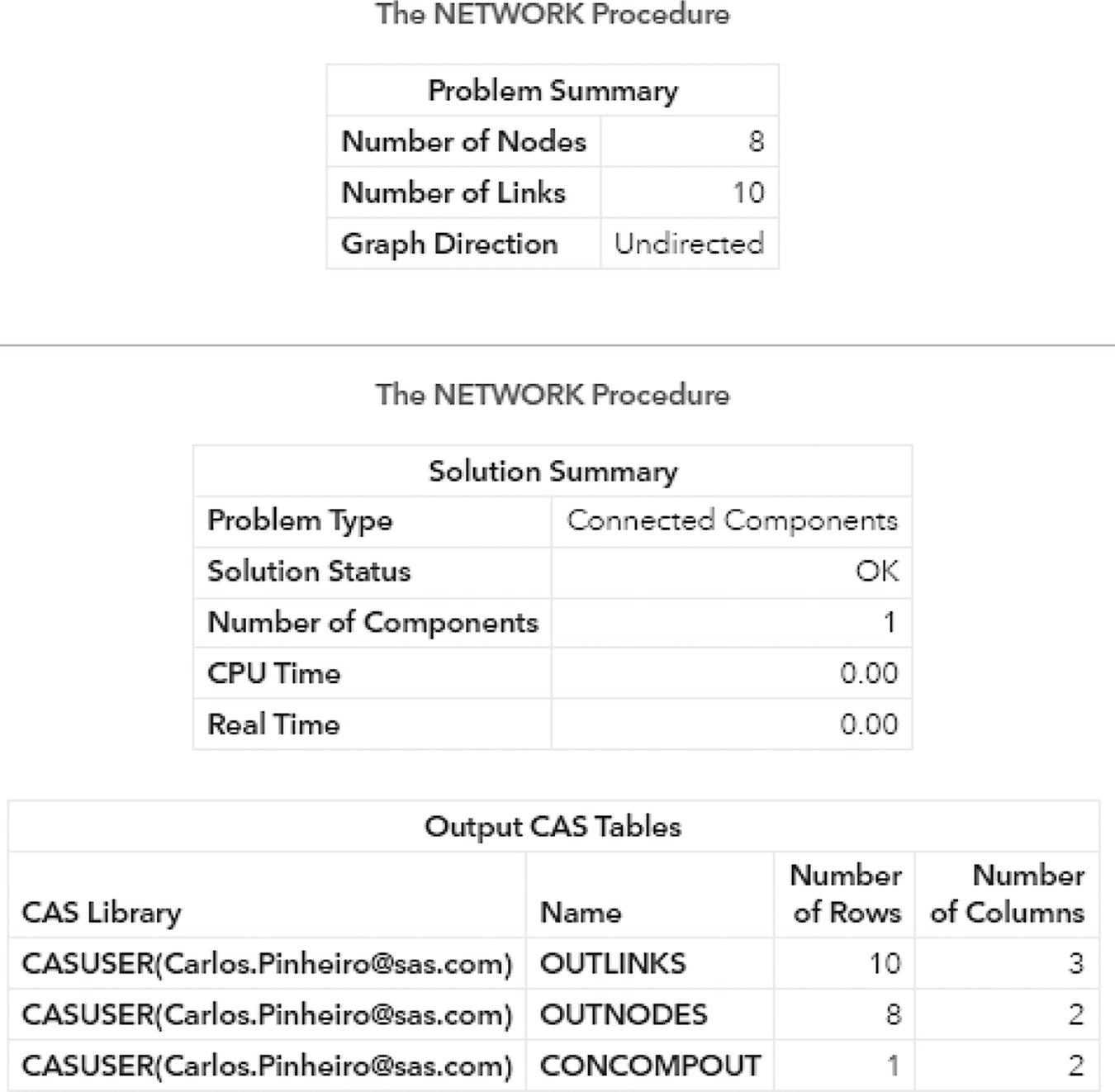
Figure 2.7 Output results by proc network running the connected components algorithm upon an undirected input graph.
The following figures show the connected components results. Figure 2.8 presents the OUTNODES table, which describes the nodes and the connected components which each node belongs to.
Notice that there is one single connected component. The undirected graph in this example allows for every node to be reached by any other within the network, based on some particular path.
Figure 2.9 shows the OUTLINKS table, which presents the links and the connected components they belong to. The output table describes the original links variables, from and to, and the connected component assigned to the link.
Finally, the output table CONCOMPOUT shows the summary of the connected component algorithm, presented in Figure 2.10. This table presents the connected components identifiers and the number of nodes in each component. As this undirected graph has one single connected component, this output table has one single row, showing the unique connected component 1 with all the eight nodes from the input graph.
As we can see, the original input graph, considering undirected links, presents one single connected component. What happens if we remove a few links from the original network? Let's recreate the links dataset without the three original links, H→E, D→H, and B→D. The following code shows how to recreate this new network based on that modified links dataset.
data mycas.links;input from $ to $ @@;datalines;A B B C C A E F E G G F F D;run;
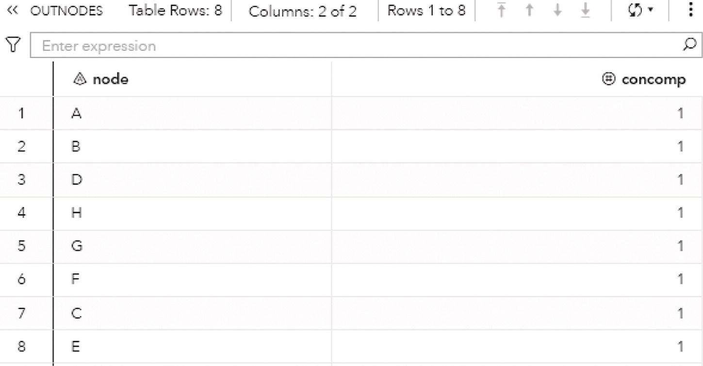
Figure 2.8 Output nodes table for the connected components.
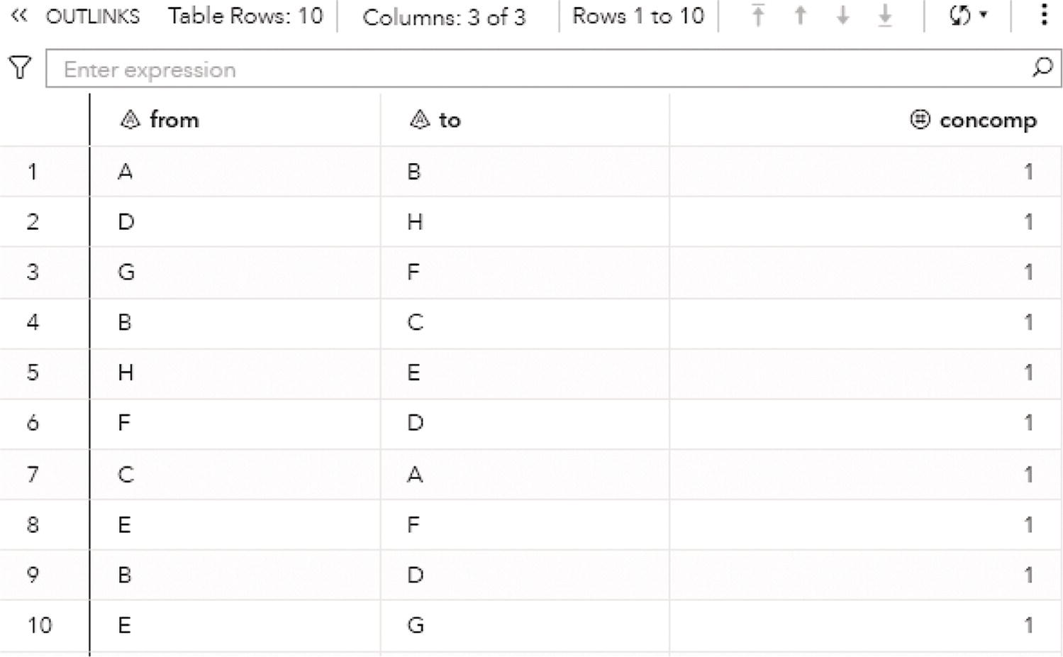
Figure 2.9 Output links table for the connected components.
In order to maintain the same set of nodes from the original network, we need to define a nodes dataset. Proc network assumes the set of nodes based on the provided set of links. As we remove the incident links to node H (H→E and D→H), node H wouldn't be in the links dataset and therefore, it wouldn't be in the presumed nodes dataset either. If we want to keep the same set of nodes, including node H from the original network, we need to provide the nodes dataset and force the presence of node H in the input graph. The following code creates the nodes dataset.
data mycas.nodes;input node $ @@;datalines;A B C D E F G H;run;
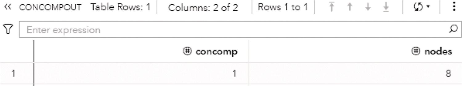
Figure 2.10 Output summary table for the connected components.
Once both links and nodes dataset s are created, we can rerun proc network and see how many connected components will be identified upon that new set of links and the declared set of nodes. The following code reruns proc network on the new links dataset and also considers the nodes dataset.
proc networkdirection = undirectedlinks = mycas.linksnodes = mycas.nodesoutlinks = mycas.outlinksoutnodes = mycas.outnodes;linksvarfrom = fromto = to;nodesvarnode = node;connectedcomponentsout = mycas.concompout;run;
Without the three original links H→E, D→H, and B→D, the new network will present three connected components. One of the components will contain a single node.
Figure 2.11 shows the new network without those three links and the declared set of nodes.
Proc network produces the output summary, stating that the input graph has eight nodes and now only seven links. A solution was found and three connected components were identified. The output tables OUTLINKS, OUTNODES, and CONCOMPOUT report all results. Figure 2.12 shows the summary results for the procedure.
The output table OUTLINKS shows all seven links associated with the input graph, and the connected component each link belongs to. Figure 2.13 shows the output table for the links.
The output table OUTNODES shows all the eight nodes associated with the input graph, and the connected component each one belongs to. Notice that the connected component 1 has three nodes (A, B, and C), the connected component 2 has four nodes (E, F, G, and D), and the connected component 3 has one single node (H). Figure 2.14 shows the output table for the nodes.
The output table CONCOMPOUT shows the connected components identified and the number of nodes of each component. The connected component 1 has three nodes, the connected component 2 has four nodes, and finally the connected component 3 has one single node. Figure 2.15 shows the output table for the connected components.
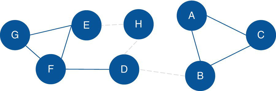
Figure 2.11 Input graph with undirected links.
Figure 2.16 shows the connected components highlighted within the original input graph.

Figure 2.12 Output results by proc network running connected components on undirected graph.
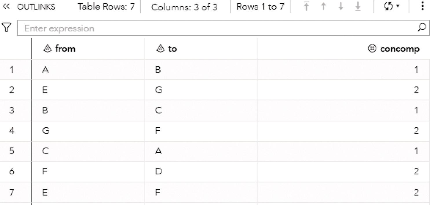
Figure 2.13 Output links table for the connected components.
Now, let's see how the connected components algorithm works upon a directed graph. In this example, we are going to use the exact same input graph defined at the beginning of this section, but the direction in proc network will be set as directed. The direction of each link will follow the links dataset definition.
The following code defines the set of links, and the from variable here actually specifies the origin or source node, and the to variable actually specifies the destination or sink node.
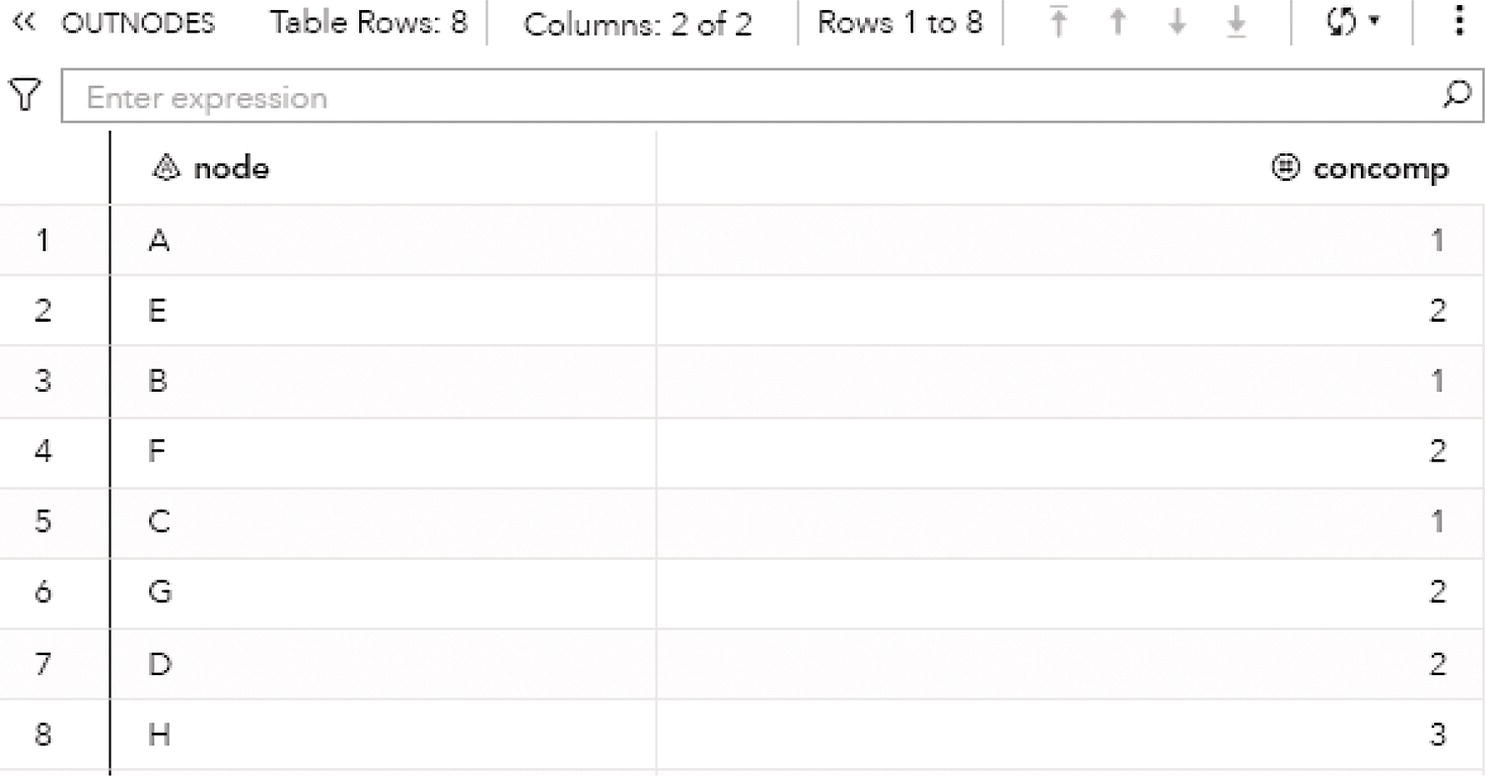
Figure 2.14 Output nodes table for the connected components.
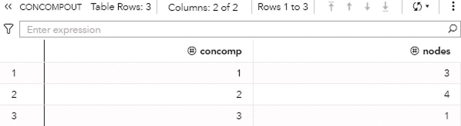
Figure 2.15 Output summary table for the connected components.
data mycas.links;input from $ to $ @@;datalines;A B B C C A B D D H H E E F E G G F F D;run;
The following code invokes proc network to identify the connected components within a directed graph. Notice the DIRECTION = DIRECTED statement in proc network.
proc networkdirection = directedlinks = mycas.linksoutlinks = mycas.outlinksoutnodes = mycas.outnodes;linksvarfrom = fromto = to;connectedcomponentsout = mycas.concompout;run;
Figure 2.17 shows the original input graph with the directed links. Note that the graph is exactly the same as the one presented previously, except for the direction of the links between the nodes.
The output summary produced by proc network shows the results of the connected components upon a directed graph. It has the same number of nodes and links, but now instead of one single component, two components are identified. Figure 2.18 shows the summary results for the connected components algorithm.
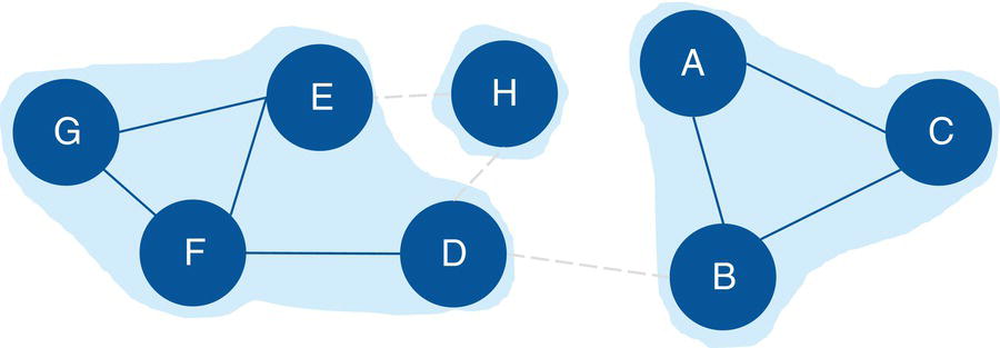
Figure 2.16 Input graph with undirected links and the identified connected components.
Figure 2.19 presents the output links for the connected components. The output table OUTLINKS shows all ten links associated with the input graph and the connected component each link belongs to. Notice that the link B→D does not belong to any connected component. This particular link is the one that breaks down the original directed input graph into two distinct components.
Figure 2.20 shows the output nodes for the connected components. The output table OUTNODES shows all the eight nodes associated with the input graph, and the connected component each one of them belongs to. Notice that the connected component 1 has three nodes (B, A, and C), and the connected component 2 has five nodes (D, E, G, H, and F).

Figure 2.17 Input graph with directed links.
Figure 2.21 shows the output connected components. The output table CONCOMPOUT shows the connected components identified and the number of nodes of each component. The connected component 1 has three nodes and the connected component 2 has five nodes.
Figure 2.22 shows the connected components highlighted within the original directed input graph.
When we analyze graphs, sometimes the focus is too much on the role of the nodes. In the next section, we clearly see this while we discuss the concept of biconnected components. However, the last example here also shows the importance of analyzing the roles of the links. The link B→D plays a fundamental role in splitting the original input graph into two disjoined components. In many practical cases and business scenarios, when analyzing graphs created by social or corporate interactions, we focus on the roles of the nodes. Nevertheless, it is important to keep in mind the significant role of the links. Sometimes, the links will reveal more useful insights about the social or corporate networks than the nodes themselves. Sometimes it is not about the entities in the network, but how these entities relate to each other.
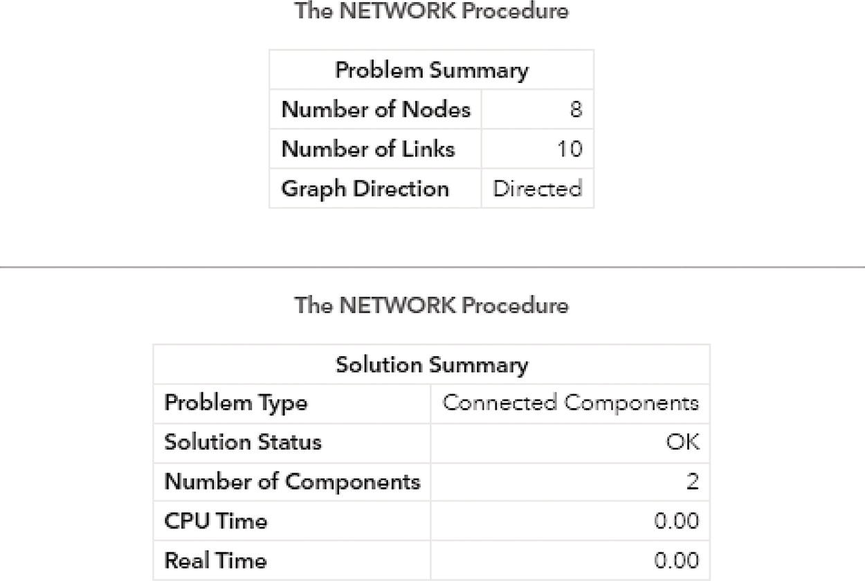
Figure 2.18 Output results by proc network running connected components on a directed graph.
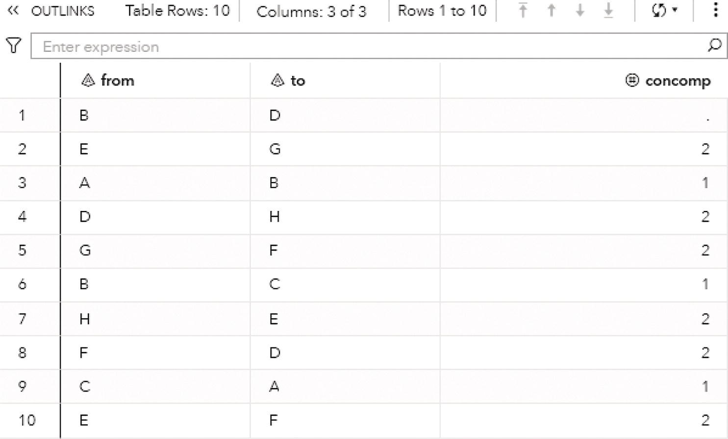
Figure 2.19 Output links table for the connected components.
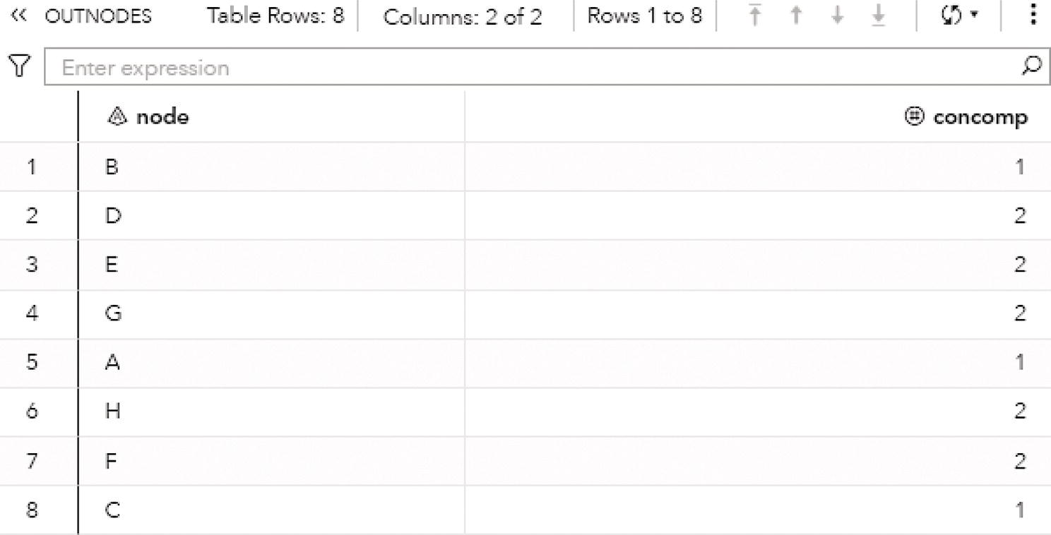
Figure 2.20 Output nodes table for the connected components.

Figure 2.21 Output summary table for the connected components.
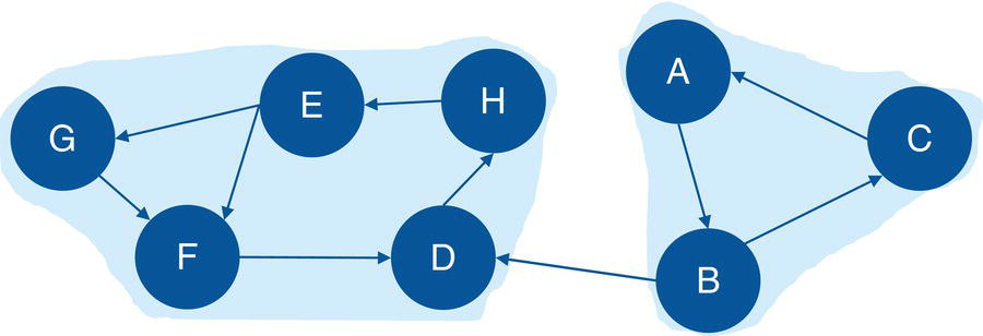
Figure 2.22 Input graph with directed links and the identified connected components.
2.3 Biconnected Components
A biconnected component of a graph G = (N, L) is a subgraph that cannot be broken into disconnected pieces by deleting any single node and its incidents links. If a component can be broken into other connected components, there is a node that if removed from the graph, will increase the number of connected components. This type of node is commonly called an articulation point.
Biconnected components can be seen as a variation of the connected components concept, meaning the graph may have some important nodes that can break down a component into smaller components. Sometimes the articulation points are also referred to as bridges, as these nodes create bridges between different groups or components within the network.
Articulation points often play an important role when analyzing graphs that represent any sort of communications network. For example, suppose a graph G = (N, L) and an articulation point i ∈ N. If the articulation point i is removed from the graph G, it will break down the graph into two components C 1 and C 2. All paths in G between nodes in C 1 and nodes C 2 must pass through node i. The articulation point i is crucial to keep the communication flow within the original component or graph.
Depending on the context, particularly in scenarios associated with communication networks, the articulation points can be viewed as points of vulnerability in a network. Roads and rails represented by graphs, supply chain processes, social and political networks, among other types, are graphs where the articulation points represent vulnerabilities within the network, either breaking down the components into more connected components, or stopping the communication flow within the network. Imagine a bridge connection two locations. These two locations can represent articulation points and can stop the network flow not just between these two locations, but among the locations that are adjacent to them. Terrorist networks are also a fitting example of the importance of the articulation points. Commonly, targeting and eliminating individuals that represent articulation points within the network can strategically break down the power of a cohesive component into smaller and disorganized groups.
In proc network, the BICONNECTEDCOMPONENTS statement invokes the algorithm that solves the biconnected component problem, or the algorithm that identifies all biconnected components within a given graph. Different from the connected components, which can be identified in both directed and undirected graphs, the biconnected components can be identified only for the undirected graphs. In order to compute and identify the biconnected components, proc network uses a variant of the depth‐first search algorithm. This algorithm can scale large graphs.
The final results for the biconnected component algorithm in proc network are reported in the output table defined by the options OUT =, OUTNODES =, and OUTLINKS =. The option OUT = within the BICONNECTEDCOMPONENTS statement produces an output containing all the biconnected components and the number of links associated with each of them.
- biconcomp: the biconnected component identifier.
- links: the number of links contained in the biconnected component.
The biconnected components are more associated with the links within the graph than to the nodes. Therefore, the option OUTNODES = within the PROC NETWORK statement produces an output containing all the nodes identification, and a flag to determine whether or not each node is an articulation point.
- node: the node identifier.
- artpoint: identify whether or not the node is an articulation point. The value of 1 determines that the node is an articulation point. The value of 0 determines that the node is not an articulation point.
The option OUTLINKS = within the PROC NETWORK statement produces an output containing all the links and the biconnected component each link belongs to.
- from: the origin node identifier.
- to: the destination node identifier.
- biconcomp: the biconnected component identifier for the link.
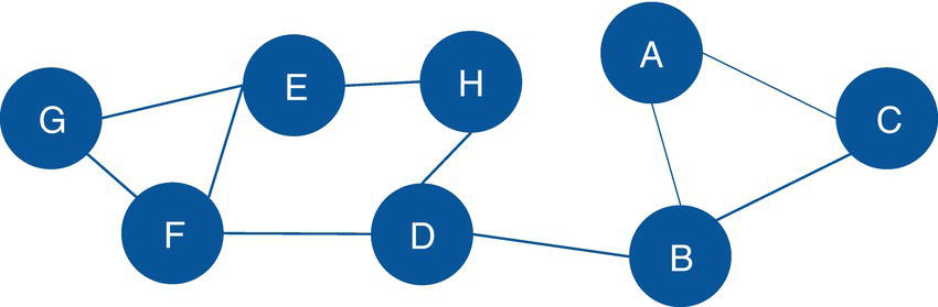
Figure 2.23 Input graph with undirected links for the biconnected components identification.
Let's see an example of connected components for an undirected graph.
2.3.1 Finding the Biconnected Components
Let's consider the same graph we have used for the connected components example. That graph is shown in Figure 2.23 and has 8 nodes and 10 links. Similar to the connected components, links weights are not required when searching for biconnected components.
The following code describes the links dataset creation. No weights are required, just the origin and destination nodes for the undirected graph.
data mycas.links;input from $ to $ @@;datalines;A B B C C A B D D H H E E F E G G F F D;run;
Based on the links dataset, we can invoke the biconnected component algorithm to reach for the biconnected components and the articulation point nodes within the graph. The following code describes how to do that.
proc networkdirection = undirectedlinks = mycas.linksoutlinks = mycas.outlinksoutnodes = mycas.outnodes;linksvarfrom = fromto = to;biconnectedcomponentsout = mycas.biconcompout;run;
The following picture shows the outputs for the biconnected components algorithm. Figure 2.24 reports a summary of the execution process, showing the network composed of 8 nodes and 10 links, as an undirected graph. A solution was found with three biconnected components being identified and with two nodes being determined as articulation points. The last part of the output describes the three output tables created, the links output table, the nodes output table, and the biconnected components output table.
Figure 2.25 shows the OUTLINKS table, which describes the links and the biconnected components each link belongs to. The output table describes the original links variables from and to, and the biconnected component identifier assigned to the link.
Notice that there are three biconnected components. The biconnected component 1 comprises three links, C→A, A→B, and B→C. The biconnected component 2 comprises one single link, B→D. Finally, the biconnected component 3 comprises six links, E→F, D→H, G→F, H→E, F→D, and E→G.
Figure 2.26 shows the OUTNODES table, which describes the nodes and the articulation point flag.
Two nodes were identified as articulation points, which means they can break down the connected component into smaller components within the input graph. The nodes B and D can represent bridges in the original network splitting the original graph into multiple subgraphs.
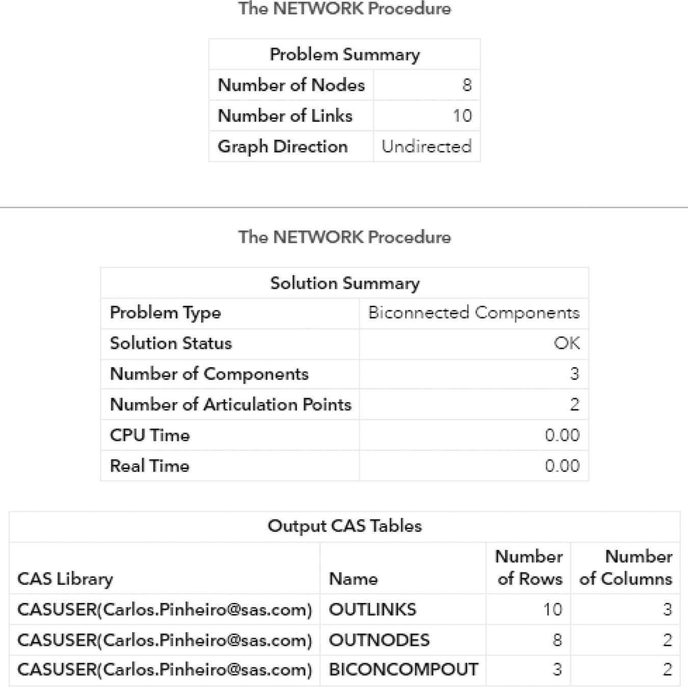
Figure 2.24 Output results by proc network for the biconnected components algorithm.
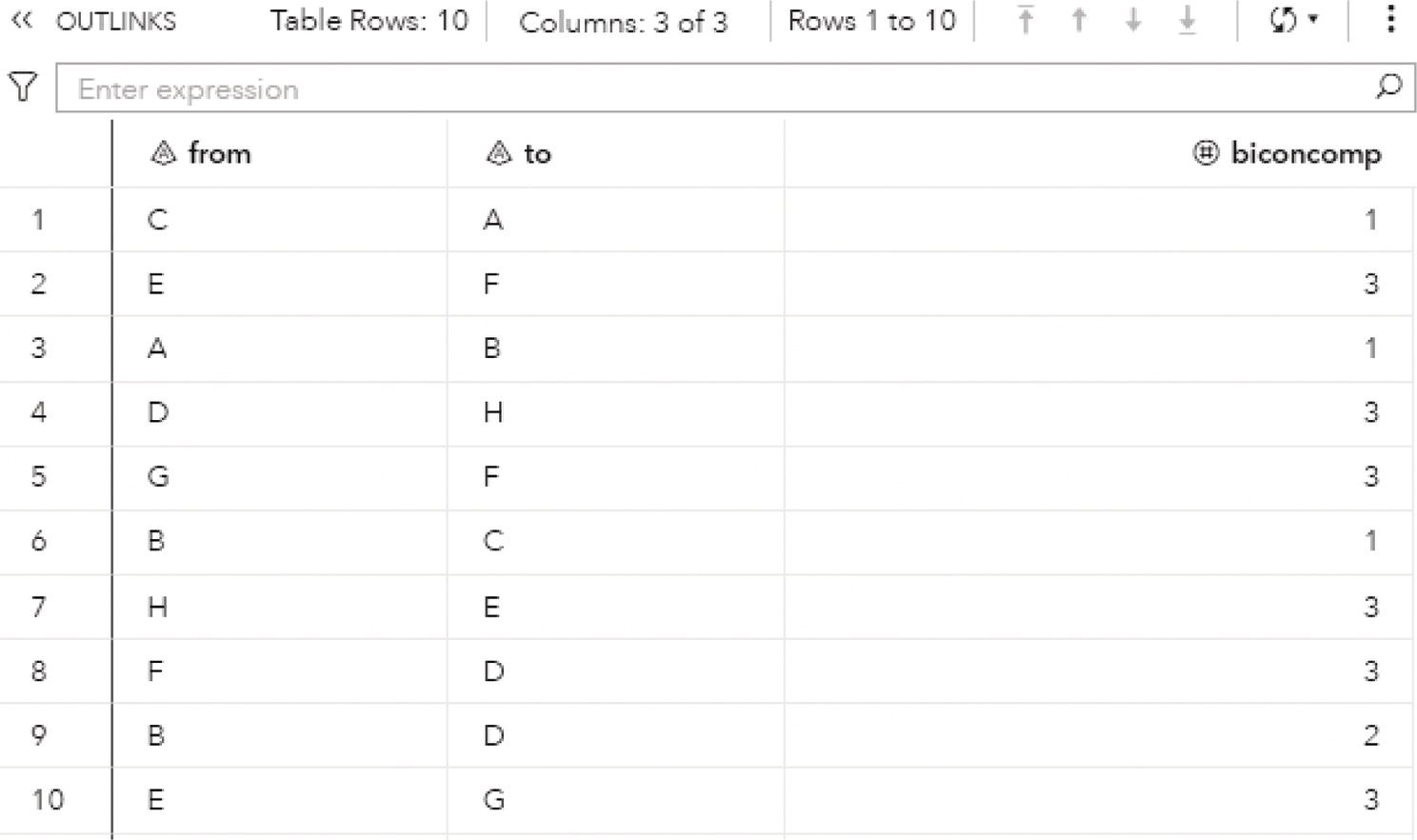
Figure 2.25 Output links table for the biconnected components.
Finally, the output table BICONCOMPOUT shows the summary of the biconnected component algorithm. It is presented in Figure 2.27. This table presents the biconnected components identifiers and the number of links in each biconnected component. As described above, biconnected component 3 has six links, biconnected component 2 has one single link, and biconnected component 1 has three links.
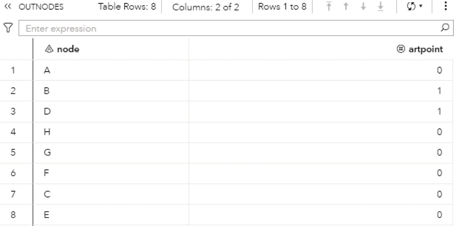
Figure 2.26 Output nodes table for the biconnected components.
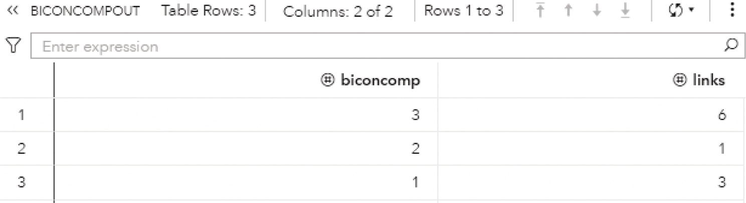
Figure 2.27 Output summary table for the biconnected components.
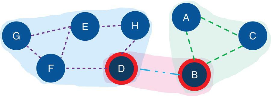
Figure 2.28 Input graph with the identified biconnected components and the articulation point nodes.
Figure 2.28 shows the biconnected components highlighted within the original input graph, as well as the articulation point nodes.
Notice on the left that six links create one biconnected component. On the right, three links create another biconnected component. In the middle of the graph, a single link creates the last biconnected component. On the left biconnected component, if we remove node E, nodes G and F still can reach out to node H through node D. If we remove node H, node D still can reach out to node E through node F. Therefore, nodes G, F, E, H, and D form a unique biconnected component. By removing any of these nodes, we still cannot break apart the original component into two or more smaller components. The same thing happens for nodes A, B, and C. Removing any of these nodes does not break apart the original component into smaller components. The remaining nodes will still be able to connect to each other. Only nodes D and B have the ability to break apart the original component into smaller components. If we remove node D, the nodes G, F, E, and H will form a component, and node A, B, and C will for another one. If we remove node B, nodes A and C will form a component, and nodes G, F, E, H, and D will form another one. For this reason, nodes D and B are the articulation points within this input graph.
2.4 Community
Community detection is a crucial step in network analysis. It breaks down the entire network into smaller groups of nodes. These groups of nodes are more connected among them than between that group and the others. The idea of community detection is to join nodes based on their average link weights. The average link weights inside the communities should be greater than the average link weight between the communities. Nodes are gathered based on the strength of their relationships in comparison to the rest of their connections.
Communities are densely connected subgraphs within the network where nodes belonging to the same community are more likely to be connected to nodes within their own communities than to nodes outside their communities. A network can contain as many communities as the number of nodes, or one single community representing the entire network. Often, something in between that captures the overall characteristics of different groups of nodes while keeping the network topology structure. Similar to clustering analysis, the community detection algorithm assigned to each node to a unique community.
The idea of communities within networks is very intuitive and quite useful when analyzing large graphs. As groups of nodes densely connected, the concept of communities is commonly found in networks representing social interactions, chemistry and biological structures, and grids of computers, among other fields. Community detection is important to identify customers consuming the same service, products being purchased together (like in association rules or market basket analysis), companies most frequently making transactions together, or just groups of people who are densely related to each other. Notice that community detection is not clustering analysis. Both techniques combine observations into groups. Clustering works on the similarity of the observations' attributes. For example, customers' demographics or consuming habits. Customers with no relation can fit into the same group just based on their similar attributes. Community detection combines observations (nodes) based on their relations, or the strength of their connections to each other. In fact, this is the fundamental difference between common machine learning or statistical models and network analysis. The first always looks into observations attributes, and the second always looks into observations connections.
There are two primary methods to detect communities within networks, the agglomerative methods, and the divisive methods. Agglomerative methods add links one by one to subgraphs containing only nodes. The links are added from the higher link weight to the lower link weight. Divisive methods perform a completely opposite approach. In divisive methods, links are removed one by one from the subgraphs. Both methods can find multiple communities upon the same network, with different numbers of members in them. It is hard to say which method is the best, as well as what is the best number of communities within a network and the average number of members in them. Mathematically, we can use metrics of resolution and modularity to narrow this search, but in most cases, a domain knowledge is important to understand what makes sense for each particular network. For example, let's say that in a telecommunications network, the average number of relevant distinct connections for each subscriber is around 30. When detecting communities within this network, we should try to find a particular number of communities that represent a similar number of mem'ers in each community on average. Suppose that carrier has around 120 million subscribers. Finding 2 or 3 million communities wouldn't be absurd. That number would give us around 40‐60 as an average number of members in each community. Community detection is important in understanding and evaluating the structure of large networks, like the ones associated with communications, social media, banking, and insurance, among others.
The community detection algorithm was initially created to be used on undirected graphs. Currently, there are some algorithms that provide alternative methods to compute community detection on directed graphs. If we are working on directed graphs and still want to perform a community detection using algorithms for undirected graphs, we need to aggregate the links between the pair of nodes, considering both directions, and sum up their weights. Once the links are aggregated and the links weighted are summed up, we can invoke a community detection algorithm designed to detect communities on undirected graphs. Figure 2.29 describes that scenario.
The method of partitioning the network into communities is an iterative process, as described before. Two types of algorithms to partition a graph into subgraphs can be used upon undirected links. Proc network implements both heuristics methods, called Label Propagation and Louvain. Proc network also implements a particular algorithm to partition a graph into communities based on directed links, called Parallel Label Propagation. All three methods for finding communities in directed and undirected graphs are heuristic algorithms, which means they search for an optimal solution, speeding up the searching process by employing practical methods that reach satisfactory solutions. The solution found doesn't mean that the solution is perfect.
The Louvain algorithm aims to optimize modularity, which is one of the most popular merit functions for community detection. Modularity is a measure of the quality of a division of a graph into communities. The modularity of a division is defined to be the fraction of the links that fall within the communities, minus the expected fraction if the links were distributed at random, assuming that the degree of each node does not change.

Figure 2.29 Aggregating directed links into undirected links.
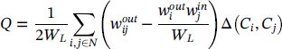
The modularity can be expressed by the following equation:
where Q is the modularity, W ij is the sum of all link weights in the graph G = (N, L), w ij is the sum of the link weights between nodes i and j, C i is the community to which node i belongs, C j is the community to which node j belongs, and ∆(C i , C j ) is the Kronecker delta defined as:
The following is a brief description of the Louvain algorithm:
- Initialize each node as its own community.
- Move each node from its current community to the neighboring community that increases modularity the most. Repeat this step until modularity cannot be improved.
- Group the nodes in each community into a super node. Construct a new graph based on super nodes. Repeat these steps until modularity cannot be further improved or the maximum number of iterations has been reached.
The label propagation algorithm moves a node to a community to which most of its neighbors belong. Extensive testing has empirically demonstrated that in most cases, the label propagation algorithm performs as well as the Louvain method.
The following is a brief description of the label propagation algorithm:
- Initialize each node as its own community.
- Move each node from its current community to the neighboring community that has the maximum number of nodes. Break ties randomly, if necessary. Repeat this step until there are no more movements.
- Group the nodes in each community into a super node. Construct a new graph based on super nodes. Repeat these steps until there are no more movements or the maximum number of iterations has been reached.
The parallel label propagation algorithm is an extension of the basic label propagation algorithm. During each iteration, rather than updating node labels sequentially, nodes update their labels simultaneously by using the node label information from the previous iteration. In this approach, node labels can be updated in parallel. However, simultaneous updating of this nature often leads to oscillating labels because of the bipartite subgraph structure often present in large graphs. To address this issue, at each iteration the parallel algorithm skips the labeling step at some randomly chosen nodes in order to break the bipartite structure.
For directed graphs, the modularity equation changes slightly.
where ![]() is the sum of the weights of the links departing from node i and arriving at node j,
is the sum of the weights of the links departing from node i and arriving at node j, ![]() is the sum of the weights of the links outgoing from node i, and
is the sum of the weights of the links outgoing from node i, and ![]() is the sum of the weights of the links incoming to node j.
is the sum of the weights of the links incoming to node j.
All three algorithms adopt a heuristic local optimization approach. The final result often depends on the sequence of nodes that are presented in the links input data set. Therefore, if the sequence of nodes in the links data set changes, the result can be different.
The graph direction is relevant in the community detection process. For undirected graphs, both algorithms; Louvain and label propagation; find communities based on the density of the subgraphs. For directed graphs, the algorithm parallel label propagation finds communities based on the information flow along the directed links. It propagates the community identification along the outgoing links of each node. Then, when using directed graphs, if the graph does not have a circle structure where nodes are connected to each other along outgoing links, the nodes are likely to switch between communities during the computation. As a result, the algorithm might not converge well and then a good community structure within the graph might not be established.
We always need to think about the graph direction depending on the problem we are analyzing. For example, in a social network, the definition of friendship is represented by undirected links. For a telecommunications or banking network, the call, text, or money transfer are represented by directed links. However, the community detection approach can still be performed by both directed and undirected graphs. For instance, in the telecommunications network, even though the relationships between subscribers are represented by directed links, it makes sense to detect communities based on an undirected graph, as both directions for calls and texts ultimately create the overall relation among people. Perhaps for the banking network, detect communities based on directed links makes more sense as the groups of accounts would be based on the information flow, or the sequence of transactions.
A crucial step in community detection is always to analyze the outcomes and verify if the groups found make sense in the context of the business or the problem to be solved. For example, If the parallel label propagation algorithm does not converge for the directed graphs and poor communities are detected, a reasonable approach is to perform the community detection based on undirected graphs. If the label propagation does not work well in finding proper communities upon undirected graphs, we can always try the Louvain algorithm, and vice versa. Changing parameters for the recursive option, or the resolution used are also options to better detect reasonable communities. The community detection is ultimately a trial and error process. We need to spend time executing multiple runs and analyzing the outcomes until we decide the best structure and partitioning.
Another point of attention is the size of the network. For large networks, a power law distribution is commonly observed in terms of the average number of nodes within the communities, which results in few communities with a large number of members, and most of the communities with a small number of nodes. There are some approaches to reduce this effect, by using some of the parameters mentioned before, like the resolution list and the recursive methods. A combination of approaches can also be deployed, usually providing reliable results. For example, we can first perform community detection based on the resolution list, and then adjust the partitioning by using the recursive method considering solely the best resolution in the last step.
In proc network, the COMMUNITY statement invokes the algorithm to detect communities within an input graph. There are many options when running community detection in proc network. The first and probably the most important one is the decision about which algorithm to use. The option ALGORITHM = specifies the algorithm to be used during the community detection process, one of the three algorithms previously mentioned. ALGORITHM = LOUVAIN specifies that the community detection will be based on the algorithm Louvain. It runs only for undirected graphs. ALGORITHM = LABELPROP specifies that the community detection will be performed based on the label propagation algorithm. It can be used only for undirected graphs. Finally, the option ALGORITHM = PARALLELLABELPROP specifies that the community detection will be based on the parallel label propagation algorithm. Although this algorithm is designed to directed graphs, it can also run based on undirected graphs.
The FIX = option specifies which variable in the nodes input table will define the group of nodes that need to be together in a community. This option is only used for undirected graphs, which means it is available when the ALGORITHM = option is LOUVAIN or LABELPROP. The idea behind this option is to allow users to define a group of nodes to be together, in the same community, no matter the result of the community detection based on the partitioning algorithm. Usually, community detection algorithms start by assigning each node as one community and then progressively changing nodes between communities based on the type of the algorithm and the set of parameters defined. The variable specified in the FIX = option should be in the nodes input table defined in the NODES = option. This variable must contain a nonnegative integer value. Nodes with the same value are forced to be in the same community. Regardless of the partitioning process, they cannot be split into different groups along the community detection process. These nodes that are forced into the same community still can be merged or split into larger or smaller communities, but they must be together in the same community. For example, a nodes dataset NodeSetIn has a variable called comm to determine the nodes that must be together. The option NODES = NodeSetIn defines the nodes input table. The option FIX = comm specifies the variable to be used during the partitioning process. Let's say nodes A, B, and C have comm equal to 1, and nodes X, Y, and Z have comm equal to 2. All other nodes have missing values for comm. During the community detection process, proc network will force that nodes A, B, and C fall into the same community, and nodes X, Y, and Z fall into the same community as well. They can be in the same community (all of them together), or in two distinct communities (A/B/C together in one and X/Y/Z together in another), but they cannot be split into multiple communities. The community detection algorithm basically treats the group of nodes that are required to be in the same community as a single unit, like a “supernode”. A straightforward consequence of fixing nodes to be in the same community by using the FIX = option is that proc network will have fewer options to move these nodes around into different communities. The overall number of node movements will be drastically reduced according to the number of nodes set to be together. The other consequence is that less communities with more members may be found.
The WARMSTART = option works similarly to the FIX = option, at least at the beginning of the process. This option specifies which variable in the nodes input table will define the group of nodes that need to be together when the partitioning process starts. This option defines the initial partition for warm starting community detection. This initialization can be based on prior executions of community detection, or according to existing knowledge about the data, the problem or the business scenario involved. Similar to the FIX = option, the nodes that have the same value in the variable defined in the option WARMSTART are placed in the same community. All other nodes with missing values in that variable or not specified in the nodes input table, are placed in their own community. The warm start just places the nodes together at the beginning of the partitioning process. During the community detection execution, those nodes can move around to different communities and can end up falling into distinct groups. For example, a nodes dataset NodeSetIn has a variable called startcomm to determine the nodes that must be placed together when the graph partitioning process starts. The option NODES = NodeSetIn defines the nodes input table. The option FIX = startcomm specifies the variable to be used during the community detection process. Let's say nodes A, B, and C have startcomm equal to 1, and nodes X, Y, and Z have startcomm equal to 2. All other nodes have missing values for startcomm. At the beginning of the partitioning, nodes A, B, and C will form a single community. Nodes X, Y, and Z will form another community. All other nodes will be their own community. Nodes A, B, and C, as well as X, Y, and Z, will be treated as a “supernode” ABC and XYZ, respectively. They can change communities along the partitioning, but they need to be placed together at the beginning.
Notice that both FIX = and WARMSTART = options can be used at the same time. When both options are specified simultaneously, the values of the variables defined for fix and warm start are assumed to be related. For example, if nodes A and B have a value of 1 for the fix, and node C has a value of 1 for the warm start, then they are initialized in the same community. However, during the partitioning, the algorithm can move node C to a different community than nodes A and B, but nodes A and B are forced to move together to another community. At the end of the process, A and B are forced to be in the same community, while C can end up in a different one.
The RECURSIVE option recursively breaks down large communities into smaller groups until some certain conditions are satisfied. The RECURSIVE option provides a combination of three possible sub options, MAXCOMMSIZE, MAXDIAMETER, and RELATION. These options can be used individually or simultaneously. For example, we can define RECURSIVE (MAXCOMMSIZE = 100) to define a tentative maximum of 100 members for community, or RECURSIVE (MAXCOMMSIZE = 500 MAXDIAMETER = 3 RELATION = AND) to define the maximum number of members for each community as 500 and the maximum distance between any pair of nodes in the community as 3. Both conditions must be satisfied during the graph partitioning as the sub option RELATION is defined as AND. The sub option MAXCOMMSIZE defines the maximum number of nodes for each community. The sub option MAXDIAMETER defines the maximum number of links within the shortest paths between any pair of nodes within the community. The diameter represents the largest number of links to be traversed in order to travel from one node to another. It is the longest shortest path of a graph. The sub option RELATION defines the relationship between the other two sub options, MAXCOMMSIZE and MAXDIAMETER. If RELATION = AND, the recursive partitioning continues until both constrains defined in MAXCOMMSIZE and MAXDIAMETER sub options are satisfied. If RELATION = OR, the partitioning continues until either the maximum number of members in any community is satisfied or the maximum diameter is reached.
At the first step, the community detection algorithm processes the network data with no recursive option. At the end of each step, the algorithm checks if the community outcomes satisfy the criteria defined in the recursive option. If the criteria are satisfied, the recursive partitioning stops. If the criteria are not satisfied yet, the recursive partition continues on each large community (the ones do not satisfy the criteria) as an independent subgraph and the recursive partitioning is applied to each one of them. The criteria define the maximum number of members for each community and the maximum distance between any pair of nodes within each community. However, the recursive method only attempts to limit the size of the community and the maximum diameter. The criteria are not guaranteed to be satisfied as in certain cases; some communities can no longer be split. Because of that, at the end of the process, some communities can have more members than defined in MAXCOMMSIZE or more links between a pair of nodes than defined in MAXDIAMETER.
The RESOLUTIONLIST option specifies a list of values that are used as a resolution measure during the recursive partitioning. The list of resolutions is interpreted differently depending on the algorithm used for the community detection. The algorithm Louvain uses all values defined in the resolution list and computes multiple levels of recursive partitioning. At the end of the process, the algorithm produces different numbers of communities, with different numbers of members in them. For example, higher resolution tends to produce more communities with less members, and low resolution tends to produce less communities with more members. This algorithm detects communities at the highest level first, and then merges communities at lower levels, repeating the process until the lowest level is reached. All levels of resolution are computed simultaneously, in one single execution. This allows the process to be computed extremely fast, even for large graphs. On the other hand, the recursive option cannot be used. If the recursive option is used in conjunction with the resolution list, only the default resolution value of 1 is used and the list of multiple resolutions is ignored. Also, because of the nature of this optimization algorithm, two different executions most likely will produce two different results. For example, a first execution with a resolution list of 1.5, 1.0, and 0.5, and a second execution with a resolution list of 2.0 and 0.5 can produce different outcomes at the same resolution level of 0.5. This happens mostly because of the recursive merges happening throughout the process from higher resolutions to lower ones.
The algorithm parallel label propagation executes the recursive partitioning multiple times, one for each resolution specified. Because of that, the resolution list in the parallel label propagation algorithm is fully compatible with the recursive option. Every execution of the community detection algorithm will use one resolution value and the recursive criteria. In the parallel label propagation, the resolution value is used when the algorithm decides to which neighboring communities a node should be fit. A node cannot fit to a community if the density of the community, after adding the node, is less than the resolution value r. The density of a community is defined as the number of existing links in the community divided by the total number of possible links, considering the current set of nodes within it. As this algorithm runs in parallel when deciding about which community to fit a node, the final communities are not guaranteed to have their densities larger than the resolution value at all times. The parallel label propagation algorithm may not converge properly if the resolution value specified is too large. The algorithm will probably create many small communities, and the nodes will tend to change between communities along the iterations. On the other hand, if the resolution value is too small, the algorithm will probably find a small number of communities large. The use of the recursive option could be an approach to break down those large communities into smaller ones. Notice that, the larger the network, the longer it will take to properly run this process.
The algorithm label propagation is not compatible with the resolution list option. If a resolution list is specified when the label propagation algorithm is defined, the default resolution value of 1 is used instead.
The resolution can be interpreted as a measure to merge communities. Two communities are merged if the sum of the weights of intercommunity links is at least r times the expected value of the same sum if the graph is reconfigured randomly. Large resolutions produce more communities with a smaller number of nodes. On the contrary, small resolutions produce fewer communities with a greater number of nodes. Particularly for the algorithm Louvain, the resolution list enables running multiple community detections simultaneously. At the end of the recursive partitioning process multiple communities can be found at the same execution. This approach is interesting when searching for the best topology, particularly in large networks. However, this approach requires further analysis on the outcomes in order to identify the best community distribution. There are two main approaches to analyze the community distribution. The first one is by looking at the modularity value for each resolution level. Mathematically, the higher the modularity, the better. The resolution that gives the modularity closest to 1 provides the best topology in terms of community distribution. The second approach relies on the domain knowledge and the context of the problem. The number of communities and the average number of members in each community can be driven based on previous executions or upon a business understanding of the problem. The best approach is commonly a combination of the mathematical and business methods looking for a good modularity but restricting the number of communities and the average number of members in each community based on the domain knowledge.
The LINKREMOVALRATIO = option specifies the percentage of links with small weights will be removed from each node neighborhood. This option can dramatically reduce the execution time when running community detection on large networks by removing unimportant links between nodes. A link is removed if its weight is relatively smaller than the weights of the neighboring links. For example, suppose there are links A→B, A→C, and A→D with link weights 100, 80, and 1, respectively. When nodes are merged into communities, links A→B and A→C are more important than link A→D, as they contribute more to the overall modularity value. Because of that, link A→D can be removed from the network. By removing link A→D, node A will be connected only to nodes B and C. Node D will be disconnected to A when the algorithm merge nodes into communities. It doesn't mean that node D is removed from the network. Perhaps node D has strong links to other nodes in the graph and will be connected to them in a different community. If the weight of any link is less than the number specified in the LINKREMOVALRATIO = option divided by 100 and multiplied by the maximum link weight among all links incident to the node, that link will be removed from the network. The default value for the link removal ratio is 10.
The MAXITERS = option specifies the maximum number of iterations the community detection algorithm runs during the recursive partitioning process. For the Louvain algorithm, the default number of times is 20. For the parallel label propagation and the label propagations algorithms, the default number of times is 100.
The RANDOMFACTOR = option specifies the random factor for the parallel label propagation algorithm in order to avoid nodes oscillating in parallel between communities. At each iteration of the recursive partitioning, the number specified in the option is the percentage of the nodes that are randomly skipped to the step. The number varies from 0 to 1. For example, 0.1 means that 10% of the nodes are not considered during each iteration of the algorithm.
The RANDOMSEED = option works together with the random factor in the parallel label propagation algorithm. The random factor defines the percentage of the nodes that will be not considered at each iteration of the partitioning. In order to consider a different set of random nodes at each iteration, a number must be specified to create the seed. The default seed is 1234.
The TOLERANCE = option or the MODULARITY = option specifies the tolerance value to stop the iterations when the algorithm searches for the optimal partitioning. The Louvain algorithm stops iterating when the fraction of modularity gain between two consecutive iterations is less than the number specified in the option. The label propagation and parallel label propagation stop iterating when the fraction of community changes for all nodes in the graph is less than the number specified in the option. The value for this option varies from 0 to 1. The default value for the Louvain and the label propagation algorithms is 0.001, and for the parallel label propagation algorithm is 0.05.
The community detection process can produce up to six outputs as a result. These datasets describe the network structure in terms of the communities found based on the set of nodes, the set of links, the different levels of executions when the community detection uses the algorithm Louvain with multiple resolutions, the properties of the communities, the intensity of the nodes within the communities, and how the communities are connected. To produce all these outcomes, the community detection algorithm may consume considerable time and storage, particularly for large networks. In that case, we may consider suppressing some of these outcomes that are mostly intended for post community detection analysis.
The option OUTNODES = within the COMMUNITY statement produces an output containing all nodes and their respective community. In the case of multiple resolutions, the output reports the community for each node at each resolution level. After the topology is selected, all nodes are uniquely identified to a community, at each resolution level. Post analysis of the communities can be performed based on the nodes and their communities upon each level executed.
- node: identifies the node.
- community_i: identifies the community the node belongs to, where i identifies the resolution level defined in the resolution list, and i is ordered from the greatest resolution to the lowest in the list.
The option OUTLINKS = contains all links and their respective communities. Again, if multiple resolutions are specified during the community detection process, the output reports the community for each link at each resolution level. If the link contains the from node assigned to one community and the to node assigned to a different community, the community identifier receives a missing value to describe that link belongs to inter‐communities.
- from: identifies the originating node.
- to: identifies the destination node.
- community_i: identifies the community the link belongs to, where i identifies the resolution level defined in the resolution list and is ordered from the greatest to the lowest resolution in the list.
The option OUTLEVEL = contains the number of communities and the modularity values associated with the different resolution levels. This outcome is probably one of the first outputs to be analyzed in order to identify the possible network topology in terms of communities. The balance between the modularity value, the number of communities found, and the average number of members for all communities is evaluated at this point.
- level: identifies the resolution level.
- resolution: identifies the value in the resolution list.
- communities: identifies the number of communities detected on that resolution list.
- modularity: identifies the modularity achieved for the resolution level when the community detection process is executed.
The option OUTCOMMUNITY = contains several attributes to describe the communities found during the community detection process.
- level: identifies the resolution level.
- resolution: identifies the value in resolution list.
- community: identifies the community.
- nodes: identifies the number of nodes in the community.
- intra_links: identifies the number of links that connect two nodes in the community.
- inter_links: identifies the number of links that connect two nodes within different communities. For example, from node in one community and to node in a different community than from node.
- density: the intra_links divided by the total number of possible links within the community.
- cut_ratio: the inter_links divided by the total number of possible links from the community to nodes outside the community.
- conductance: the fraction of links from a node in the community that connects to nodes in a different community. For undirected graphs, it is the inter_links divided by the sum of inter_links, plus two times the intra_links. For directed graph, it is the inter_links divided by the sum of inter_links, plus intra_links.
These measures are especially useful in analyzing the communities, particularly in large graphs. The density and the intra links show how dense and well connected the community is, no matter its size or the number of members. The inter links, the cut ratio, and the conductance describe how isolated the community is from the rest of the network, or how interconnected it is to other communities within the network. Communities more interconnected to the rest of the network tend to spread the information flow faster and stronger. This characteristic can be used to diffuse marketing and sales information. Spare or highly isolated communities can be unexpected and can indicate possible suspicious behaviors. All these analyzes certainly depend on the context of the problem.
The option OUTOVERLAP = contains information about the intensity of each node. Even though a node belongs to a single community, it may have multiple links to other communities. The intensity of the node is calculated as the sum of the link weights it has with nodes within its community, divided by the sum of all link weights it has (considering link to nodes to the same community and to nodes within different communities). For directed graphs, only the outgoing links are taken into consideration. This output can be expensive to compute and store, particularly in large networks. For that reason, this output contains only the results achieved by the smallest value of the resolution list. This output table is one of the first options to be suppressed when working on large networks.
- node: identifies the node.
- community: identifies the community.
- intensity: identifies the intensity of the node that belongs to the community.
Finally, the option OUTCOMMLINKS contains information about how the communities are interconnected. This information is important to understand how cohesive the network is in a community's perspective.
- level: identifies the resolution level.
- resolution: identifies the value in the resolution_list.
- from_community: identifies the community of the from community.
- to_community: identifies the community of the to community.
- link_weight: identifies the sum of the link weights of all links between from and to communities.
Let's look into some different examples of community detection for both directed and undirected networks.
2.4.1 Finding Communities
Let's consider the following graph presented in Figure 2.30 to demonstrate the community detection algorithm. This graph has 13 nodes and 15 links. Link weights in community detection is crucial and defines the recursive partitioning of the network into subgraphs. The links in this network are first considered undirected. Multiple algorithms will be used and therefore, different communities will be detected.

Figure 2.30 Input graph with undirected weighted links.
The following code creates the input dataset for the community detection algorithm. The links dataset contains origin and destination nodes plus the weight of the links. Both algorithms Louvain and label propagation are used. Later, the same network is be used as a directed graph to demonstrate the parallel label propagation algorithm.
data mycas.links;Input from $ to $ weight @@;datalines;A B 10 B C 15 B J 12A F 2 A E 3 A D 2 C D 1 F E 2G F 12 G I 20 G H 11 K F 8D L 18 D E 10 M E 14;run;
As the input dataset is defined, we can now invoke the community detection algorithm using proc network. The following code describes how to define the algorithm and other parameters when searching for communities. In the LINKSVAR statement the variables from and to receive the origin and the destination nodes, even though the direction is not used at this first run. The variable weight receives the weight of the link. In the COMMUNITY statement, the ALGORITHM option defines the Louvain algorithm. The RESOLUTIONLIST option defines three resolutions to be used during the recursive partitioning. Notice that all three resolutions will be used in parallel, identifying distinct communities' topologies at a single run. Resolutions 2.5, 1.0, and −0.15 are defined for this search.
proc networkdirection = undirectedlinks = mycas.linksoutlinks = mycas.outlinksoutnodes = mycas.outnodes;linksvarfrom = fromto = to;communityalgorithm=louvainresolutionlist = 2.5 1.0 0.15outlevel = mycas.outcommleveloutcommunity = mycas.outcommoutoverlap = mycas.outoverlapoutcommLinks = mycas.outcommlinks;run;
The following pictures show the several outputs for the community detection algorithm. Figure 2.31 reports the summary for the execution process. It provides the size of the network, with 13 nodes and 15 links, and the direction of the graph. The solution summary states that a solution was found and provides the name of all output tables generated during the process.
Particularly for the Louvain algorithm, when multiple resolutions are used, the first output table analyzed is the OUTCOMMLEVEL. This output shows the result of each resolution used, the number of communities found, and the modularity achieved. It is presented in Figure 2.32.
As described before, the higher the modularity closest to one, the better the distribution of the nodes throughout the communities identified. The highest modularity for this execution is 0.5915, assigned to the level 2, using resolution 1.0, where 3 communities were found.
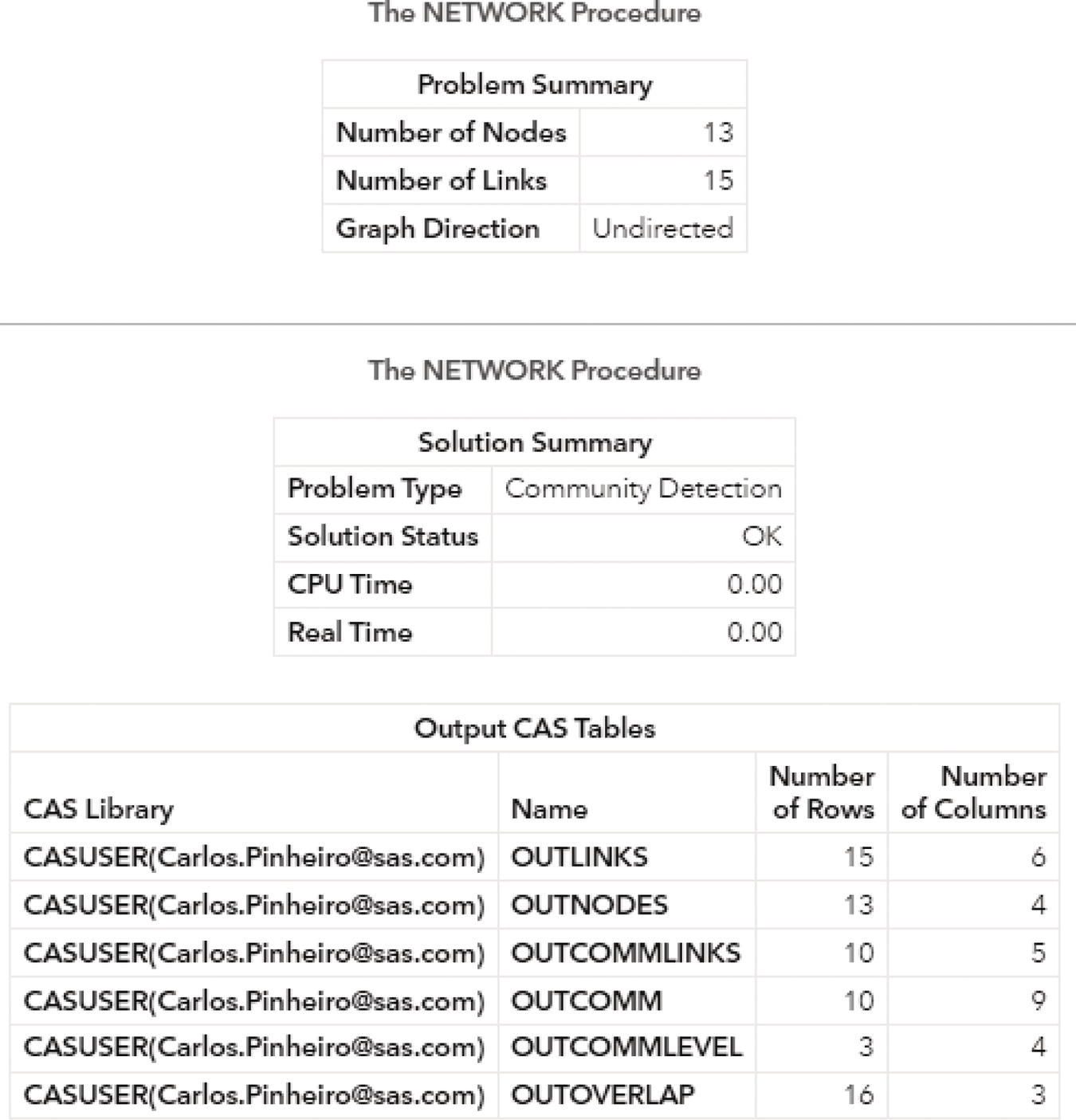
Figure 2.31 Output summary results for the community detection on an undirected graph.
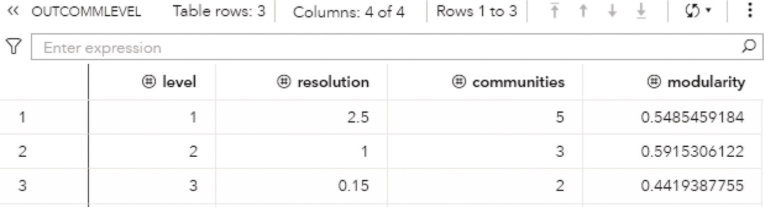
Figure 2.32 Output communities level table for the community detection.
The OUTNODES table presented in Figure 2.33 shows the nodes and the communities they belong to for each resolution used. For example, for the best resolution (level 2), the variable community_2 specifies which node is assigned to each community.
For the level 2, nodes A, B, C, and J fall into community 1, nodes D, E, L, and M fall into community 2 and nodes F, G, H, I, and K fall into community 3.
The OUTLINKS table presented in Figure 2.34 shows all links and the community they belong to for each resolution used. Notice that some links do not belong to any community and do not have a community identifier assigned. These links connect nodes that fall into different communities. For example, nodes A and D are connected in the original network but belong to different communities, 1 and 2. Then, these particular links do not belong to any community and receive a missing value.
The OVERLAP table presented in Figure 2.35 shows the nodes, which community or communities they belong to, and their intensity on each community. For example, node A belongs to community 1 with intensity 0.88 and to community 2 with intensity 0.11. Remember that the intensity of a node measures the ratio of the sum of the link weights with nodes within the same community by the sum of the link weights with all nodes. The intensity of node A in community 1 is much higher than the intensity in community 2, and in this case, it makes more sense that node A belongs to community 1.
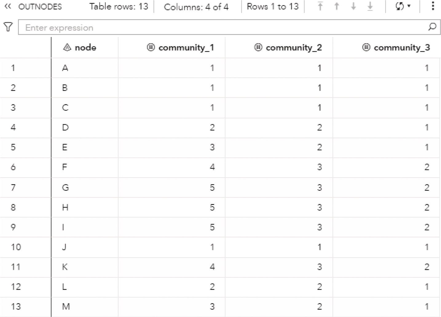
Figure 2.33 Output nodes table for the community detection.
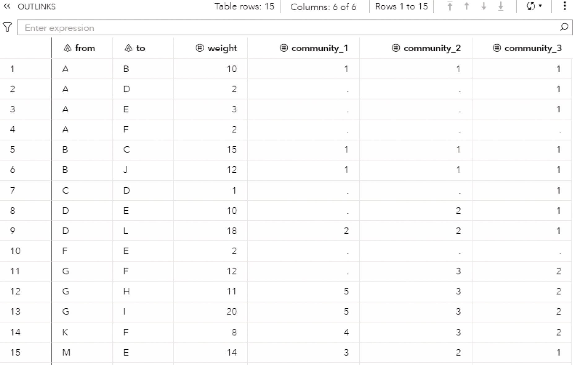
Figure 2.34 Output links table for the community detection.
The OUTCOMM table presented in Figure 2.36 shows the communities' attributes, for each level, or the resolution specified, the community identifier, the number of nodes, the intra links, the inter links, the density, the cut ration, and the conductance:
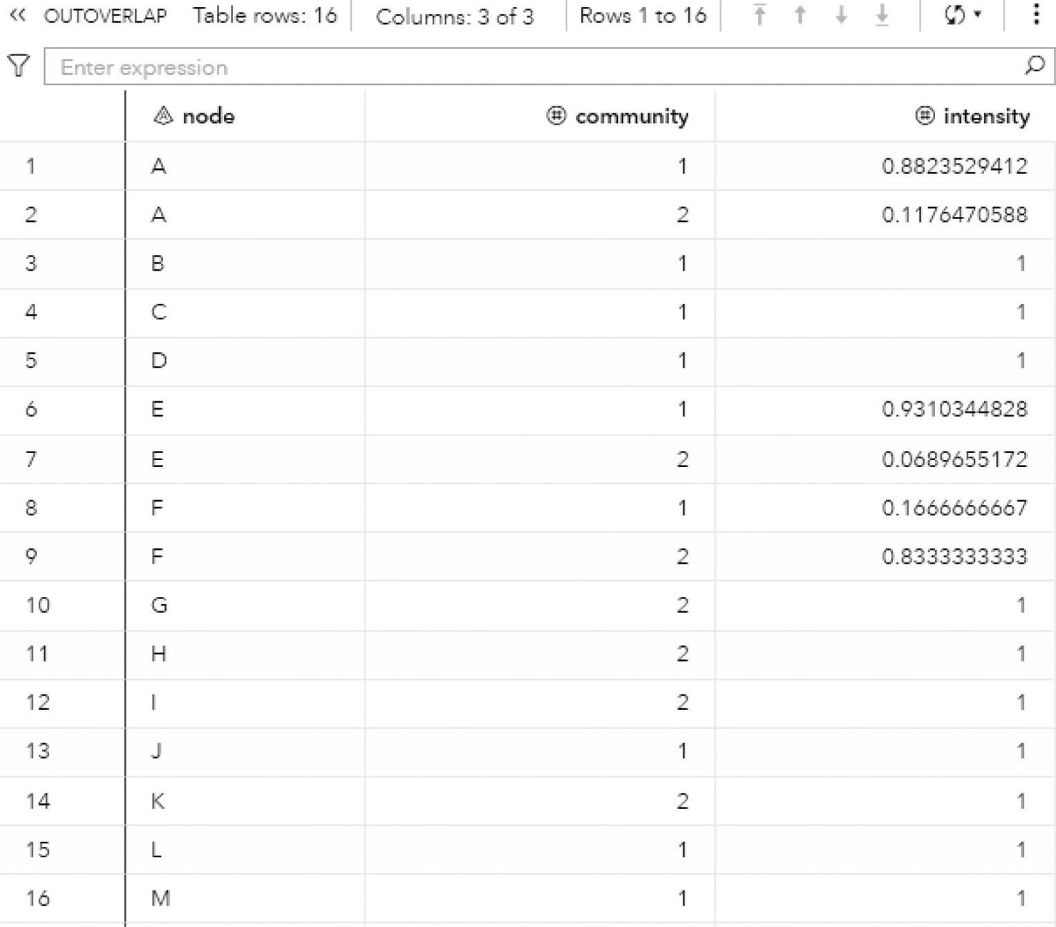
Figure 2.35 Output overlap table for the community detection.
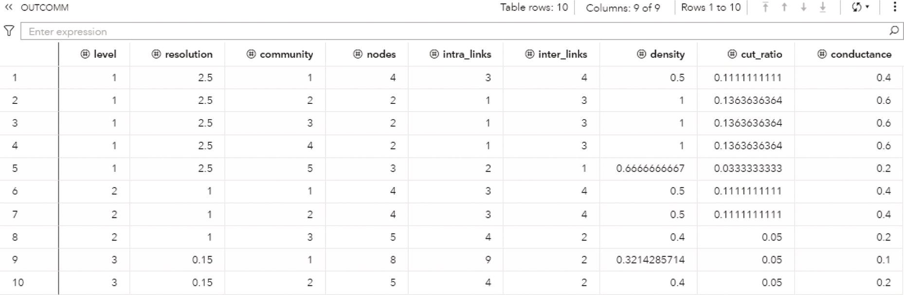
Figure 2.36 Output communities' attributes table for the community detection.
The OUTCOMMLINKS table presented in Figure 2.37 shows how the communities are connected, providing the links between the communities and the sum of the link weights.
Figure 2.38 shows the best topology for the community detection, highlighting the three communities identified and their nodes.
The Louvain algorithm found three different community topologies based on three distinct resolutions. The best resolution, the one which achieved the highest modularity, and identified three communities. Let's see how the other algorithms work and what happens when other options like the recursive approach are used.
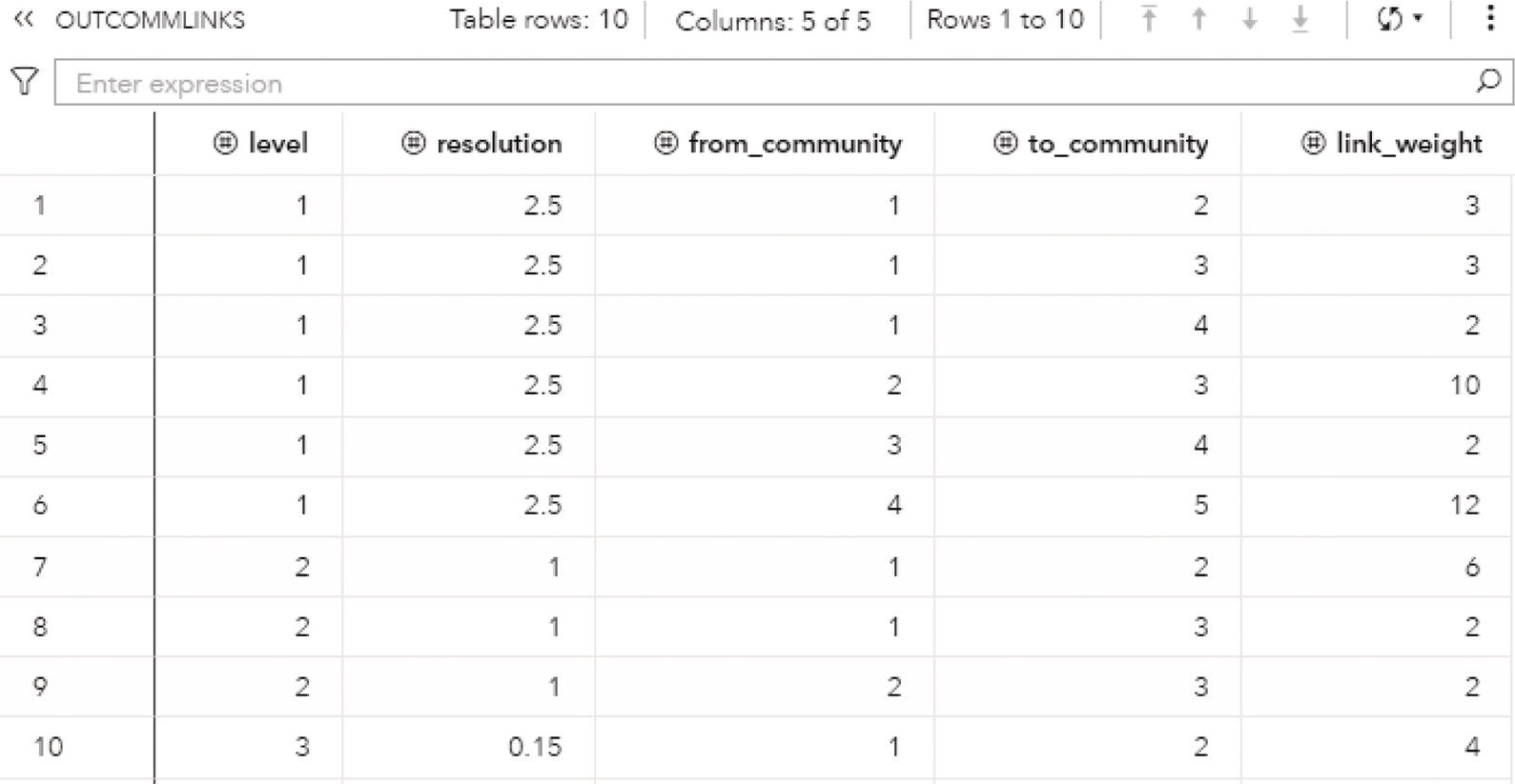
Figure 2.37 Output communities' links table for the community detection.

Figure 2.38 Communities identified by the Louvain algorithm.
The following code describes how to invoke the label propagation algorithm. A list of resolutions can be defined, but only the first one is used. If the resolution list is not specified, the default value of 1 is used. Any other value can be used but the resolution list must be specified with the value wanted.
proc networkdirection = undirectedlinks = mycas.linksoutlinks = mycas.outlinksoutnodes = mycas.outnodes;linksvarfrom = fromto = to;communityalgorithm=labelpropresolutionlist = 1.0outlevel = mycas.outcommleveloutcommunity = mycas.outcommoutoverlap = mycas.outoverlapoutcommLinks = mycas.outcommlinks;run;
The OUTCOMMLEVEL table presented in Figure 2.39 shows the final result for the community detection based on the label propagation algorithm. Resolution 1.0 represents level 1, where 4 communities were found. The modularity achieved was 0.5738, lower than the 0.5915 achieved by the Louvain algorithm based on the same resolution.
The OUTNODES table presented in Figure 2.40 shows the distribution of the nodes throughout the communities found. Now, nodes A, B, C, and J form the community 1, nodes D and L form the community 2, nodes F, G, H, I, and K form community 3, and finally nodes E and M form community 4. Notice that in the previous community detection, based on the Louvain algorithm, nodes D, L, E, and M formed one single community, and now they are split into two distinct communities.
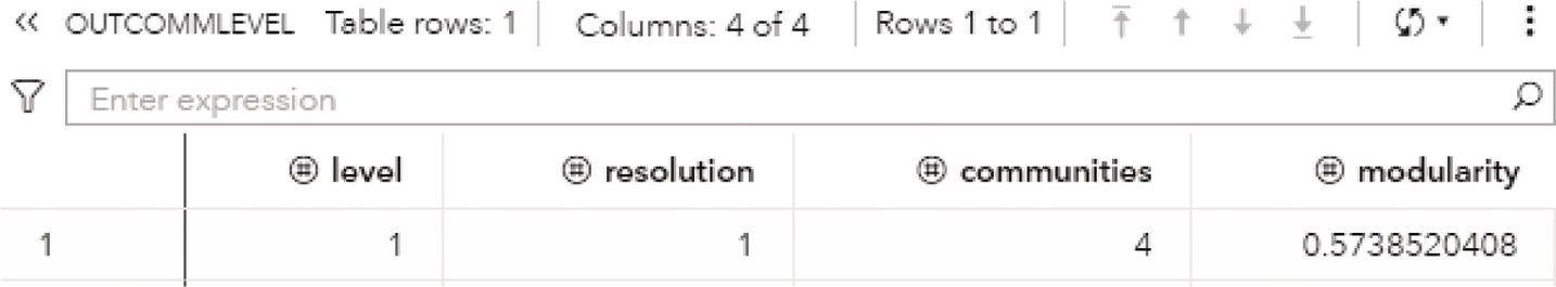
Figure 2.39 Output communities' level table for the community detection.
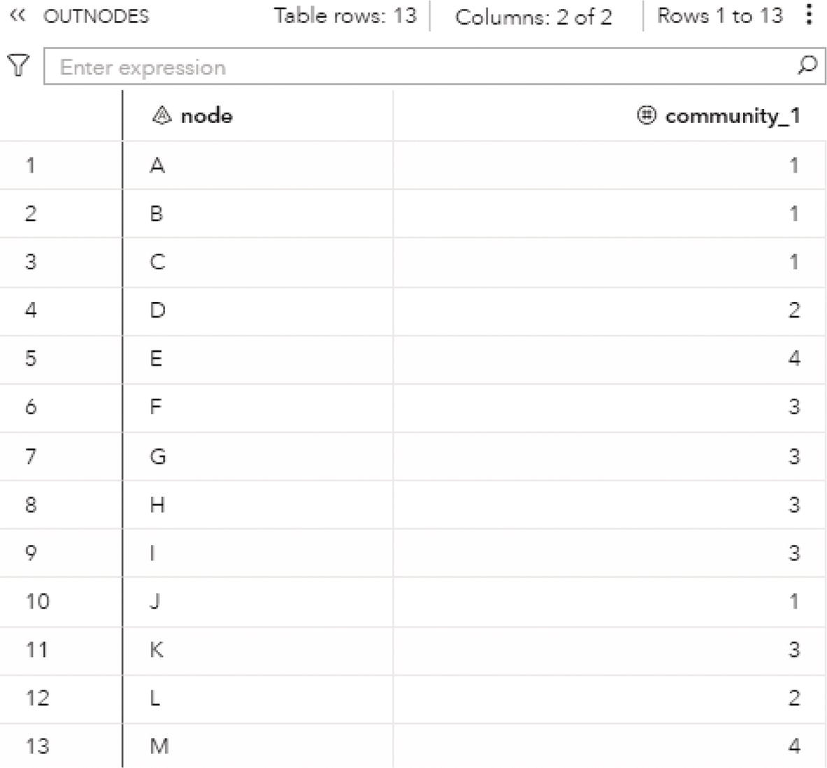
Figure 2.40 Output nodes table for the community detection.
Figure 2.41 shows the final community topology for the label propagation algorithm, highlighting the 4 communities detected.
Now, let's use the recursive option and see the results for the community detection. The algorithm used is still the label propagation. The recursive option specifies a maximum of 4 members for each community and the maximal diameter of 3 (the distance between any pair of nodes within the same community).
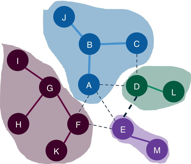
Figure 2.41 Communities identified by the label propagation algorithm.
Proc networkdirection = undirectedlinks = mycas.linksoutlinks = mycas.outlinksoutnodes = mycas.outnodes;linksvarfrom = fromto = to;communityalgorithm=labelpropresolutionlist = 1.0recursive(maxcommsize=4 maxdiameter=3 relation=and)outlevel = mycas.outcommleveloutcommunity = mycas.outcommoutoverlap = mycas.outoverlap;run;
The OUTCOMMLEVEL table presented in Figure 2.42 shows the final result for this particular community detection. Based on the label propagation algorithm and the recursive option, 5 communities were found.
The OUTNODES table presented in Figure 2.43 shows the distribution of the nodes throughout the communities. Nodes A, B, C, and J form the community 1, nodes D and L form the community 2, nodes E and M form community 3, nodes G, H, and I form community 4, and nodes F and K form community 5. Finally, notice that in the previous community detection, based on the Louvain algorithm, nodes D, L, E, and M formed one single community, and now they are split into two distinct communities. Also, notice that the previous community 3 was split into two distinct communities, 4 and 5.
Figure 2.44 shows the final community topology for the label propagation algorithm with the recursive option, highlighting the 5 communities detected.
The parallel label propagation algorithm is designed specifically for directed graphs. In order to demonstrate the process, let's use the same input graph, presented in Figure 2.45, but now considering the order of the links definition in the dataset as the direction of the connection.
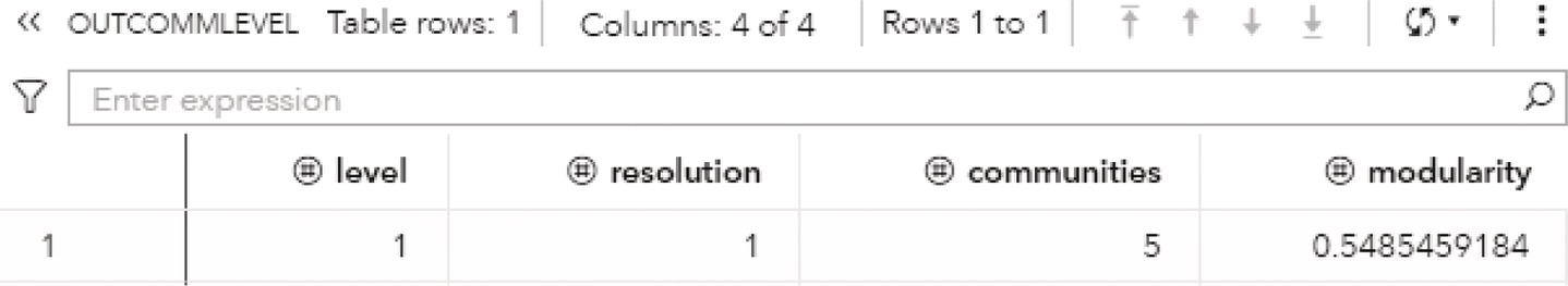
Figure 2.42 Output communities' level table for the community detection.
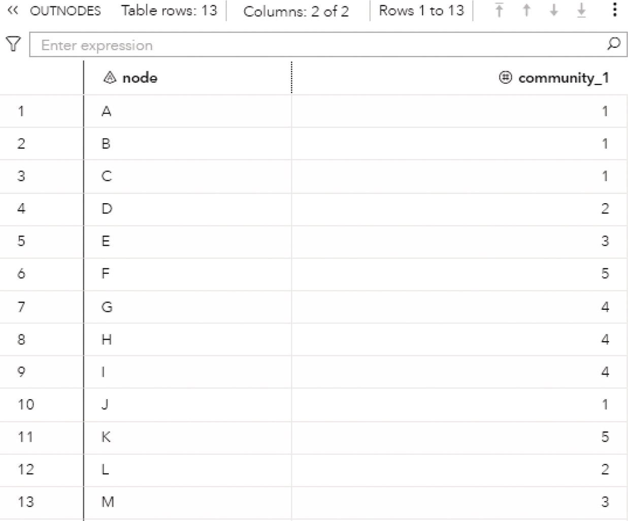
Figure 2.43 Output nodes table for the community detection.
The following code shows how to invoke the parallel label propagation algorithm for the directed graph. Differently than the label propagation algorithm, the parallel label propagation can use a list of resolutions when detecting the communities. The difference between the Louvain algorithm and the parallel label propagation is that the first one executes all resolutions at the same time, and the second executes each resolution one at a time. Here we are using one single resolution, 1.0.
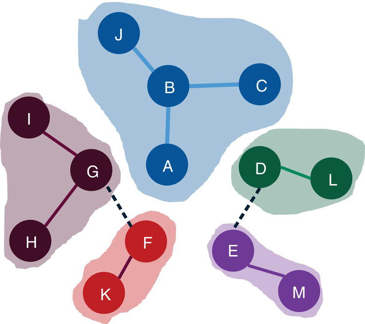
Figure 2.44 Communities identified by the label propagation algorithm with the recursive option.
proc networkdirection = directedlinks = mycas.linksoutlinks = mycas.outlinksoutnodes = mycas.outnodes;linksvarfrom = fromto = to;communityalgorithm=parallellabelpropresolutionlist = 1.0outlevel = mycas.outcommleveloutcommunity = mycas.outcommoutoverlap = mycas.outoverlapoutcommLinks = mycas.outcommlinks;run;
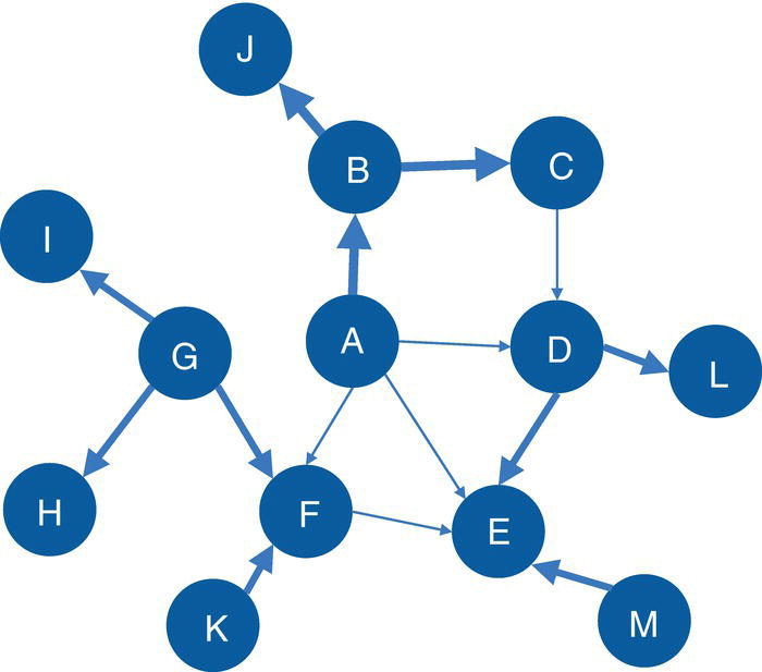
Figure 2.45 Input graph with directed weighted links.
The OUTCOMMLEVEL table presented in Figure 2.46 shows the final result for the community detection based on the parallel label algorithm upon a directed graph. This execution identified 3 communities. The modularity of 0.3 is the lowest considering all algorithms used before.
The OUTNODES table presented in Figure 2.47 shows the distribution of the nodes throughout the communities. Based on a directed graph, nodes A, C, B, and J form the community 1, nodes E, I, M, D, L, G, K, and F form community 2, and node H is isolated in community 3.
Figure 2.48 shows the final community topology for the parallel label propagation algorithm based on a directed graph, highlighting the 3 communities detected.
As we can see, different algorithms can detect distinct communities. The direction of the graph also plays a critical role, causing the algorithms to identify different topologies. As an optimization algorithm, different executions may end up with different results, particularly on large networks.
Finally, let's see two additional methods that can be used during the community detection process. The first method forces nodes to be in the same community at the beginning of the recursive partitioning. These nodes defined to be in the same community at the beginning of the recursive partitioning can definitely interchange communities throughout the execution. The second method forces nodes to be in the same community at the end of the partitioning process.
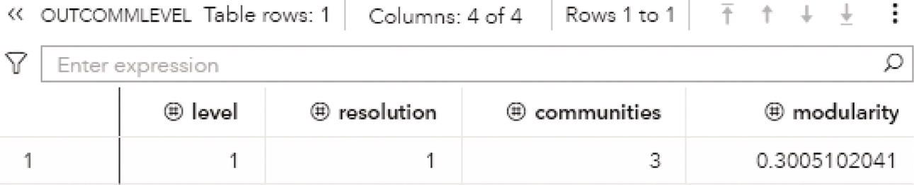
Figure 2.46 Output communities' level table for the community detection.
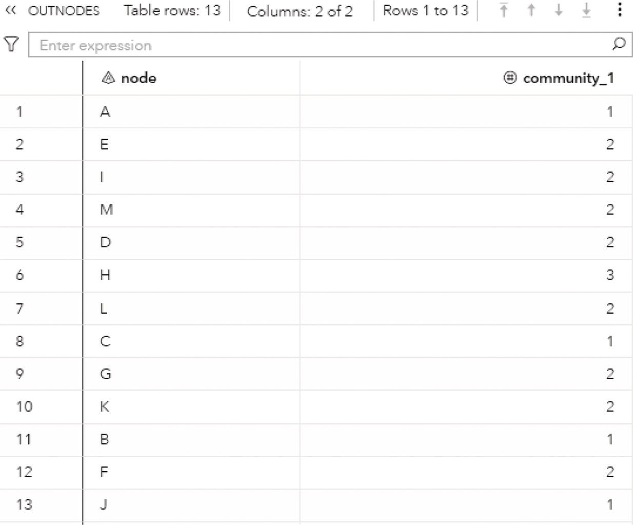
Figure 2.47 Output nodes table for the community detection.
The first part of the following code defines the set of nodes that needs to be in the same community at the beginning of the recursive partitioning process. Nodes A, L, E, and M need to be in the same community at the beginning of the community detection. The variable warm defines the community identifier for the nodes at the beginning of the process. In this example, all nodes have the value 1, indicating that they will start all together at the same community. We can define multiple sets of nodes by specifying different values for the variable warm. For example, nodes A and B with warm value 1, nodes C and D with warm values equal to 2, and nodes E and F with warm value 3. In this case, the first partitioning step considers nodes A and B in the same community, as well as nodes C and D and nodes E and F. They can change communities throughout the partitioning process and can end up in different communities at the final topology.
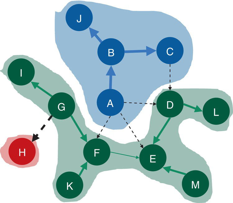
Figure 2.48 Communities identified by the parallel label propagation algorithm based on a directed input graph.
data mycas.nodeswarm;input node $ warm @@;datalines;D 1 L 1 E 1 M 1;run;
The following code invokes the community detection algorithm considering an initial set for nodes D, L, E, and M. The set of nodes used at the beginning of the recursive partitioning are specified by using the option NODES = in the NETWORK statement. The initial communities for the warm nodes are specified by using the option WARMSTART = in the COMMUNITY statement. The warm variable created in the nodes' dataset definition is referenced in that option.
proc networkdirection = undirectednodes = mycas.nodeswarmlinks = mycas.linksoutlinks = mycas.outlinksoutnodes = mycas.outnodes;linksvarfrom = fromto = to;nodesvarnode = node;communitywarmstart=warmalgorithm=labelpropresolutionlist = 1.0outlevel = mycas.outcommleveloutcommunity = mycas.outcommoutoverlap = mycas.outoverlapoutcommLinks = mycas.outcommlinks;run;
The OUTCOMMLEVEL table presented in Figure 2.49 shows the final result for the community detection based on the label algorithm using a warm set of nodes to initiate the recursive partitioning. This execution identified 3 communities. The final modularity is around 0.5915.
The OUTNODES table presented in Figure 2.50 shows the distribution of the nodes in different communities based on a warm start. Nodes A, B, C, and J form the community 2, nodes D, E, L, and M form community 3 and nodes F, G, H, I, and K form community 1.
Notice that the warm process started with nodes D, L, E, and M. A previous execution of the label propagation algorithm with resolution 1.0 ended up with four communities, where nodes D and L formed one community and nodes E and M formed another one. Now, because of the warm start, only three communities were found, and nodes D, L, E, and M ended up in the same community.
Figure 2.51 shows the final result for the label propagation algorithm using the warm start for the community detection.
They could have ended up in different communities as the warm start only forces nodes to initiate the recursive partitioning, not finish at the same community.
The method to force a set of nodes to finish at the same community is applied by using the option FIX =. The following code creates the nodes dataset with the community identifier for each one of them. For example, nodes D and L are set to end up at the same community, and nodes F and E are set to end up at another one. The first set is defined by the value 1 for the variable fixcomm, and the second set is defined by the value 2. Many different sets can be defined in the nodes' dataset definition.
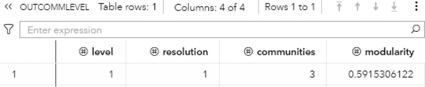
Figure 2.49 Output communities' level table for the community detection.
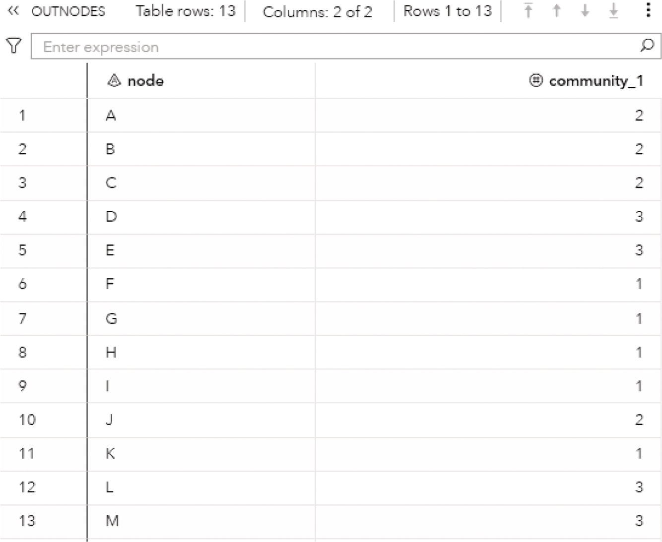
Figure 2.50 Output nodes table for the community detection.
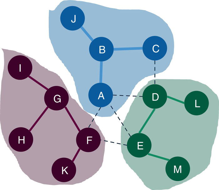
Figure 2.51 Communities identified by the label propagation algorithm with the warm start.
data mycas.nodesfix;input node $ fixcomm @@;datalines;D 1 L 1F 2 E 2;run;
The following code invokes the community detection algorithm considering the nodes that are fixed to end up in the same communities. The set of nodes are set by using the option NODES = in the NETWORK statement. The final communities for the fixed nodes are specified by using the option FIX = in the COMMUNITY statement. The variable fixcomm specified in the nodes' dataset definition is referenced in the FIX = option.
proc networkdirection = undirectednodes = mycas.nodesfixlinks = mycas.linksoutlinks = mycas.outlinksoutnodes = mycas.outnodes;linksvarfrom = fromto = to;nodesvarnode = node;communityfix=fixcommalgorithm=labelpropresolutionlist = 1.0recursive(maxcommsize=4 maxdiameter=3 relation=and)outlevel = mycas.outcommleveloutcommunity = mycas.outcommoutoverlap = mycas.outoverlap;run;
The OUTCOMMLEVEL table presented in Figure 2.52 shows the final result for the community detection based on the label algorithm using a fixed set of nodes ending up in the same communities. This execution identified 4 communities. The final modularity is around 0.5277.
The OUTNODES table presented in Figure 2.53 shows the distribution of the nodes throughout the communities. Based on the sets of fixed nodes, nodes A, C, B, and J form the community 1; nodes D and L form community 3; as defined in the fixed nodes option; nodes E, F, K, and M form community 4; having nodes F and E in the same community as defined in the fixed nodes option; and nodes G, H, and I form the final community 2.
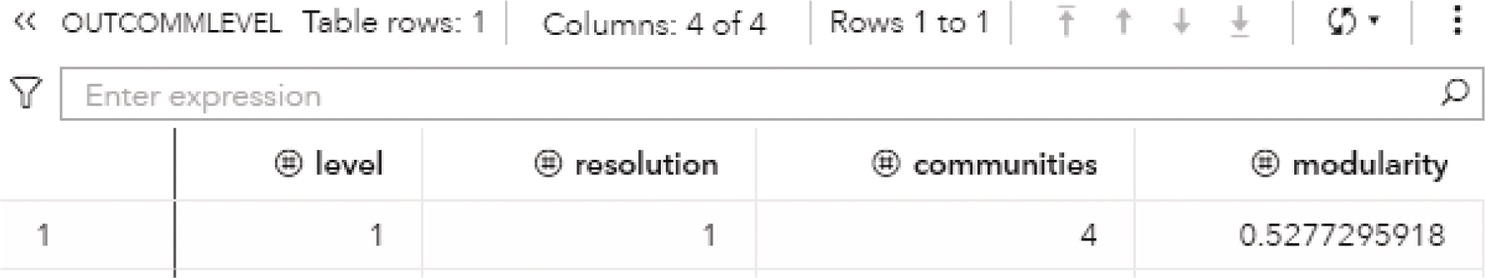
Figure 2.52 Output communities' level table for the community detection.
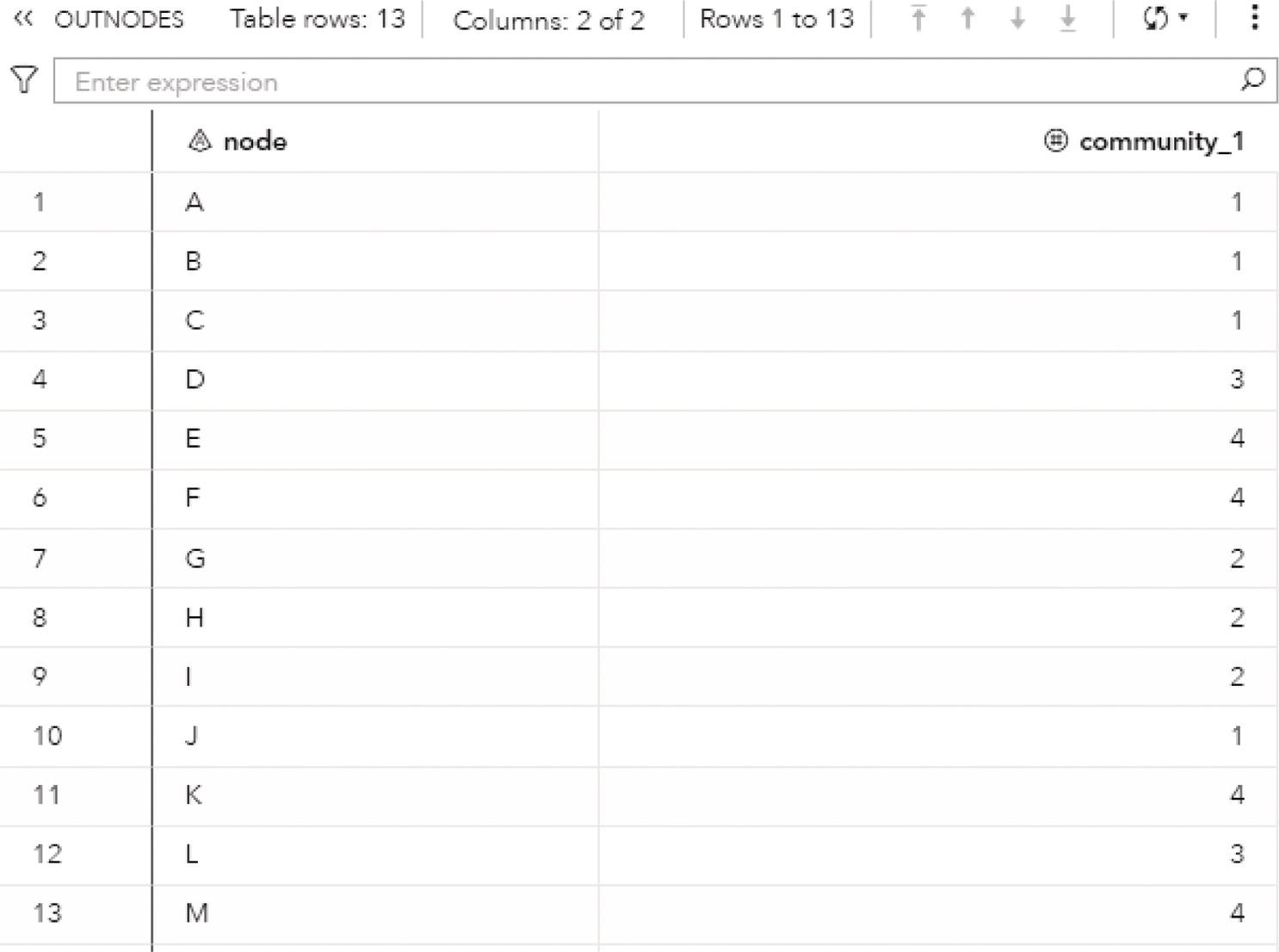
Figure 2.53 Output nodes table for the community detection.
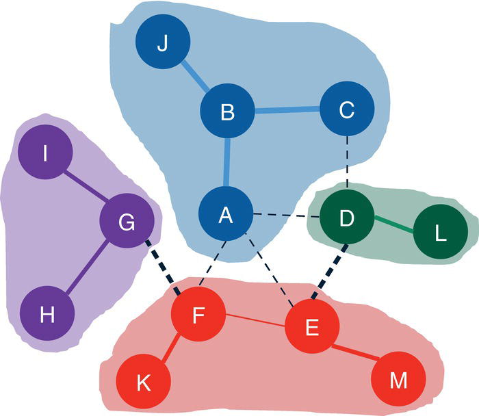
Figure 2.54 Communities identified by the label propagation algorithm with the fixed nodes.
Figure 2.54 shows the final result for the label propagation algorithm using the fixed nodes for the community detection process.
Notice that the regular execution with the label propagation algorithm ended up with nodes D and L forming a unique community, as defined for one set of fixed nodes. However, the node F ended up in a community with nodes I, G, H, and K, and node E ended up in a community with node M. As the nodes F and E were fixed to be in the same community and based on the sum of the link weights between the nodes, nodes F, E, K, and M ended up in one community, and nodes I, G, and H were set in a different one.
There are many methods and approaches to detecting communities, especially in large networks. Most of the time, the process is iterative, based on executions and post analyzes. As stated before, modularity is commonly used to select the best community topology among several executions and upon different resolutions. Recursive methods to limit the size of each community and the average distance between the nodes within the same community are also used in order to mitigate large partitions. A combination of algorithms like Louvain and label propagation are also possible to narrow down the selection process of the best community topology. Often, the Louvain algorithm can be executed on multiple resolutions, and the label propagation can be later executed using the best resolution and the recursive options. Also, even though the network is represented by a directed graph, in some cases the execution of Louvain or label propagation on an undirected graph can make sense and produce better results. The network metrics can still be computed based on the directed links even though the communities are identified based on undirected connections. Finally, business context and the domain knowledge can be used in the process to identify the best community topology according to the particular goal and the problem definition. There is no right or wrong in community detection. The best community distribution may vary according to multiple variables and different scenarios.
2.5 Core
A k‐core decomposition is an undirected graph where every subgraph has nodes with degree at most k. In other words, some nodes in the subgraphs are linked to k or less other nodes throughout the subgraphs' links. A k‐core of an undirected graph can also be seen as the maximal connected component of the graph G where all nodes have degree at least k.
K‐core decomposition has many applications in multiple industries, like pharmaceutical companies, information technology, transportation, telecommunications, public health, etc., along various disciplines such as biology, chemistry, epidemiology, computer science, social studies, etc. It is commonly applied to visualize network structures, to interpret cooperative connections in social networks, to capture structural variety in social contagion, to analyze network hierarchies, among many others.
The core algorithm finds cohesive groups within a network by extracting k‐cores. It can be seen as an alternative process for community detection. The core decomposition is not as powerful as the community detection algorithms in searching groups of nodes based on the strength of their relationships, but it can find a rough approximation of cohesive structures within the network with a low computational cost.
The core of a graph G = (N, L) is defined as an induced graph on nodes S, where G S = (S, L S ).
The subgraph G S is a k‐core only if every node in S has a degree centrality greater than or equal to k, and G S is the maximum subgraph with this property.
An important concept assigned to the k‐core decomposition is that all the cores found in a network are nested. For example, if ![]() is a k‐core of size k, then
is a k‐core of size k, then ![]() is contained in
is contained in ![]() .
.
In proc network, the CORE statement invokes the k‐core decomposition algorithm. This algorithm determines the core hierarchy considering a straightforward property. From a given graph G = (N, L) it recursively deletes all nodes and links incident with them, of degree less than k. The remaining graph is the k‐core.
The final results for the core decomposition algorithm in proc network are reported in the output nodes data table specified by the option OUTNODES =. The k‐core decomposition algorithm can be executed based on undirected and directed graphs. For an undirected graph, each node in the output nodes data table is assigned to a core through the variable core_out, which identifies the core number, and the highest‐order core that contains this node. For a directed graph, each node in the output nodes data table is assigned to a core‐in and core‐out through the variables core_in and core_out, respectively.
The only option for the CORE statement is the MAXTIME = option. This option specifies the maximum amount of time to spend calculating the core decomposition. The type of time (either CPU time or real time) is determined by the value of the TIMETYPE = option in the PROC NETWORK statement. The default is the largest number that can be represented by a double.
Let's see an example of k‐core decomposition in both directed and undirected graphs.
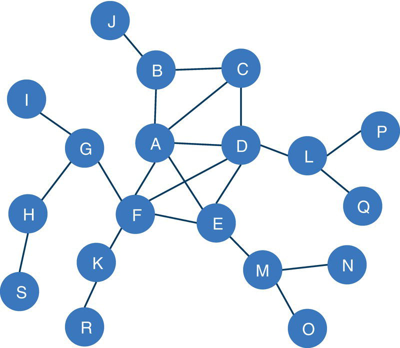
Figure 2.55 Input graph with undirected links.
2.5.1 Finding k-Cores
Let's consider the following graph to demonstrate the k‐core decomposition algorithm. This graph is an extension of the graph used previously to demonstrate the community detection algorithm. It has 19 nodes and 23 links, slightly larger than the previous one. Also, the link weights in k‐core decomposition are not necessary and then they were suppressed from the links dataset. Figure 2.55 shows the input undirected graph.
The following code creates the input dataset for the k‐core decomposition algorithm. The links dataset contains only the origin and destination nodes.
data mycas.links;input from $ to $ @@;datalines;A B B C B J A F A E A D A C C DF D F E G F G I G H K F D L D EM E M N M O L P L Q K R H Srun;
Once the input dataset is created, we can now invoke the k‐core decomposition algorithm using proc network. The following code describes how to do that. In the LINKSVAR statement, the variables from and to receive the origin and the destination nodes, even though the direction is not used at this first run. The final result for the k‐core decomposition is reported in the output table defined by the OUTNODES = option.
proc networkdirection = undirectedlinks = mycas.linksoutnodes = mycas.outnodes;linksvarfrom = fromto = to;core;run;
The following pictures show the outputs for the k‐core decomposition algorithm. Figure 2.56 reports the summary for the execution process. It provides the size of the network, with 19 nodes and 23 links, and the direction of the graph, the algorithm executed (the problem type) and the output tables.
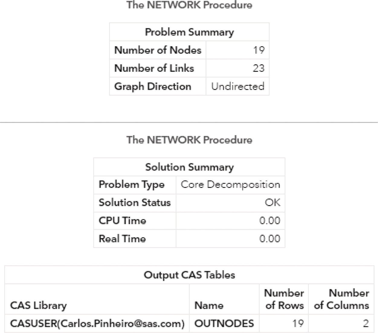
Figure 2.56 Output summary results for the k‐core decomposition on an undirected graph.
The OUTNODES table presented in Figure 2.57 shows each node within the network and which core it belongs to.
Notice that the nodes in the same core don't necessarily need to have the same degree. As nested or hierarchical cores, nodes in the same k‐core need to have a degree greater than or equal k. For example, based on the previous undirected input graph, it starts from the less cohesive cores to the most cohesive ones. Starting off with core 1, all nodes must have a degree greater than or equal 1. This is the case for nodes J, I, S, R, O, N, Q, and P with degree of 1, node K with degree of 2, and nodes G, M, and L with degree of 3. They all fall into core 1. Core 2 comprises nodes B and C with degree of 3. The question here is why nodes G, M, and L, which also have degree of 3 are not in the same core 2? The answer is because they are not connected. Core is a matter of interconnectivity, which accounts for the degree of connections but also the existing connections among nodes. Finally, core 3, the most cohesive one, has nodes A, D, and F with degree of 5 plus node E with degree of 4.
Figure 2.58 shows the nested cores highlighted.
Let's see how the k‐core decomposition works on directed graphs. In addition to the interconnectivity, the k‐core decomposition in directed graphs also takes into consideration the information flow created by the directed links.
Let's use the same graph defined previously. The direction of the links will follow the definition of the links data set. For example, the definition of the link A B means will create a directed link A→B.
The code to execute the k‐core decomposition is exactly the same as used before, except by the DIRECTION = option, which will be specified as DIRECTED. The following code line shows the definition.
direction = directed
The method to find cores within directed graphs is basically a search for circuits, as the directed links create unique paths within the network.
Based on the current links set, the original input graph has one single core, as shown by the output table OUTNODES presented in Figure 2.59.
Notice that as a directed graph, two core identifiers are provided, the core_out and the core_in variables. Both identifiers in these examples are zero, representing that the entire network is a single core.
Let's change one single direction in the original input graph, switching the link A→D to the link D→A. Now, two cores are identified. There are two sets of nodes identified by the core out, and a different two sets of nodes identified by the core in. Figure 2.60 shows the output table OUTNODES.
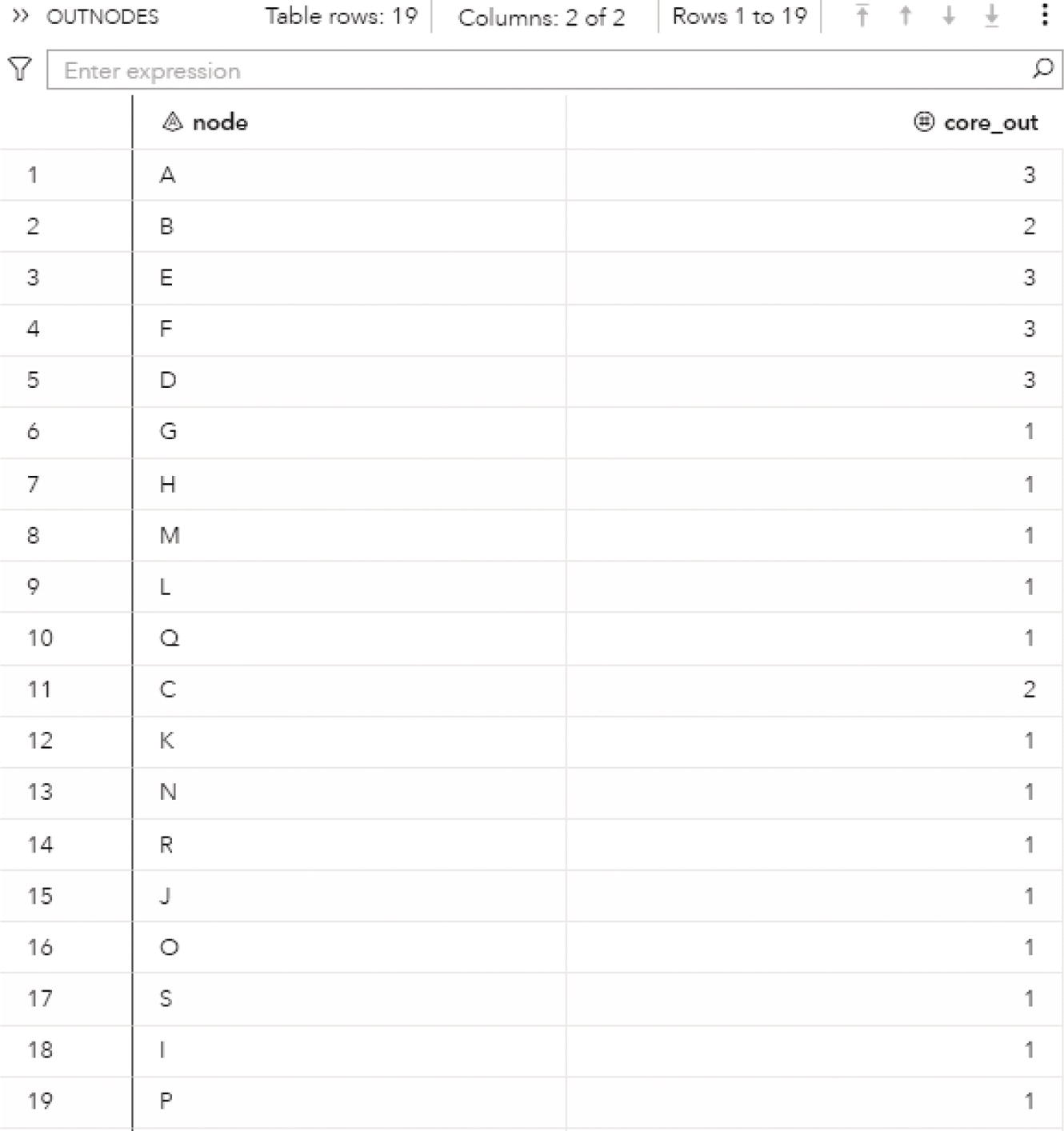
Figure 2.57 Output for the k‐cores and the assigned nodes.
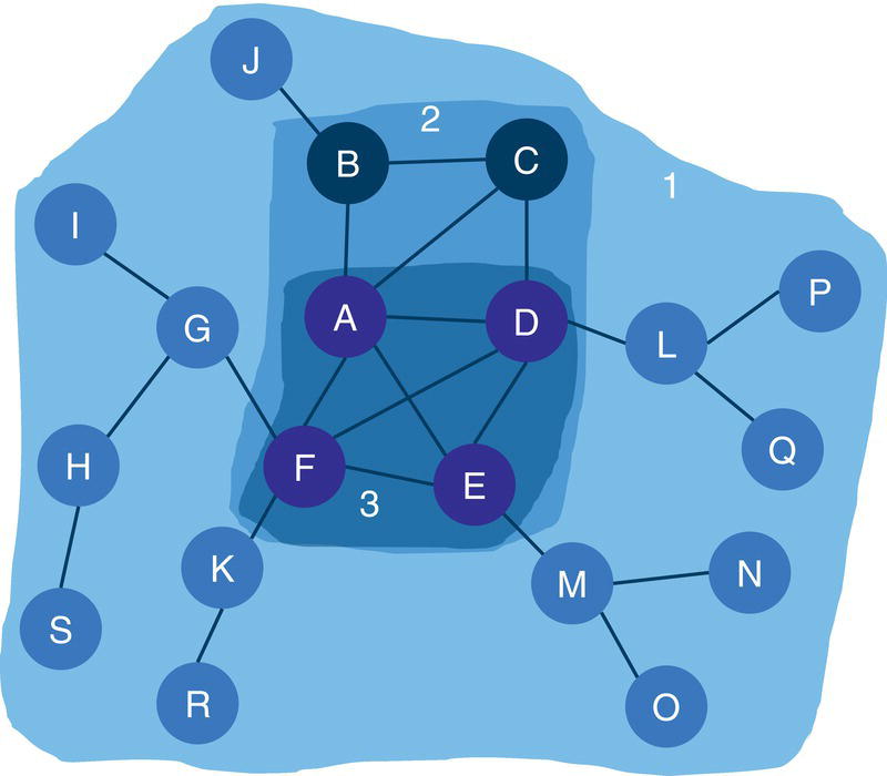
Figure 2.58 The undirected input graph highlighting the cores and the nodes for each core.
Based on the core out, nodes A, B, C, D, F, G, and K fall into core 1. Based on the direction of the links between them, a circuit comprising nodes A, B, C, and D is found. Nodes K, G, and F can reach out to this circuit. They all form the core out 1.
Figure 2.61 shows the two cores based on the core out identifier. The direction of the links is shown, and the link that has the directed switched is highlighted.
Based on the core in, there are also two cores, but the set of nodes in each one of them is different than the sets based on core out. Now, nodes A, B, C, D, E, F, J, L, P, and Q fall into the same core in. Similarly, there is a circuit between nodes A, B, C, and D, but now nodes F, E, J, L, P, and Q can be reached from that circuit. They all form the core in 1. Figure 2.62 highlights this core within the directed graph.
Notice that many algorithms in network analysis, particularly in terms of subgraph detection, are intended, or at least designed to be undirected graphs. That is the case for connected components, biconnected components, community detection, and k‐core decomposition. However, there are algorithms available to compute the same type of subgraphs considering directed graphs. The main distinction between them is that a directed graph has unique paths among nodes, which changes the information flow throughout the network.
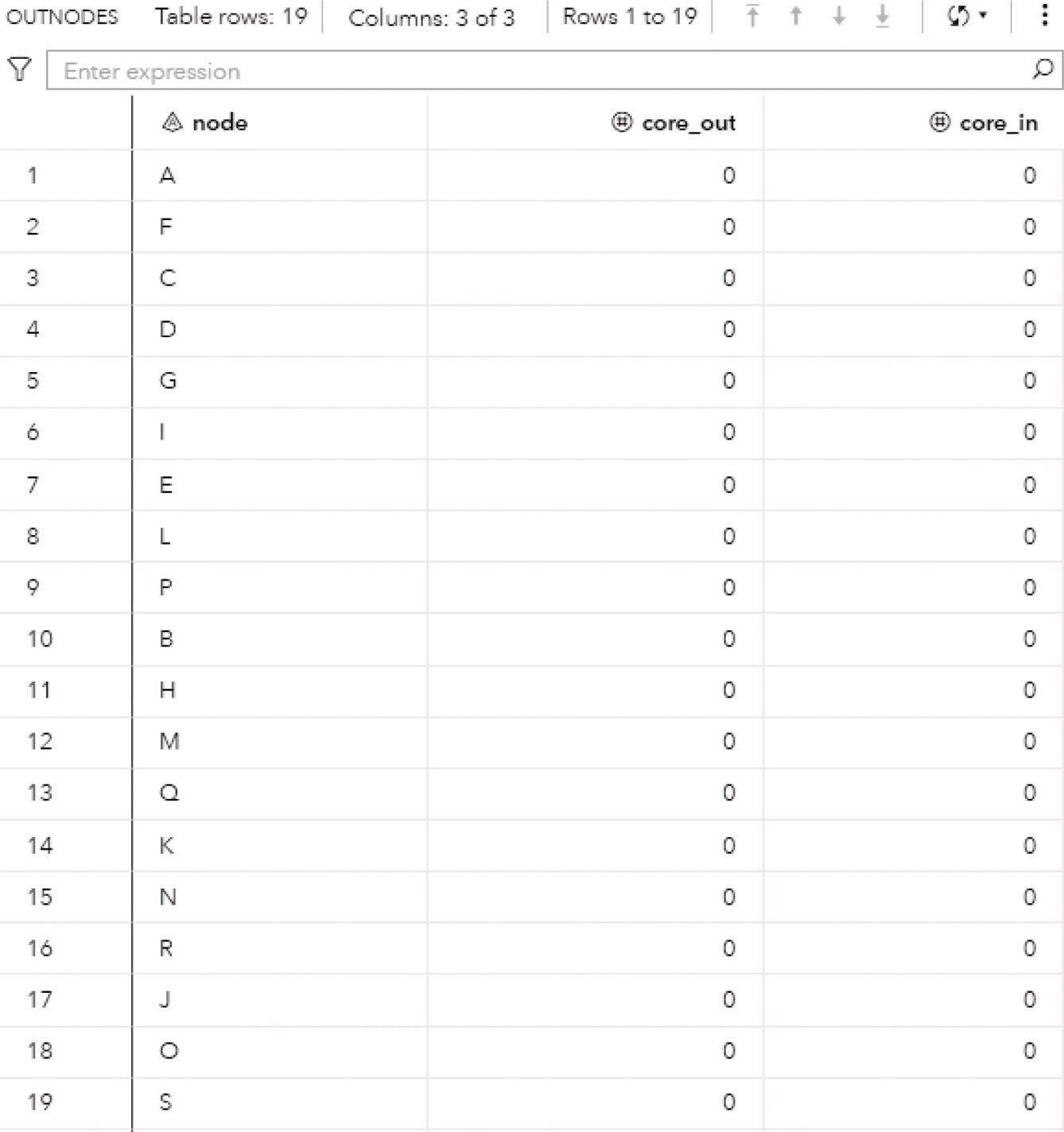
Figure 2.59 Cores identified by the k‐core decomposition algorithm.
2.6 Reach Network
Reach networks, also known as ego or egocentric networks, focus on the analysis of groups of nodes based on a particular set of nodes, or a single node. This method considers the individual node, or a set of nodes, rather than the entire structure of the network. The node starting the analysis is referred to as the ego, or in the case of a set of nodes, each node in the initial set will create an ego network. All connections of the ego nodes are captured and analyzed in order to identify the related nodes, and therefore, create its neighborhood, or its particular subnetwork. The analysis of the connections incident to the ego nodes is important to highlight how the subnetwork can affect the ego nodes, but mostly how the ego nodes can affect the rest of the subnetwork. Often, the ego nodes are selected based on their network centralities. The more connected, or more central nodes, are targeted as ego nodes and the reach network is computed. This approach normally highlights possible viral effects or cascade events throughout the network over time, which is especially useful in marketing, sales, and relationships campaigns, but also in fraud detection processes. The analysis concentrates on how many nodes the ego nodes can reach out, considering one single connection or degree of separation, or eventually more connections (second degree, third degree, and so forth). In reach networks, the focal or initial nodes are called ego, and the links incident to the egos are called alters.
Although the structure created by the ego network does not represent the entire network, egocentric data can be particularly important in network analysis. Particularly in large networks, this method is useful in understanding some subgraphs features or some specific social structures within the entire network. Very often, the analysis of the ego networks reveals possible influencers and how wide they can affect their social structures. The influencers, or the ego nodes, varies depending on the context or problem. They can be customers, companies, organizations, countries, etc. Therefore, their particular ego networks can represent a company's market or customer base, business relations, or international trading between countries or organizations, and financial transactions, among many others.
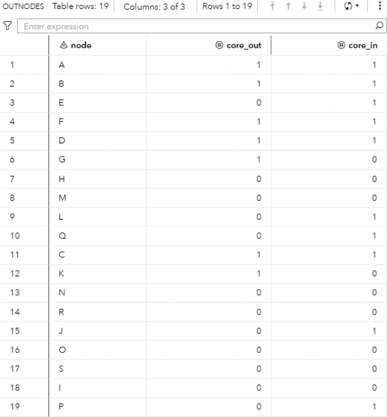
Figure 2.60 Cores out identified by the k‐core decomposition algorithm.
In some specific applications such as financial risk, fraud events, etc., the ego networks can expose a possible viral effect of an illegal transaction or operation. Once an entity (company, group, individual) is identified as committing fraud, the ego network associated with that entity indicates how wide the illegal actions can be. Additional suspicious actors, especially in fraud, can be highlighted by the analysis of the ego networks. Particularly in fraud, in most cases, the business scenario consists of an entire structure behind the scenes to make it work. Beginning by looking at a small set of individuals or entities can be beneficial in narrowing down the fraud detection process exposing other actors that might be involved.
Formally, the reach network of a graph G = (N, L) is defined as a subgraph ![]() , induced by the set of nodes
, induced by the set of nodes ![]() that are reachable in H steps or hops from a set of nodes S called source nodes. Reach network can be executed in both undirected and directed graphs. Particularly for directed graphs, the set of nodes
that are reachable in H steps or hops from a set of nodes S called source nodes. Reach network can be executed in both undirected and directed graphs. Particularly for directed graphs, the set of nodes ![]() that can be reached by the set of source nodes S is identified by using only the outgoing links. The induced subgraph created by the outgoing links is often called the out‐reach network.
that can be reached by the set of source nodes S is identified by using only the outgoing links. The induced subgraph created by the outgoing links is often called the out‐reach network.

Figure 2.61 Cores out highlighted in the directed network.
In proc network, the REACH statement invokes the algorithm to identify the ego networks within the network starting from an initial set of ego nodes. There are two methods to define this initial set of ego nodes. Commonly, the set of ego nodes used to compute the reach networks are defined in the data table consisting of a subset of nodes. The NODESSUBSET = option specifies that particular subset of ego nodes. This option to define a subset of nodes to begin an algorithm can be used to find the reach network, but also to the algorithms to find paths, shortest paths, and nodes similarity. The data table used to specify the initial set of ego nodes can define distinct sets of sources nodes. Each set of source nodes is used to find one specific reach network. For example, suppose we are interested in three distinct groups of nodes, and we want to evaluate the reach network of each one of these three sets. Then, in the data table used to define the ego nodes (the nodes subset) we can specify the nodes and the subset they belong to. The alternative method to compute the reach network is to specify all nodes. The option EACHSOURCE determines that proc network will search the reach network for all nodes within the network, or the nodes presented in the links dataset.
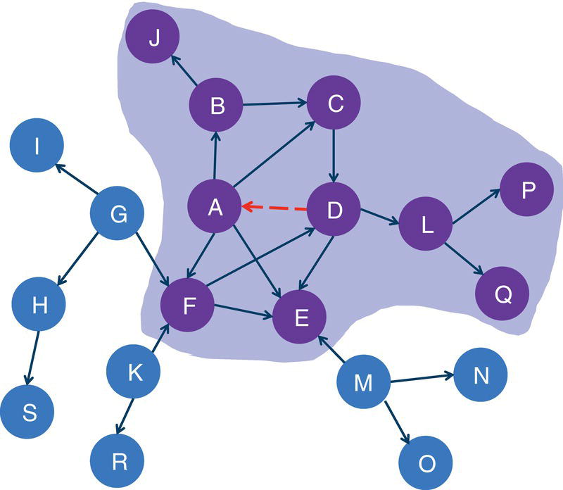
Figure 2.62 Cores in highlighted in the directed network.
The number of steps from the ego node, or the source node, to the related node, or the sink node, can also be determined when proc network computes the reach network for each subset of ego nodes. For example, we can define that the reach network for a particular ego node will consider the straight connected nodes, or the straight connected nodes plus the nodes connected to them. The first case represents a reach of 1, and the second case represents a reach of 2. As we increase the maximum reach, the ego network produced by the algorithm can be quite large. The outcome from the reach network algorithm, especially considering a large network and a great amount of ego nodes can be computationally intensive.
The final results for the reach network algorithm in proc network are reported in the output tables defined by the options OUTREACHNODES =, OUTREACHLINKS =, and OUTCOUNTS =. These output tables may contain several columns, may vary according to the direction of the graph, and whether the nodes have weights defined in the dataset representing the nodes.
The OUTREACHNODES = option defines the output table containing the nodes of each reach network associated with all subsets of ego nodes specified in the NODESSUBSET = option. This output contains the following columns:
- Reach: the identifier of the reach network associated with each subset of source nodes.
- node: the label of the node for each node in each reach network.
The OUTREACHLINKS = option defines the output table containing the links of each reach network associated with all subsets of ego nodes specified in the NODESSUBSET = option. This output contains the following columns:
- reach: the identifier of the reach network associated with each subset of source nodes.
- from: the label of the from node for each link in each reach network.
- to: the label of the to node for each link in each reach network.
The OUTCOUNTS = option defines the output table containing the number of nodes of each reach network associated with all subsets of ego nodes specified in the NODESSUBSET = option. This output contains the following columns:
- reach: the identifier of the reach network associated with each subset of source nodes.
- node: the label of the node for each node in each reach network.
- count: the number of nodes in the (out‐)reach network from the subset of source nodes.
- count_not: the number of nodes not in the (out‐)reach network from the subset of source nodes.
As we noticed before, nodes and links can be weighted in order to represent their importance within the network. For the reach algorithm, if the nodes have weights, the output table specified by the option OUTCOUNTS = contains some additional columns:
- count_wt: the sum of the weights of the nodes counted in the (out‐)reach network.
- count_not_wt: the sum of the weights of the nodes not counted in the (out‐)reach network.
The reach network can be computed for both directed and undirected graphs. For a directed graph, proc network has an option to compute the direct counts when the number of steps from the source node and the sink node is limited to 1. In that case, the output table specified by the option OUTCOUNTS = contains some additional columns:
- count_in: the number of nodes that reach some node in the subset of source nodes using at most one step.
- count_out: the number of nodes in the out‐reach network from the subset of source nodes.
- count_in_or_out: the number of nodes in the union of the subset of nodes counted in count_in and count_out.
- count_in_and_out: the number of nodes in the intersection of the subset of nodes counted in count_in and count_out.
In the case of the defined weight of the nodes, and the directed graph, the output table defined by the option OUTCOUNTS = contains more additional columns:
- count_in_wt: the sum of the weights of the nodes counted in count_in.
- count_out_wt: the sum of the weights of the nodes counted in count_out.
- count_in_or_out_wt: the sum of the weights of the nodes counted in count_in_or_out.
- count_in_and_out_wt: the sum of the weights of the nodes counted in count_in_and_out.
As mentioned before, if the network has directed links, it is possible to compute the number of directed counts for each reach network. The option DIGRAPH forces proc network to calculate the directed reach counts when computing the reach networks. The directed counts are reported in the output table specified in the option OUTCOUNTS =. The directed counts are calculated when the graph is directed, and the maximum reach is 1.
The option EACHSOURCE treats each node in the network as a source node (ego node), and then calculates the reach network from each node in the input graph. For a large network, this option can be computationally intensive. The output results when using this option in large networks can also be extremely large. This is the second method to define the source nodes when computing the reach networks. Often, a subset of nodes is defined, including the possibility of specifying distinct sets of source nodes, and then the option NODESSUBSET = is used.
The option MAXREACH = specifies the maximum number of steps from each source node in a reach network. For example, MAXREACH = 1 specifies that all nodes directed connected to a source node are counted in the reach network. MAXREACH = 2 add to the reach network all nodes linked to the nodes connected to that source node. The default for the option MAXREACH = is 1.
Let's see some examples of reach networks for both directed and undirected graphs.
2.6.1 Finding the Reach Network
Let's consider a graph similar to the one used to demonstrate the k‐core decomposition, presented in Figure 2.63. This graph has 12 nodes and 12 links. Initially this graph will be considered an undirected graph, with no link weights.
The following code describes the creation of the links dataset and the subset of ego or source nodes. The reach algorithm will use each subset of source nodes to compute the different reach networks. The links dataset has only the nodes identification, specified by the from and to variables. There are two subsets of ego nodes. The first one has just node A, identified by the variable reach equals 1, and the second subset contains nodes D and G, identified by the variable reach equals 2.
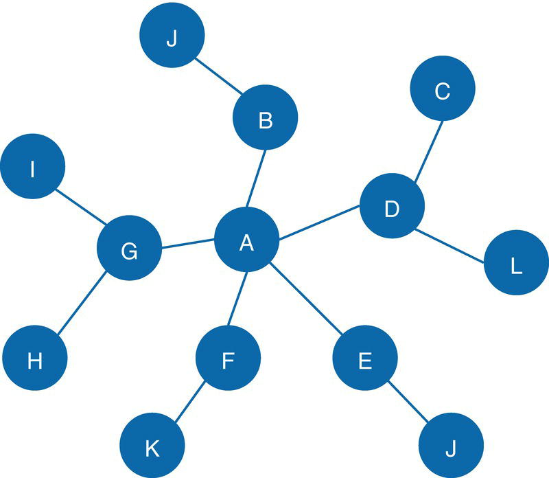
Figure 2.63 Input graph with undirected and unweighted links.
data mycas.links;input from $ to $ @@;datalines;A B B J A G G I G H A D D C D L A F F K A E E J;run;data mycas.egonodes;input node $ reach @@;datalines;A 1 G 2 D 2;run;
Once the input links dataset is defined, we can invoke the reach network algorithm in proc network. The following code describes the process. Notice the links definition using the LINKSVAR statement. Also notice the NODESSUBSET option to define the subsets of ego nodes to start off the reach network computation. All three possible output tables are specified, for links, nodes, and counts.
proc networkdirection = undirectedlinks = mycas.linksnodessubset = mycas.egonodes;linksvarfrom = fromto = to;reachoutreachlinks = mycas.outreachlinksoutreachnodes = mycas.outreachnodesoutcounts = mycas.outreachcounts;run;
Figure 2.64 shows the summary output for the reach network algorithm. It shows the size of the network, (12 nodes and 12 links), the direction of the graph, the algorithm used, the time to process, and the final output tables.
The OUTREACHNODES table presented in Figure 2.65 shows all reach networks and the nodes on them. The variable reach identifies the reach network, and the variable node identifies which node belongs to each reach network.
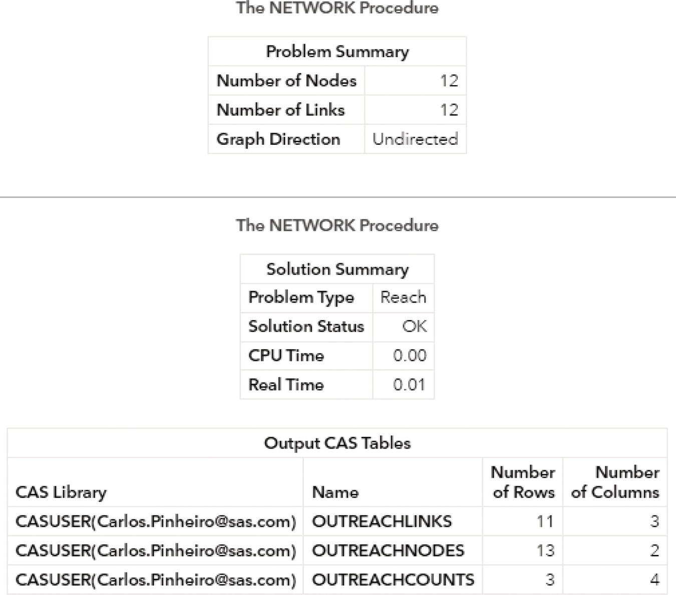
Figure 2.64 Output results by proc network running the reach network algorithm on an undirected graph.
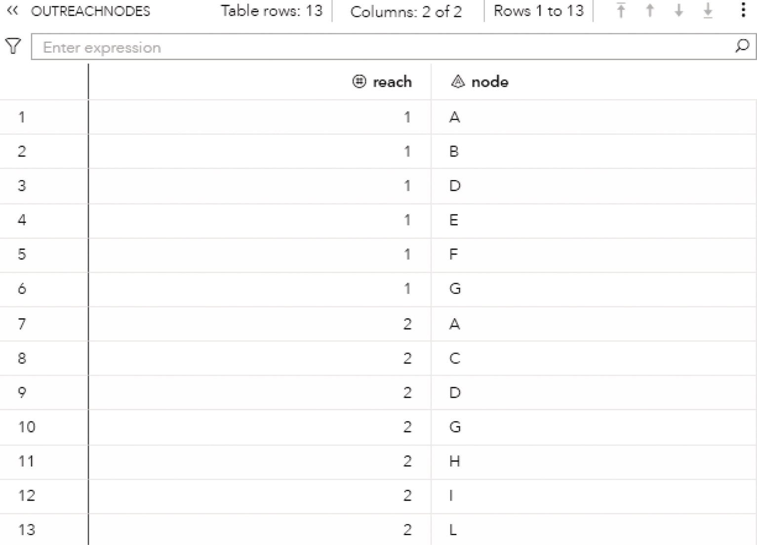
Figure 2.65 Output nodes table for the reach network.
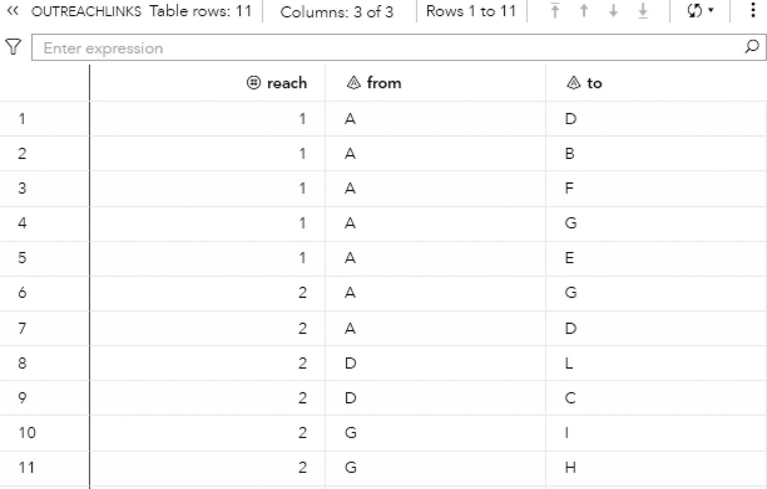
Figure 2.66 Output links table for the reach network.
Notice that there are two subsets of nodes. The first one comprises only the node A. Its reach network consists of node A, of course, plus nodes B, D, E, F, and G. The second subset of ego nodes comprises nodes D and G. The second reach network consists of nodes D and G, plus nodes A, I, H, C, and L.
The OUTREACHLINKS table presented in Figure 2.66 shows the links within each reach network identified.
Finally, the OUTCOUNTS table presented in Figure 2.67 shows the number of nodes in each reach network by each ego node. It shows the number of nodes within the reach network and also the number of nodes outside the ego network.
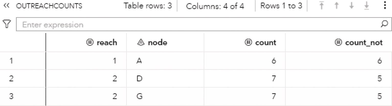
Figure 2.67 Output links table for the reach network.
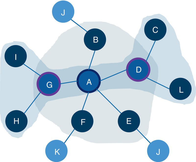
Figure 2.68 Input graph with the reach networks highlighted.
For example, the reach network 1, based on the ego node A, has 6 nodes within it and 7 nodes outside of it. The reach network 2, based on the ego nodes D and G, has 7 nodes within it and 5 nodes outside of it.
Figure 2.68 shows a graphical representation of the two reach networks.
The MAXREACH = option plays an important role when computing the reach network. Depending on the level of connectivity of the network, a high maximum reach can represent a large ego network. For example, using this small network, let's increase the maximum number of steps of hops from 1 to 2. Let's use just node A as the source node. The subset node would contain only node A.
data mycas.egonodes;input node $ reach @@;datalines;A 1;run;
Also, the option MAXREACH = needs to be set within the proc network.
proc network...reachmaxreach = 2...run;
Because of the small size and of the high connectivity network, the ego network of node A considering 2 hops is the entire network. The OUTREACHCOUNTS table presented in Figure 2.69 shows the count for the reach network assigned to node A. All 12 nodes within the network were counted.
The use of the EACHSOURCE option forces proc network to compute the reach network for all nodes in the network. For large networks, the time to compute all reach networks as well as the size of the output can be extremely large. This option must be used with caution. The following code shows only the part of the REACH statement including the EACHSOURCE option.
proc network...reacheachsource...run;
The OUTREACHCOUNTS table presented in Figure 2.70 shows the counts for all reach networks. Notice that all 12 nodes in the original network are represented there.
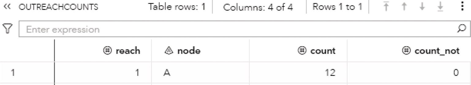
Figure 2.69 Counts table for the node A using maximum reach equals 2.
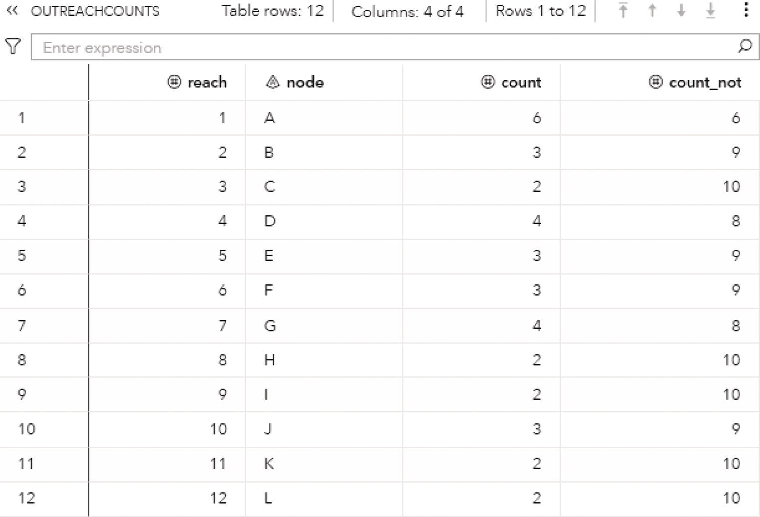
Figure 2.70 Counts for all reach networks considering all nodes as source.
Finally, the direction of the link plays a crucial role when computing reach networks. The paths created by the directed links are considered to assess when a sink node can be reached out by a source node. For example, using the same network, let's just invert the definition of two links, from the original D→C and D→L, to C→D and L→D. Let's also use only node D as the ego node. See the following parts of the code to proceed with these changes.
data mycas.links;input from $ to $ @@;datalines;... C D L D ...;run;data mycas.egonodes;input node $ reach @@;datalines;D 1;run;proc networkdirection = directed...run;
Figure 2.71 shows the portion of the network with the two directed links.
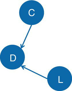
Figure 2.71 Directed links for node D.
The OUTREACHCOUNTS table presented in Figure 2.72 shows the reach network for node D. Notice that there is only 1 count for it, which is node D itself. Nodes C and L, previously counted in its ego network on the undirected graph are not counted now because node D cannot reach out to nodes C and L.
The additional columns in the outputs when the links and nodes are weighted are suppressed here because they actually don't change the search for reach network. They do change the outcomes by adding all weight information in the output tables.
2.7 Network Projection
Bipartite graphs are graphs with two distinct partitions of nodes. The nodes assignment is mutually exclusive, which means nodes must be assigned to one partition or the other. In unipartite graph, all nodes and links within the network belong to the same set or partition. This single set or partition contains unique nodes and links. Neither nodes nor links can be duplicated in the network. In bipartite graphs, links can only occur between nodes of different partitions. That means, nodes within the same partition are not connected to each other. They can be connected only to nodes in the other partition. There are multiple applications based on bipartite graphs. For example, every time a set of agents or workers must be assigned to tasks, a bipartite graph can be used to represent that problem or scenario. Workers are not connected to each other. Tasks are not connected to each other. The only connections that can occur are between workers and tasks. Connections are from two distinct sets of nodes (agents and tasks), or between two distinct partitions of the graph. This scenario can be extended to many other business situations, like customers consuming services, users watching movies, criminals committing crimes, students enrolling to courses, and so forth. When two different types of nodes coexist in a network, where the same type of nodes do not connect to each other, a bipartite graph can be used to represent the problem.
The main idea of the network projection is then to reduce a bipartite graph with two distinct sets of nodes into a single network with one projected set of nodes. The projected set of nodes are connected by links when they share a common neighbor in the original bipartite network. Once the network is projected, all algorithms designed to be used in unipartite networks can be normally applied.
As an example, suppose there is a set of students and a list of courses. Imagine that students are not connected to each other, nor are the courses connected to each other. Students are connected to courses. This is a common example of a bipartite network, with two distinct sets of nodes, each set of one particular type, and the nodes within each set are not connected, only nodes between the two distinct sets. Let's also assume that the students will represent the projected nodes. Notice that the set of courses can also be used as the projected node set. Considering the students as the projected node set, students will be connected in the network projection only if they share the same course. That means every time any pair of students is connected to the same course in the bipartite network, they will be connected in the unipartite network, or in the projected network. If the same pair of students is enrolled in multiple courses together, the number of courses can be used to define the weight of the link in the projected network. Thinking on the course side is also possible. Courses will be connected in the projected network if they share the same students in the bipartite network. The number of same students enrolled in a pair of courses will determine the link weight between the courses in the projected network. Courses sharing multiple students will be strongly connected in the projected network.
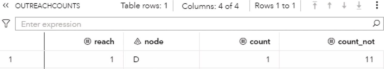
Figure 2.72 Counts for the reach network assigned to node D.
The network projection algorithm can also be seen as a process to reduce multiple partition graphs to a single partition graph. If a network is projected based on a subset of nodes U through another subset of nodes V, the unipartite network produced by this projection will contain only the nodes from the subset U. The links connecting the nodes in the projected network, the one based on the subset of nodes U, are created if these nodes share a common neighbor in the bipartite network, or they are connected to the same nodes in the subset V. The network projection algorithm assumes that the graph that is induced by the union of the two subsets of nodes U ∪ V in the original network is bipartite. Therefore, any possible existing link between the nodes in U or any possible links between the nodes in V, are suppressed.
In proc network, the PROJECTION statement invokes the algorithm to compute the network projection. The algorithm computes the network projection based on nodes specified in the nodes input table. The nodes dataset is defined in proc network by the option NODES =. The nodes dataset contains the subsets of nodes for each partition by specifying the nodes identifiers and the partition flag. In the PROJECTION statement, the option PARTITION = is used to define the partition of each node. The value assigned to that option must be 0, 1, or missing. In order to create a network projection on the nodes set U through the nodes set V, in the nodes dataset the partition flag must be 1 to all nodes from the set U and 0 to all nodes from the set V. Nodes with missing values for the partition flag in the nodes dataset will be ignored, as well as the nodes from the original bipartite network that are not specified in the dataset.
The strength of the connections between the nodes in the projected network can be determined by the number of neighbors they have in common in the bipartite network. Proc network uses different similarity measures to quantify the link weights in the projected network. The current similarity measures are Adamic‐Adar, common neighbors, cosine, and Jaccard.
Network projection can be computed in both undirected and directed graphs. When the graph is based on undirected links, the evaluation of neighbors is straightforward. If nodes a and b from set U are connected to node i from subset V, then nodes a and b will be connected in the projected network. However, if the graph is based on directed links, there are different methods to manage the direction of the links and the concept of neighborhood.
The final results for the network projection algorithm in proc network are reported in the output tables defined by the options OUTPROJECTIONLINKS =, OUTPROJECTIONNODES =, and OUTNEIGHBORSLIST =.
The OUTPROJECTIONLINKS = option defines the output data table containing the links of the projected graph. Additionally, this table can also report the similarity measures computed between the pairs of nodes that are represented by a link in the projected graph. These similarity measures quantify how the pairs of nodes in the subset with partition flag 1 are connected through the nodes in the subset with partition flag 0. This output table contains the following variables:
- from: the from node label of the link.
- to: the to node label of the link.
- adamicAdar: the Adamic‐Adar similarity score between the from and to nodes.
- commonNeighbors: the common neighbors similarity score between the from and to nodes.
- cosine: the cosine similarity score between the from and to nodes.
- jaccard: the Jaccard similarity score between the from and to nodes.
The OUTPROJECTIONNODES = option defines the output table containing the nodes of the projected graph. This output contains the following column:
- node: the node label.
The OUTNEIGHBORSLIST = option defines the output table containing the list of neighbors that are common to each pair of nodes that are joined by a link in the projected graph. Each link listed in the output table defined by the option OUTPROJECTIONLINKS = creates one or multiple records in that neighbor list table. Each neighbor that is common to both from and to in the links table creates a record neighbor list table. This output contains the following columns:
- from: the from node label.
- to: the to node label.
- neighbor_id: the sequential index of the neighbor.
- neighbor: the node label of the common neighbor of the from and to nodes.
The network projection algorithm in proc network contains some additional options to determine what is to be considered when computing the projected network from a bipartite graph.
The option ADAMICADAR = specifies whether to calculate the Adamic‐Adar node similarity measure when quantifying the number of neighbors a pair of nodes have in common. The values for this option are TRUE or FALSE. If true, this node similarity measure is reported in the output table specified by the OUTPROJECTIONLINKS = option. If false, proc network does not calculate Adamic‐Adar node similarity. The default value is false.
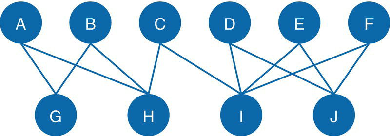
Figure 2.73 Input bipartite graph.
The option COMMONNEIGHBORS = specifies whether to calculate common neighbors node similarity when quantifying the number of neighbors nodes have in common. The options are TRUE or FALSE. If true, proc network calculates the common neighbors node similarity and saves the results in the output table specified by the option OUTPROJECTIONLINKS =. If false, proc network does not calculate common neighbors node similarity. The default value is false.
The option COSINE = specifies whether to calculate cosine node similarity to quantify the common neighbors for the pairs of nodes. The options are TRUE or FALSE. If true, proc network calculates the cosine node similarity and reports the results in the output table specified by the option OUTPROJECTIONLINKS =. If false, proc network does not calculate cosine node similarity, and the default value is false.
Network projection can be computed based on both undirected and directed graphs. On directed graphs, due to the direction of the links and the possible paths of connections throughout the network, different methods may be used to handle the existing relations. The option DIRECTEDMETHOD = specifies the method to be used to compute the network projection when the graph is based on directed links. This option is used only for directed graphs when the option DIRECTION = is specified as DIRECTED. For directed graphs, proc network provides three different methods to handle the directed links. The method CONVERGING considers only the out‐neighbors of nodes in U, which means only the nodes in V that are connected by outgoing links. The method DIVERGING considers only in‐neighbors of nodes in U, which means only nodes in V that are connected by ingoing links. Finally, the method TRANSITIVE considers only paths of length two, which means paths that start at some node in U, traverse through some node in U, and end at some node in U. The default method used in proc network is CONVERGING.
The option JACCARD = specifies whether to calculate the Jaccard node similarity. The possible values are TRUE or FALSE. If true, proc network calculates the Jaccard node similarity and reports the result in the output table specified in the OUTPROJECTIONLINKS = option. if false, node similarity is not calculated, and the default value is false.
The option PARTITION = specifies the name of the variable for the partition flag. The partition variable is defined in the input nodes dataset. The value can be 1 or 0 (or missing). All nodes with the partition variable equal to 1 define the set of nodes that the input graph will be projected on. The links in the projected graph are created based on the nodes that are connected through common neighbors among the set of nodes that have the partition flag of 0. Nodes with the partition flag missing are excluded from the calculation.
Let's see some examples of network projection for both directed and undirected graphs.
2.7.1 Finding the Network Projection
Figure 2.73 shows a bipartite graph containing 10 nodes and 12 links. Nodes A, B, C, D, E, and F do not connect to each other. They represent one partition of the bipartite graph. Similarly, nodes G, H, I, and J do not connect to each other and therefore represent another partition in this bipartite graph. Nodes from one partition (A,B,C,D,E,F) do connect to nodes to the other partition (G,H,I,J).
The following code describes how to create the links dataset. For the network projection, the nodes partitions must also be provided. The nodes dataset with the partition flag is also created. The projected network is based on the subset of nodes A, B, C, D, E, and F. This subset of nodes is set in the nodes dataset with the partition id 1. The nodes projection will be through the common neighbors in the subset of nodes G, H, I, and J. This subset is flagged with partition id 0.
data mycas.links;input from $ to $ @@;datalines;A G A H B G B H C H C I D I D J E I E J F I F J;run;data mycas.partitionnodes;input node $ partitionid @@;datalines;A 1 B 1 C 1 D 1 E 1 F 1 G 0 H 0 I 0 J 0;run;
Once the input links and nodes are defined, proc network can be invoked to compute the network projection on this bipartite input graph. The following code describes how to do that. For this particular execution, all methods to compute the nodes similarities are used, Adamic‐Adar, common neighbors, Cosine, and Jaccard.
proc networkdirection = undirectedlinks = mycas.linksnodes = mycas.partitionnodes;linksvarfrom = fromto = to;projectionpartition = partitionidoutprojectionlinks = mycas.outprojectionlinksoutprojectionnodes = mycas.outprojectionnodesoutneighborslist = mycas.outneighborslistadamicadar = truecommonneighbors = truecosine = truejaccard = true;run;
Figure 2.74 shows the summary output for the network projection algorithm. It shows the size of the network, 10 nodes and 12 links, the direction of the graph, the algorithm used, the time to process, and the final output tables.
The OUTPROJECTIONNODES table presented in Figure 2.75 shows all nodes projected in the network projection. These nodes belong to one partition and are projected based on their common neighbors within the other partition in the bipartite input graph.
The OUTPROJECTIONLINKS table presented in Figure 2.76 shows the links connecting the projected nodes. The nodes similarity scores for all four methods are reported in this output table. Notice the common neighbors measure. It shows how many common neighbors a particular link has. For example, nodes A and B are connected in the projected network because they have 2 common neighbors, nodes G and H in the other partition (A↔G/A↔H and B↔G/B↔H).
The OUTNEIGHBORSLIST table presented in Figure 2.77 shows the common neighbors between the projected nodes based on each link. For example, the link between nodes A and B are created based on the common neighbors G and H (lines 1 and 2 in the output table).
Figure 2.78 shows the final projected network considering only the projected nodes and their links based on the common neighbors.
Let's see how the network projection works on a directed graph, and also change the set of nodes to be projected. Based on the links input data, let's invert the directions of some links to evaluate the final results of the network projection.
The links G→B, H→B and I→E had their original directions inverted (instead of B−G, B−H, and E−I). The subset of nodes to be projected now considers only the nodes A, B, E, and F (nodes C and D were suppressed). The following code describes these changes.
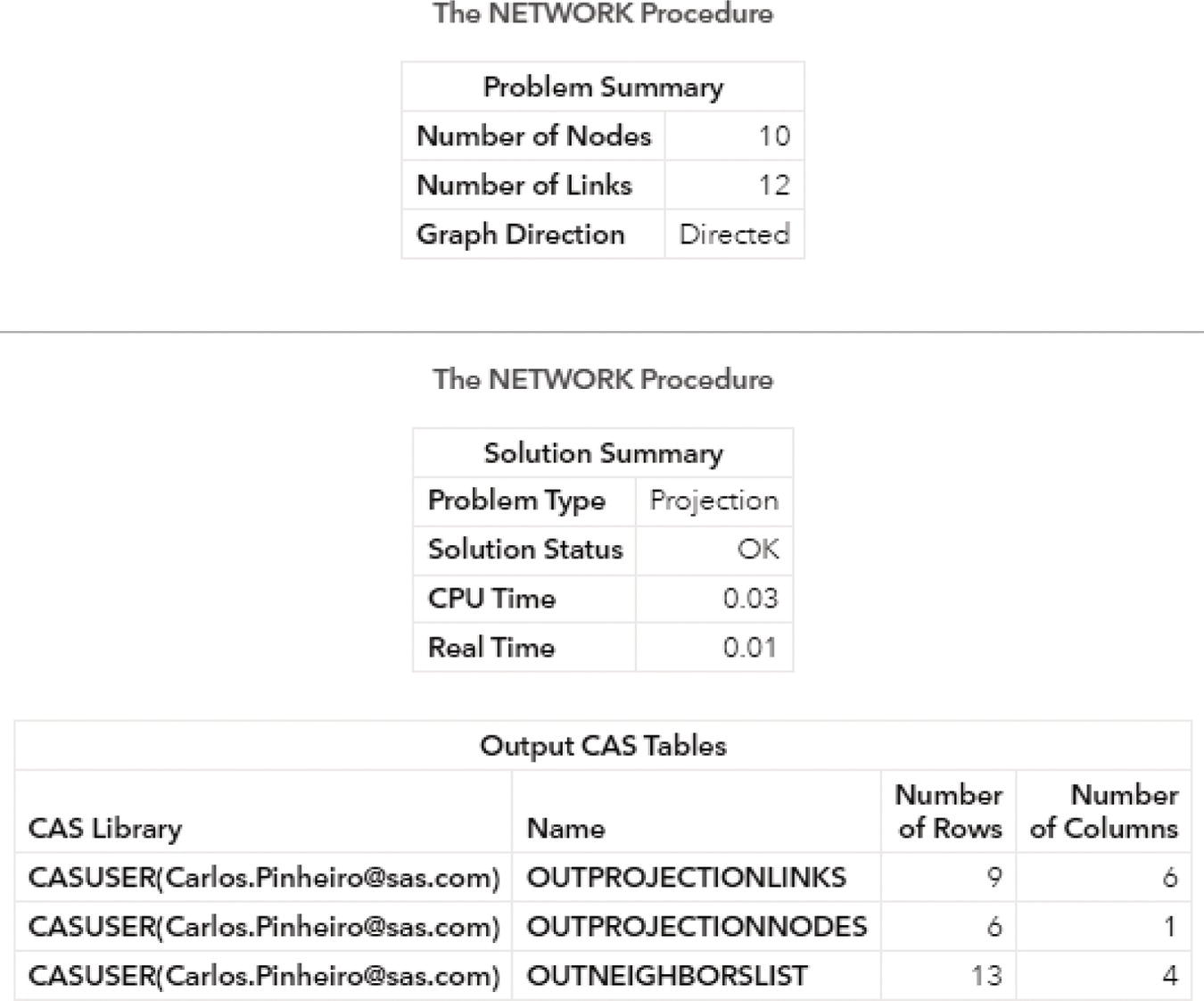
Figure 2.74 Output results by proc network running the network projection algorithm on an undirected graph.
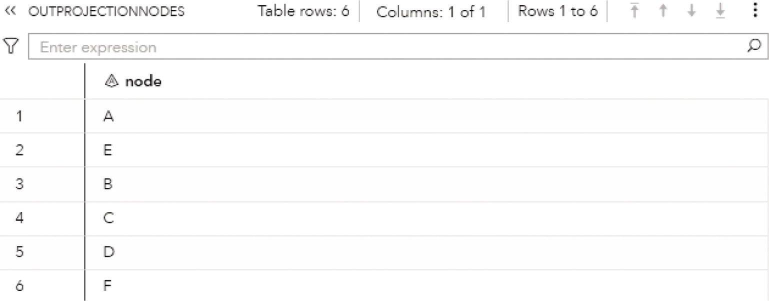
Figure 2.75 Output nodes for the projected network.
data mycas.links;input from $ to $ @@;datalines;A G A H G B H B C H C I D I D J I E E J F I F J;run;data mycas.partitionnodes;input node $ partitionid @@;datalines;A 1 B 1 E 1 F 1 G 0 H 0 I 0 J 0;run;
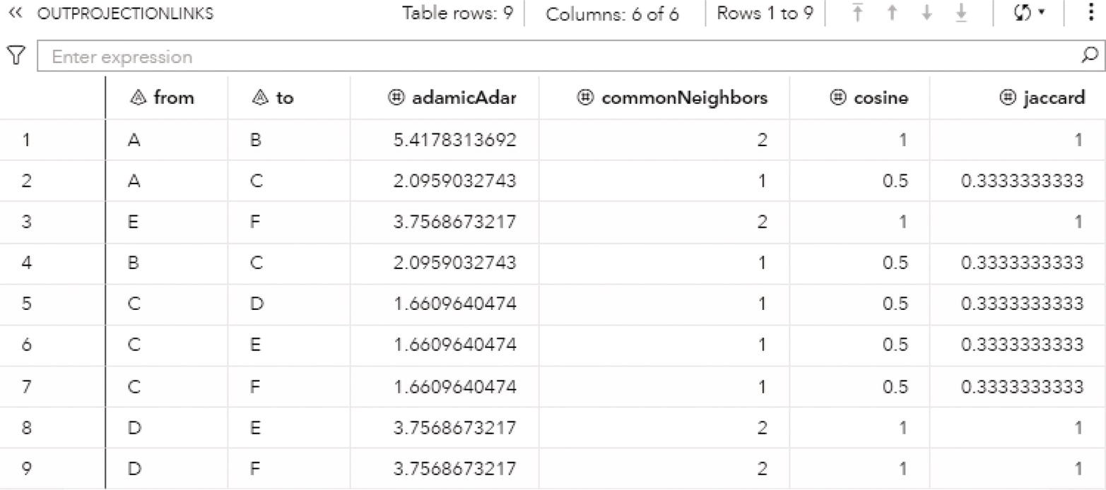
Figure 2.76 Output links for the projected network.
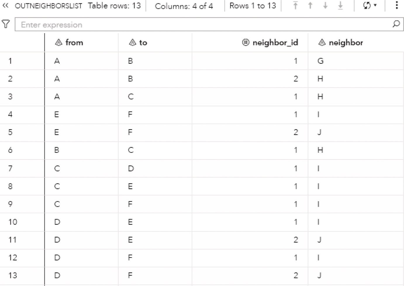
Figure 2.77 Output common neighbors for the projected network.
The new bipartite input graph is presented in Figure 2.79. Nodes C and D, and their respective links are faded out.
One single but important change is made in the code to invoke the network projection algorithm. The direction now is set to directed, and the common neighbors node similarity is calculated. The following code shows these changes.
proc networkdirection = directed...projectionpartition = partitioneddirectedmethod = converging...commonneighbors = true;run;
The OUTPROJECTIONNODES table presented in Figure 2.80 shows only the four nodes projected in partition 1, nodes A, B, E, and F.
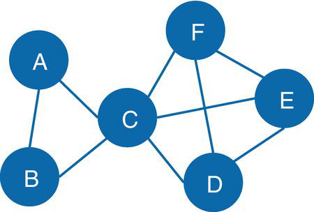
Figure 2.78 Projected network.
The OUTPROJECTIONLINKS table presented in Figure 2.81 shows the single link connecting the projected nodes E and F. They have one single common node (node J in partition 0).
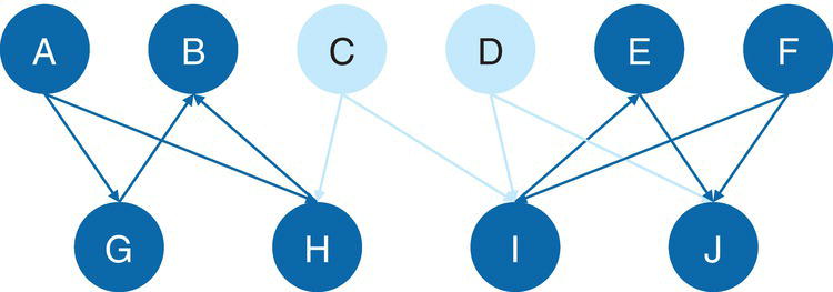
Figure 2.79 Input bipartite graph.
The default method for directed graphs is converging, which considers only the outgoing links from the projected nodes to the common neighbors. Notice that node A points to node G, but node G points to node B. Then, node G is not a common neighbor between nodes A and B based on a directed graph. The same happens for nodes E and F with the former common neighbor node I. Now, node I points to node E and node F points to node I. Node I is no longer a common neighbor between nodes E and F in that configuration. The only projection that remains valid is between nodes E and F through node J. Nodes E and F point to node J, and then, node J is still a common neighbor between those two projected nodes.
The OUTNEIGHBORSLIST table presented in Figure 2.82 shows the only common neighbor (node J) between the projected nodes E and F.
Figure 2.83 shows the final projected network considering the projected nodes and their links based on the common neighbors.
This project network based on the directed graph has only one pair of nodes with a single link between them, as opposed to the previous projected network on the undirected graph with six nodes and nine links.
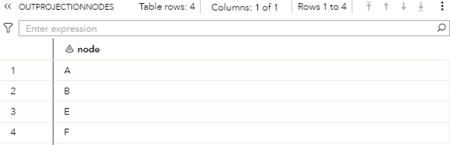
Figure 2.80 Output nodes for the projected network.
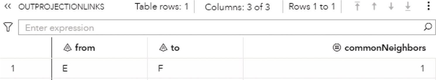
Figure 2.81 Output links for the projected network.
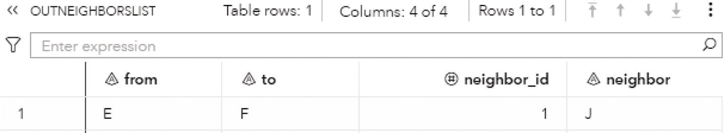
Figure 2.82 Output common neighbors for the projected network.

Figure 2.83 Projected network.
2.8 Node Similarity
Network analysis is a fundamental tool to evaluate relationships and uncover hidden information about entities. Particularly in social networks, the analysis of the nodes' relationships can reveal useful insights about the nodes' characteristics or attributes. That means in network analysis, analyzing the links can disclosure relevant information about the nodes. In other words, analyzing the relations between nodes can describe the roles or functions of the nodes. One important concept about the nodes based on their links is the node similarity. Node similarity has many applications in business, science, and social studies, among others. Companies can use node similarity to make better recommendations upon customers' relationships with products and services, or even between them. Government agencies can use node similarity to predict connections between similar nodes and possibly identify terrorists' relationships. Functions and roles within networks or subnetworks can be better explained by nodes similarities. In medical research, node similarity can be used to study diseases and treatments. In the social domain, node similarity can be used to identify unusual behavior or behavioral changes within communities or throughout different groups. Most of the techniques in node similarity consider the neighborhood of the nodes to identify or quantify a measure of similarity. For example, nodes with the same neighbors would be considered similar. These nodes would have similar links to other nodes. The labels or roles within the network are usually propagated through the links, and then those nodes would be similar because they would have similar labels, roles, or functions with the network.
In graph theory, node similarity measures the similarity of nodes neighborhoods. There are several methods to measure this similarity between nodes. Different algorithms evaluate and compute the similarity between two nodes in particular ways. The most common method is based on the immediate neighborhood of two nodes. That means two nodes are similar if they have the same neighbors. Other methods are based on the structural role proximity of the network around two particular nodes. Instead of searching for the same neighbors between two nodes, these methods search for the similar network structure assigned to these two nodes. The network structure is commonly represented by the first and second order proximity (higher orders of proximity can also be accounted for). Based on these methods, two nodes located far away from each other within the network can still be similar if they have the same structural role proximity. For example, both nodes are center of a star structure, connecting the same number of nodes in first and second order proximity. Even though they are far away apart, they are similar in roles within the network, and then they are considered similar. These methods open up a wide range of possibilities when searching for similar nodes in multiple industries or disciplines in science. For instance, consider a network representing global trading between countries. Two countries may be similar if they trade with the same countries (share the same neighbors). However, two countries far away from each other with no shared neighbors, can also be similar if they trade with other countries and have the same structural role proximity (same number of first and second order proximity creating a similar network structure).
Figure 2.84 shows two similar nodes A and B based on their same set of neighbors.
Figure 2.85 shows two similar nodes A and T based on their same structure role proximity, even though they might be far away from each other in the network.
In proc network, the NODESIMILARITY statement invokes the algorithm to quantify the node similarity within the network. There are six algorithms to quantify the node similarity. Four of them use the concept of same neighbors to evaluate how similar two nodes are. Two others use the concept of the structural role proximity to quantify how similar two nodes are. The four algorithms to quantify the node similarity based on the nodes' neighbors are Common Neighbors similarity, Jaccard similarity, Cosine similarity, and Adamic‐Adar similarity.
A straightforward method to quantify node similarity within a network is to assess the number of neighbors that two nodes have in common. In other words, two nodes are similar based on a proportion of the size of their neighborhoods that overlapped.
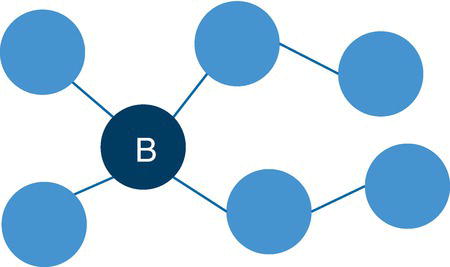
Figure 2.84 Similar nodes based on their neighborhood.
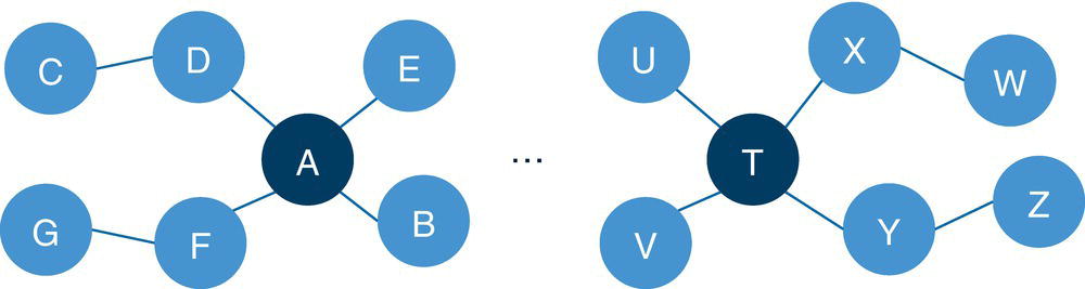
Figure 2.85 Similar nodes based on their structural role proximity.
For example, let's assume an undirected graph ![]() that represents the set of neighbors of node i, excluding the node i itself. That means unique nodes that are connected by links to node i. In a directed graph, there are two sets of neighbors of node i, considering the outgoing links and the incoming links incident to node i. The first set
that represents the set of neighbors of node i, excluding the node i itself. That means unique nodes that are connected by links to node i. In a directed graph, there are two sets of neighbors of node i, considering the outgoing links and the incoming links incident to node i. The first set ![]() represents the set of out‐neighbors of node i, excluding node i itself. In that case, it considers all unique nodes that are connected to node i by outgoing links. The second set
represents the set of out‐neighbors of node i, excluding node i itself. In that case, it considers all unique nodes that are connected to node i by outgoing links. The second set ![]() represents the set of in‐neighbors, excluding node i itself. That set considers all unique nodes that are connected to node i by incoming links. The common neighbors measure can be calculated for both undirected and directed graphs. For undirected graphs, the measure to quantify the similarity between nodes i and j based on their neighborhood is defined by the following equation:
represents the set of in‐neighbors, excluding node i itself. That set considers all unique nodes that are connected to node i by incoming links. The common neighbors measure can be calculated for both undirected and directed graphs. For undirected graphs, the measure to quantify the similarity between nodes i and j based on their neighborhood is defined by the following equation:
For directed graphs, as the similarity considers the outgoing and incoming links to nodes i and j differently, the measure is calculated by the following equation:
The measure based on common neighbors favors nodes with multiple connections. Then, nodes with high degree centrality are most likely to have large similarity scores, even when they have a small number of common neighbors connected to them.
The Jaccard similarity aims to correct the bias created by the high degree centrality. This measure is similar to the common neighbors similarity, but it divides the common neighbors measure by the number of nodes within the two nodes i and j neighbors sets, which means the union of the two sets of neighborhoods. For undirected graphs, the Jaccard similarity measure is defined by the following equation:
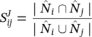
For directed graphs, the Jaccard similarity considers the out‐neighbors and the in‐neighbors sets created by the outgoing and incoming links incident to nodes i and j. The measure is calculated by the following equation:
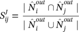
If nodes i and j are the same, then the Jaccard similarity measure equals to 1. If the nodes i and j are different but the union of their neighborhoods is empty, the Jaccard similarity measure equals to 0.
The Cosine similarity is another method used to reduce the bias created by the high degree centrality on the common neighbors. The Cosine similarity uses the cosine of the angle between the two vectors that represent the sets of neighbors for nodes i and j. For undirected graphs, the Cosine similarity measure is defined by the following equation:
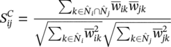
In the Cosine similarity measure, ![]() and
and ![]() represent the parallel link weights between the nodes i and k, and j and k, respectively. This parallel link weight can be formulated by the following equation:
represent the parallel link weights between the nodes i and k, and j and k, respectively. This parallel link weight can be formulated by the following equation:
where ![]() is the sum of the parallel link weights between the nodes i and j.
is the sum of the parallel link weights between the nodes i and j.
For directed graphs, the Cosine similarity considers the out‐neighbors and in‐neighbors separately. The measure is calculated by the following equation:
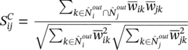
The parallel link weights in directed graphs consider the outgoing and incoming links between the nodes. The sum of parallel link weights in directed graphs is defined by the following equation:

If a graph is defined with no link weights, w ij is set by convention to 1. If nodes i and j are the same, then the Cosine similarity measure equals to 1. If the nodes i and j are different but either of the two neighborhoods sets is empty, the Cosine similarity equals to 0.
The Adamic‐Adar similarity measure is a third way to correct the bias created by the high degree centrality in the common neighbors similarity measure. The Adamic‐Adar similarity aims to discount the contribution of common neighbors that have high degree centrality. The Adamic‐Adar is quite different than the similarity measures Jaccard and Cosine. Both Jaccard and Cosine similarities are relative measures assigning a score to a pair of nodes i and j. This score is relative to the proportion of the neighborhoods sets of i and j that overlap. Adamic‐Adar similarity on the other hand is an absolute measure. It assigns to each common neighbor of nodes i and j an inverse log weight. By doing this, Adamic‐Adar similarity measure discounts connections that are very weak. For example, two nodes i and j have mutual connections to a particular node k, which, for example, is a hub in the network with a very high degree centrality. The Adamic‐Adar similarity measure will discount the importance of this common neighbor for nodes i and j because of its high degree centrality. For undirected graphs, the Adamic‐Adar similarity measure is defined by the following equation:

For directed graphs, the Adamic‐Adar similarity considers the out‐neighbors for each pair of nodes and the in‐neighbors for the common neighbor nodes. The measure is calculated by the following equation:
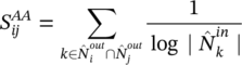
The previous four similarity measures consider the common neighbors that a pair of nodes have. Another method to compare nodes within the network is by evaluating their structural roles in the graph, particularly how they are connected to other nodes by first and second orders of proximity. This method commonly embeds the nodes within a graph by creating a multidimensional vector space that preserves the original network structure. These multidimensional vectors aim to capture the first and second order proximity between nodes. The proximity between nodes corresponds to the proximity between the vector space embeddings. The first order proximity is the local pairwise proximity between two connected nodes. It can be represented w ij , which is the sum of the link weights between nodes i and j. The first order proximity captures the direct neighbor relationships between nodes. The second order proximity captures the two‐step relations between each pair of nodes. For each pair of nodes, the second order proximity is determined by the number of common neighbors shared by the two nodes, which can be measured by the two‐step transition probability from node i to node j equivalently. The second order proximity between a pair of nodes i and i is the similarity between their neighborhood structures. Ultimately, the second order proximity, or even higher order, captures the similarity of indirectly connected nodes with similar structural context.
The first order proximity of node i to all other nodes in the graph can be represented by the embedded vector p i = (w i1, …, w i ∣ n∣). The second order proximity between nodes i and j is determined by the similarity between their embedded vectors p i and p j . The second‐order proximity assumes that the nodes that share many connections to other nodes are similar to each other in their structural roles. This method calculates a multidimensional vector u i for each node i by minimizing a corresponding objective function. The objective function for the first order proximity is defined by the following equation:
where from(ij) is the from (source) node of the link ij, to(ij) is the to (sink) node of link ij, and p 1 is the joint probability of a link between nodes i and j. The join probability between two nodes can be calculated by using the following formula:
For the second order proximity, the multidimensional vector u i and the multidimensional context embeddings v i are calculated by minimizing the objective function defined by the following equation:
Where the multidimensional context p 2(j ∣ i) can be calculated by the following formula:

The optimization method used to minimize the objective function is based on the stochastic gradient descent algorithm. This algorithm uses a random sampling of the links from the input link dataset defined to describe the graph. The stochastic gradient descent algorithm runs multiple iterations updating the embedding vector space. Once the objective function stops improving, the algorithm converges, and the optimization process terminates before running all samples specified. The tolerance for this convergency can also be specified, defining the rate of changes in the embedding vectors and how the objective functions are minimized throughout the iterations. Optimizing the embedding vectors without any change in the formulation can be expensive. A more efficient way of deriving the embedding vectors is by using negative sampling. The negative sampling is in fact a different objective function and is used to approximate the loss. The embedding vector algorithm uses a random distribution over all nodes in the input graph. Instead of normalizing with respect to all nodes, the negative samples just normalize against k random nodes. In this way, to compute the loss function, only k negative samples proportional to the degree can be used.
The embedding vector space is computed for each node within the graph. Then, the vector similarity between each pair of nodes i and j is calculated as a function of the angle between the embedded vectors for i and j. The angle between the embedded vectors between a pair of nodes is calculated by using the following equation:
where ![]() is the angle between u i and u j .
is the angle between u i and u j .
Computing node similarity, particularly for large graphs, can be expensive. By default, proc network calculates the node similarity for every pair of nodes within the network. To diminish the computation cost for this calculation, a subset of nodes can be defined when calculating the node similarity. Two different subsets of nodes can be defined to drive the node similarity calculation. The first set defines the source (origin) nodes. The second set defines the sink (destination) nodes. For undirected graphs, source and sink nodes do not represent the beginning nor the end of the links. For directed graphs, the source nodes do represent the beginning of the links, its origin, and the sink nodes represent the end of the links, its destination. The NODESSUBSET = option in proc network define the subset of nodes to be used when computing the node similarity, considering a subset of source nodes and distinctly a subset of sink nodes. Finally, a specific source node and/or sink node can be defined. By doing this, the node similarity will be computed only for this specific pair of nodes. The options SOURCE = and SINK = define a single pair of nodes to be used when computing the node similarity.
The final results for the node similarity algorithm in proc network are reported in the output tables defined by the options OUTSIMILARITY =, OUTNODES =, and OUTCONVERGENCE =. These output tables contain several columns, providing detailed information about the outcomes of the node similarity algorithm.
The OUTSIMILARITY = option defines the output table containing the similarity score for each pair of nodes within the network, or specified in the options NODESSUBSET =, SOURCE =, or SINK =. This output table can be large depending on the size of the network and the number of pairs of nodes to have the node similarity calculated. Depending on the size of the network, the time to produce this output table can be higher than to compute the node similarity. To minimize the cost to produce this output table when computing the node similarity for large networks, proc network allows a filter for sparse similarity. The option SPARSE = defines when to output the similarity score for sparse nodes, or for nodes with no common neighbors, or when the pair of nodes has the same source and sink node. If TRUE, these pairs of nodes are excluded from the output. If FALSE, these pairs of nodes are included to the output table. Proc network can also define when to compute the embed vector for the nodes by specifying the option VECTOR =. When calculating the embed vectors, it is not possible to exclude from the output the spare pairs of nodes. This output contains the following columns:
- source: the label of the source node of this pair.
- sink: the label of the sink node of this pair.
- link: a flag indicating if this pair of nodes exists in the links dataset. If the pair of nodes exists as a link in the input dataset, the flag is 1, or 0 otherwise.
- order: the ranking of each pair of nodes ordered by decreasing similarity score. The score is reported when the options TOPK = or BOTTOMK = are specified.
- jaccard: the Jaccard similarity score when the JACCARD = option is specified.
- commonNeighbors: the common neighbors similarity score when the COMMONNEIGHBORS = is specified.
- cosine: the cosine similarity score when the COSINE = option is specified.
- adamicAdar: the Adamic‐Adar similarity score when the ADAMICADAR = option is specified.
- vector: the vector similarity score when the VECTOR = option is specified.
The OUTNODES = option defines the output table containing the vector representations for each node within the input graph. This output table is produced when the option VECTOR = is TRUE. The columns are reported based on the specification of other options. The vector embedding columns are defined as vec_1 through vec_d, where d is the number of dimensions computed in the embed vector specified in the option NDIMENSIONS =. The embed vector can use the first and the second order of proximity. If the option PROXIMITYORDER = is specified as SECOND, the output table also contains the context embedding columns, defined as ctx_1 through ctx_d, where d is the number of dimensions computed in the embed vector.
The OUTCONVERGENCE = option defines the output table containing the convergence curves for the vector embeddings for all nodes during the training process. The convergence value is periodically reported to the output table during the training process. Similar to the similarity scores, this output table can be quite large depending on the size of the network. To reduce the cost of reporting this outcome, the algorithm reports only at certain sample intervals. This output contains the following columns:
- worker: the identifier for the machine that reports the convergence value.
- sample: the number of samples that have been completed when the convergence value is reported.
- convergence: the reported convergence value.
Proc network produces six similarity measures. The different measures can be computed in parallel, in the same execution of proc network. Each similarity measure has an option to specify and invoke the correct algorithm to compute the different scores.
The option COMMONNEIGHBORS = specifies whether to calculate common neighbors node similarity. If the option is TRUE, proc network calculates the common neighbors node similarity and reports the results in the output table that specified in the OUTSIMILARITY = option. If the option is FALSE, the common neighbors node similarity is not calculated.
The option JACCARD = specifies whether to calculate the Jaccard node similarity. If the option is TRUE, proc network calculates the Jaccard node similarity and reports the results in the output table specified in the OUTSIMILARITY = option. If the option is FALSE, the Jaccard node similarity is not calculated.
The option COSINE = specifies whether to calculate the cosine node similarity. If the option is TRUE, proc network calculates the cosine node similarity and reports the results in the output table specified in the OUTSIMILARITY = option. If the option is FALSE, the cosine node similarity is not calculated.
The option ADAMICADAR = specifies whether to calculate the Adamic‐Adar node similarity. If the option is TRUE, proc network calculates the Adamic‐Adar node similarity and reports the results in the output table specified in the OUTSIMILARITY = option. If the option is FALSE, the Adamic‐Adar node similarity is not calculated.
Those are the four methods to compute the node similarity based on the neighborhood of each node. The other two methods are based on the structural roles' proximity within the network.
The option VECTOR = specifies whether to calculate vector node similarity. If the option is TRUE, proc network calculates the vector node similarity and reports the results in the output table specified in the OUTSIMILARITY = option. If the option is FALSE, the vector node similarity is not calculated. When calculating the vector node similarity (VECTOR = TRUE), other options are available to define the type of the calculation.
The option PROXIMITYORDER = specifies the type of the proximity to use in the vector algorithm. If the option is FIRST, proc network uses the first‐order proximity when computing the embed vector. If the option is SECOND, proc network uses the second‐order proximity when computing the embed vector.
The option EMBED = specifies whether to calculate vector embeddings. If the option is TRUE, proc network calculates the vector embeddings and reports the results in the output table specified in the OUTNODES = option. If the option is FALSE, the vector embeddings is not calculated.
The option EMBEDDINGS = specifies the variables to be used as precalculated vector embeddings. Multiple columns can be specified in the embeddings. The values assigned to the columns used in the embeddings must be numeric (no missing) and must exist for each node in the input graph. The variables used in the embeddings must be specified in the input dataset defined by the option NODES =. In order to compute the embeddings using a list of variables, the options VECTOR = and EMBED = must be TRUE.
The option NDIMENSIONS = specifies the number of dimensions for node‐embedding vectors.
The option NSAMPLES = specifies the number of training samples for the vector algorithm. The value assigned to the number of samples by default is 1000 times the number of links in the input graphs.
The option NEGATIVESAMPLEFACTOR = specifies a multiplier for the number of negative training samples per positive training sample for the vector algorithm. The vector algorithm uses the number specified in the option NSMAPLES = as positive samples and that number times the number assigned to the option NEGATIVESAMPLEFACTOR = as negative samples. For example, if NSAMPLES = 1000 and NEGATIVESAMPLEFACTOR = 5, the vector algorithm uses 1000 positive samples and 5,000 negative samples. Recall that the negative sample is smaller and proportional to the degree, instead of a random sample against to all nodes in the input graph. In practice, the k used as a factor for the negative sample is between 5 and 20. The default in proc network is 5. The default number of samples is 1000.
The option CONVERGENCETHRESHOLD = specifies the convergence threshold when computing the vector similarity. If the convergence value drops below this threshold before proc network completes the number of samples specified in the option NSAMPLES =, the vector embeddings training terminates early.
The option ORDERBY = specifies the similarity measure to use when ranking the pairs of nodes reported in the output table specified in the option OUTSIMILARITY =. The options are the different similarity measures computed by proc network, COMMONNEIGHBORS, JACCARD, COSINE, ADAMICADAR, and VECTOR. The ORDERBY = option is used in conjunction with the options TOPK = and BOTTOMK =.
The option TOPK = specifies the maximum number of highest‐ranked similarity pairs to be reported in the output table specified in the option OUTSIMILARITY =. If multiple similarity measures are computed, the option ORDERBY = must be used to define which similarity measure is used to rank the pairs in the output table.
Similarly, the option BOTTOMK = specifies the maximum number of lowest‐ranked similarity pairs to be reported in the output table defined by the option OUTSIMILARITY =. Again, when multiple similarity measures are calculated, the option ORDERBY = defines the similarity measure used to rank the pairs in the output table.
The option MAXSCORE = specifies the maximum similarity score to report in the output table specified in the option OUTSIMILARITY =. The similarity score ranges from 0 to 1. This option is supported only for the Jaccard and vector similarity measures. By default, the possible maximum score 1 is used.
The option MINSCORE = specifies the minimum similarity score to report in the output table specified in the option OUTSIMILARITY =. Similarly, this option is supported only for the Jaccard and vector similarity measures. By default, the minimum possible score 0 is used.
Let's see some examples of node similarity for both directed and undirected graphs.
2.8.1 Computing Node Similarity
In order to demonstrate the node similarity algorithm, let's consider a graph similar to the one presented at the beginning of this section, shown in Figure 2.86, with some additional nodes and links. This graph has 18 nodes and 18 links. Initially this graph will be considered an undirected graph, with no link weights.
The following code describes how to create the input links dataset.
data mycas.links;input from $ to $ @@;datalines;A E A B A F A D A H A I D C F GT U T V T X T Y T R T S X W Y ZE V B U;run;
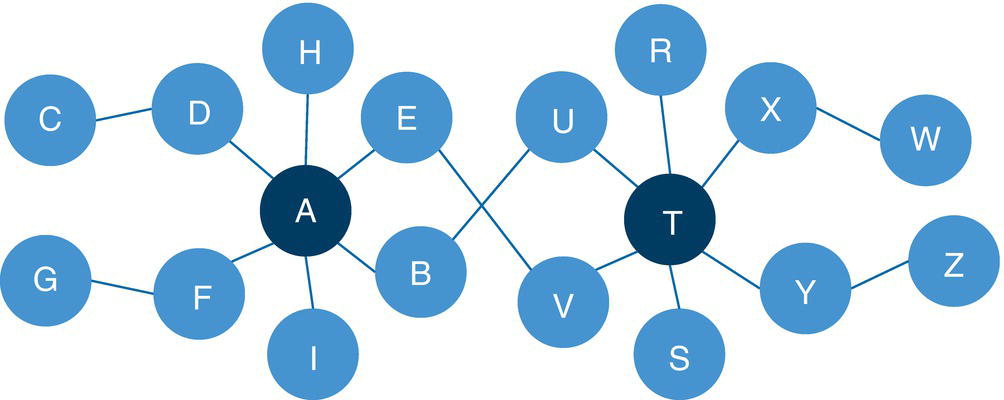
Figure 2.86 Input undirected graph.
Once the input links dataset is defined, we can invoke the node similarity algorithm in proc network. The following code describes the computation of all possible node similarity measures:
proc networkdirection = undirectedlinks = mycas.linksoutnodes = mycas.outnodesvectors;linksvarfrom = fromto = to;nodesimilaritycommonneighbors = truejaccard = truecosine = trueadamicadar = truevector = truendimensions = 100proximityorder = secondoutsimilarity = mycas.outsimilarity;run;
Figure 2.87 shows the summary output for the node similarity algorithm. It shows the size of the network, the direction of the graph and the output tables created.
The OUTNODESVECTORS table presented in Figure 2.88 shows all nodes from the original input graph and the values for each vector dimension. In the proc network code, the option NDIMENSIONS = 100 requests the algorithm to compute a vector with 100 dimensions. Each dimension is represented by a column name vec_x, where x varies from 1 to 100. This vector can be used to warm start the node similarity calculation when the EMBEDDINGS = option is defined.
The OUTSIMILARITY table presented in Figure 2.89 shows the pairs of nodes from the input graph where the node similarity measures were computed. In our case, five measures were calculated, Common Neighbors, Jaccard, Cosine, Adamic‐Ada, and the vector node similarity with second order proximity. This output table also shows whether or not the pair of nodes have a link between them. Notice that this outcome can be extensive, particularly when large networks are used as input for the node similarity algorithm. Also, an auto‐relationship is assumed making the algorithm to compute the node similarity for pairs of nodes where source and sink are the same. For example, the node similarity for E as a source node and E as a sink node is 1. The number of common neighbors in that case is the number of connections this particular node has.
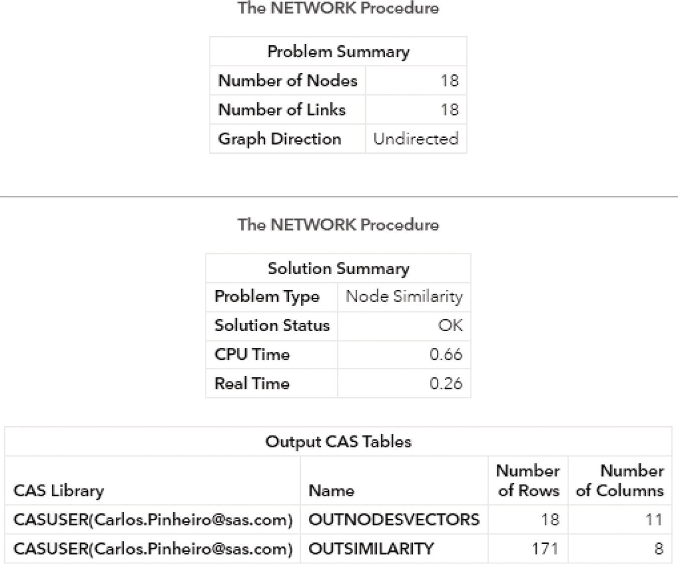
Figure 2.87 Output results by proc network running the node similarity algorithm.
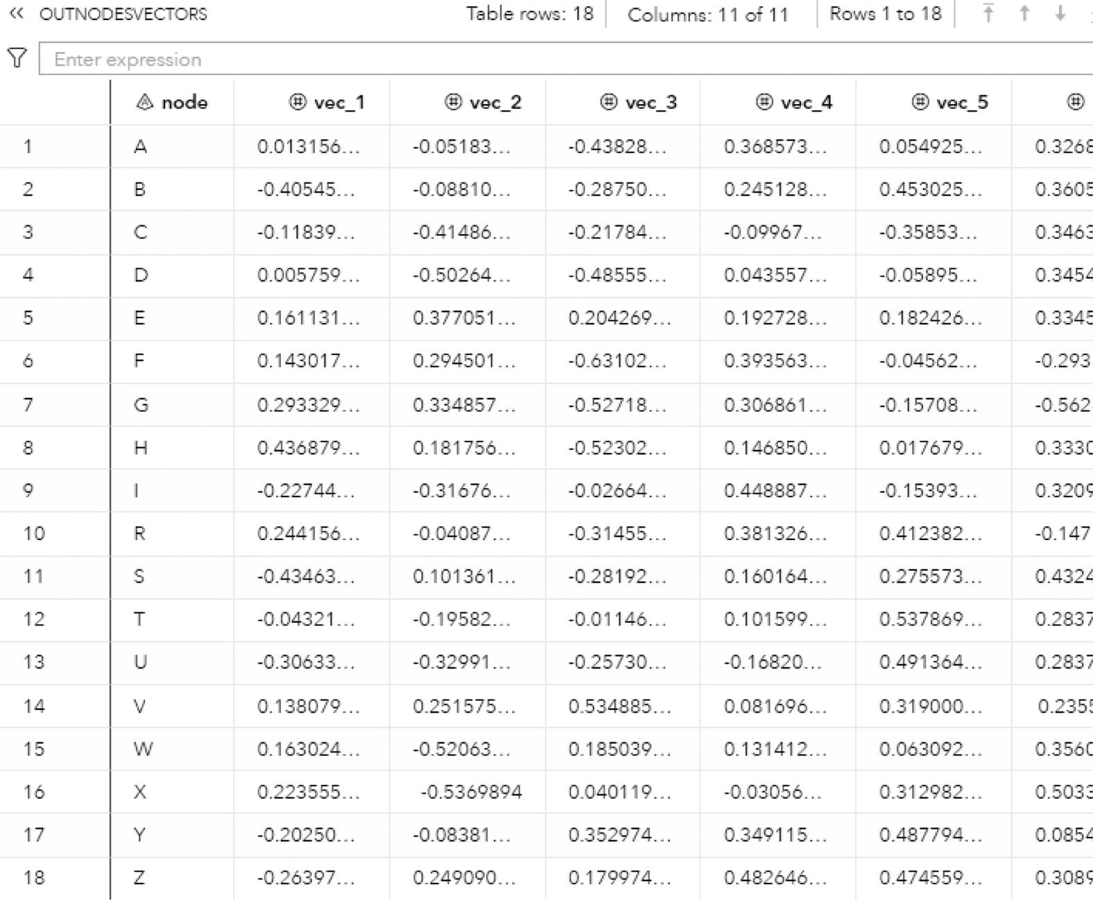
Figure 2.88 Output vectors for the node similarity.
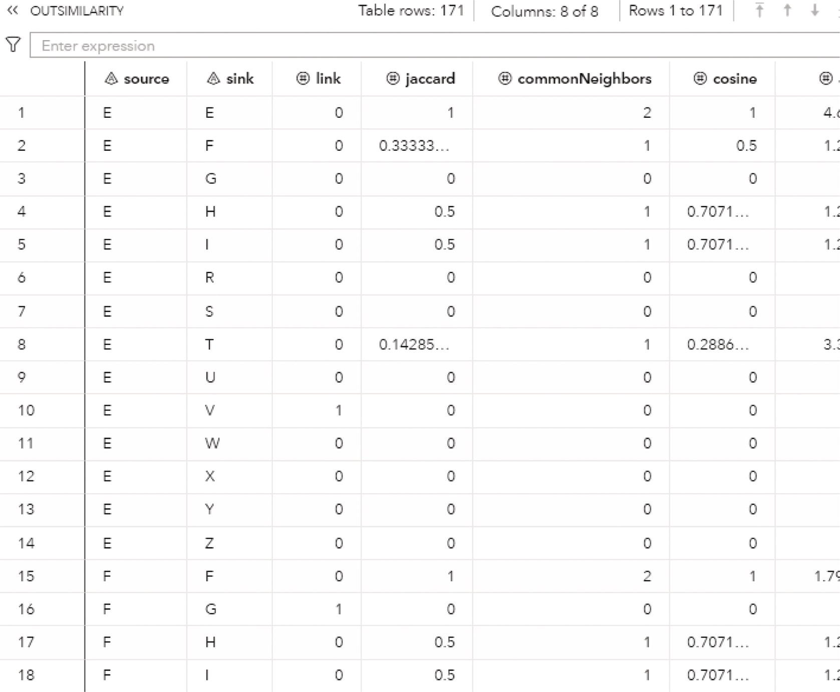
Figure 2.89 Output node similarity measures.
We are not actually interested in the similarity of the same node, or the similarity measure between the node and itself. The following code creates a similar output without the pairs of nodes where source and sink are the same:
data mycas.outsimilarityunique;set mycas.outsimilarity(where=(source ne sink));run;
The OUTSIMILARITYUNIQUE table shows the node similarity measures for the real pair of nodes (not considering the assumed auto‐relationships).
Figure 2.90 shows only the top 2 pairs of nodes based on the Jaccard node similarity.
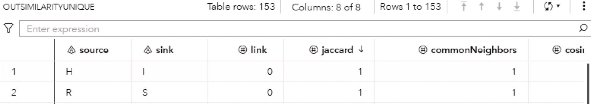
Figure 2.90 Output node similarity for the top Jaccard measure.
Nodes H and I, as well as nodes R and S have the Jaccard node similarity equal 1, the maximum value possible. Node H has only one connection, to node A, and node I has only one connection, also to node A. These nodes are similar because they have the same neighbors, in this case, only one.
We can also compute the node similarity based on a specific pair of source and sink nodes. A minor change in the code invokes proc network to compute the node similarity only between the nodes A and T, as shown in the following excerpt of code:
proc network...nodesimilaritysource = 'A'sink = 'T'...run;
The OUTSIMILARITY table presented in Figure 2.91 shows the node similarity measures for one single pair of nodes, considering node A as the source node and node T as the sink node.
Notice that even though nodes A and T have node connection between them, and no common neighbor, they are sort of similar because of their structural role proximity.
In addition to the SOURCE = and SINK = options to define a single pair of nodes, proc network can use a definition of a subset of nodes to consider a set of nodes as source nodes and a different set as sink nodes. The following code describes how to define a subset of source and sink nodes to be used in proc network to compute the node similarity to a set of pairs of nodes instead of the entire network:
data mycas.nodessim;input node $ source sink @@;datalines;A 1 0 D 1 0 F 1 0T 0 1 X 0 1 Y 0 1;run;
Once the subset of nodes is defined, it must be referenced in proc network. The following code excerpt describes how to do that.
proc networkdirection = undirectedlinks = mycas.linksnodessubset = mycas.nodessim...nodesimilarity...run;
The NODESSIM table defines 3 nodes as sources by using the variable source equals 1 and the variable sink equals 0. Nodes A, D, and F are defined as source nodes. Nodes T, X, and Y are defined as sink nodes by setting the variable source equals 1 and the variable sink equals 0.
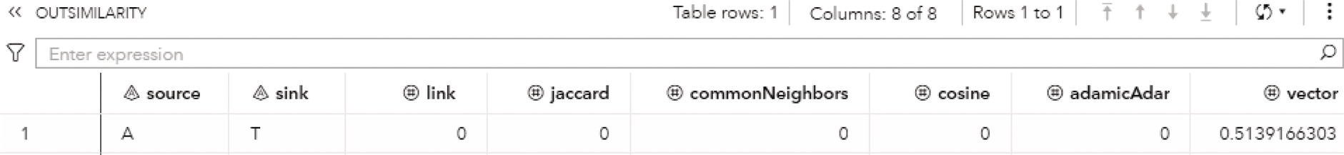
Figure 2.91 Output node similarity measures for the pair of nodes A and T.
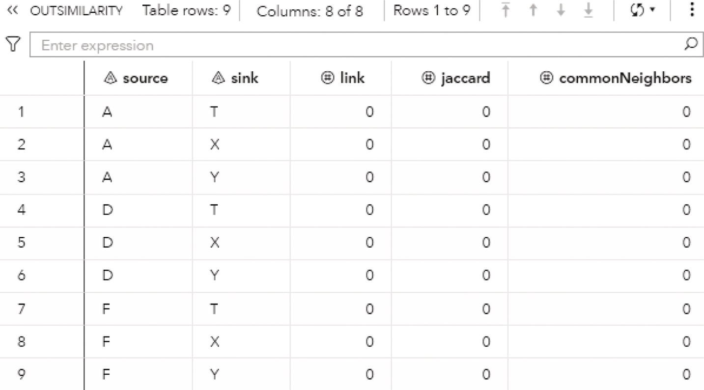
Figure 2.92 Output nodes similarity.
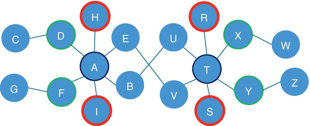
Figure 2.93 Node similarity outcomes.
The OUTSIMILARITY output table presented in Figure 2.92 now shows only the node similarity measures for the pairs of nodes defined in the subset of nodes presented before.
Figure 2.93 shows some pairs of nodes that were considered similar based on some node similarity measures. For example, nodes H and I, as well as nodes R and S have the highest Jaccard similarity measure. Nodes A and T have a high vector similarity measure. Nodes D and F, as well as nodes X and Y have a high common neighbors similarity measure.
Finally, node similarity can also be calculated for directed graphs. The only change needed is the definition of the graph direction in proc network, as shown by the following code excerpt:
proc networkdirection = directed...run;
The directed graph considers the information flow created by the direction of the graphs, which affects the concept of neighbors, and then the calculation of the node similarity. Considering for example exactly the same network, by using the links creation to define the direction of the connections, the node similarity algorithm presents a quite different result. Based on an undirected graph, several pairs of nodes got the maximum node similarity measure, for example, Jaccard equals 1. However, based on a directed graph, considering the same network, only 2 pairs of nodes got a Jaccard measure as 0.16 and all other pairs got 0 as node similarity.
The output table OUTSIMILARITYUNIQUE presented in Figure 2.94 selects all rows from the original OUTSIMILARITY table excluding the observations where the source node equals to the sink node.
Node similarity can be particularly useful to find nodes with common neighbors or nodes with similar structural role proximity. This information can be used to search similar behaviors or connections within large networks. Suppose that an illegal transaction is detected in the transactional system. The entity committing this transaction probably have connections to other entities. By computing the node similarity, similar types of connections or similar relationship behaviors can be found in a large network and highlight possible illegal transactions that were not captured yet by the transaction systems.
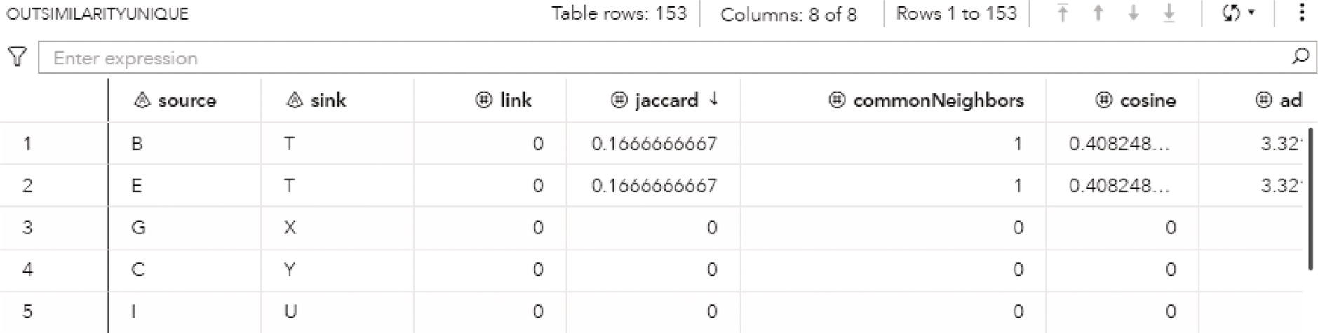
Figure 2.94 Output node similarity measures for a directed graph.
2.9 Pattern Matching
Node similarity is a method to search similar actors or entities within network structures that somehow present comparable or alike connections, common neighbors, or structural roles proximity. Another method to find similarities within networks is to search for whole graph structures. Graph pattern matching has many applications, from plagiarism detection, to biology, social networks, image recognition, intelligence analysis, and fraud investigation, among many others.
Pattern matching or graph matching is the problem of finding a homomorphic or isomorphic subgraph within an input graph. This subgraph is called the patterns in the given input graph, called the target. This problem is also referred to as subgraph a homomorphism or subgraph isomorphism problem. The pattern matching is commonly defined in terms of the subgraph isomorphism, or the search for subgraphs of a given input graph that matches to a query graph. For example, suppose a social network structure composed by friends, where they live, and what soccer team they support. The nodes in this network are then persons, locations, and teams. The links are “is friends of,” “lives in,” and “support.” For example, a node Carlos (person) is connected to a node Cary (location) by a link “lives in” and is connected to a node Fluminense (team) by a link “support.” A common pattern matching search in this social network would be to find friends of Carlos who also support Fluminense and live in the same city. The query graph would be any person node connected to team node Fluminense by the link “support” and connected to the city node Cary by the link “lives in.” The main drawback in pattern matching is that searching for subgraphs isomorphism can be complex and extremely time consuming.
Formally, pattern matching can be defined considering a main graph and a query graph. Subgraph isomorphism given a main graph G and a query graph Q is the problem of finding all subgraphs Q ′ of G that are isomorphic to Q. The subgraph Q ′ must have the same network structure or topology of the subgraph Q. The pattern matching problem considers the attribute of nodes and links in the network structure, like in the example previously described. Nodes may be of multiple types, like person, location, and team, as well as the links, as friends of, lives in, and support. The problem is the process of finding all subgraphs Q ′ of G isomorphic to subgraph Q where all attributes for the nodes and links defined for the subgraphs Q are preserved in the subgraphs Q ′.
In proc network, the PATTERNMATCH statement invokes the algorithm to search for the isomorphic subgraphs of a query graph given an input graph. The query graph is defined by using the options LINKSQUERY = and NODESQUERY =. These options can be used independently to define the query graphs. For example, just the links attributes can be defined as a query graph, just the nodes attributes, or both. The attributes definition for the query graph follows a similar criterion to define attributes for the main input graph. The graphs are created as links and nodes input tables. The main graph is defined by using the options LINKS = and NODES = in proc network. The query graph is defined by using the options LINKSQUERY = and NODESQUERY =. The attributes of the links and nodes in the main graph are defined by using the options LINKSVAR = and NODESVAR in proc network. The attributes of the nodes and links in the query graph are defined by using the options LINKSQUERYVAR = and NODESQUERYVAR.
The final results for the pattern matching algorithms in proc network are reported in the output tables defined by the options OUTMATCHGRAPHLINKS=, OUTMATCHGRAPHNODES=, OUTMATCHLINKS=, OUTMATCHNODES=, OUTQUERYLINKS=, OUTQUERYNODES=, and OUTSUMMARY=. These output tables may contain several columns and vary based on the definition of the query graph and the pattern matching searching, which are defined by the multiple possible parameters in proc network.
The OUTMATCHGRAPHLINKS = option defines the output table containing the links in the induced subgraph of matches. The induced subgraph is created based on the union of the sets of nodes in all matches for each query key or across all query keys. The first approach to create the induced subgraph (each query key) is defined by the option QUERYKEYAGGREGATE = equals FALSE. The second approach is defined by the option QUERYAGGREGATE = equals TRUE. This output table contains the following columns:
- queryKey: the query key when QUERYKEY = option is defined and the option QUERYKEYAGGREGATE = is FALSE.
- from: the label of the from node for each link in the main graph that is in the induced subgraph of matches.
- to: the label of the to node for each link in the main graph that is in the induced subgraph of matches.
The OUTMATCHGRAPHNODES = option defines the output table containing the nodes in the induced subgraph of matches. The induced subgraph is created based on the union of the sets of nodes in all matches for each query key or across all query keys. Similar to the graph links, the first approach is defined by the option QUERYKEYAGGREGATE = equals FALSE. The second approach is defined by the option QUERYAGGREGATE = equals TRUE. This output table contains the following columns:
- queryKey: the query key when the QUERYKEY = option is defined and the option QUERYKEYAGGREGATE = is FALSE.
- node: the label of the node for each node in the main graph that is in the induced subgraph of matches.
The OUTMATCHLINKS = option defines the output table containing the subgraph in the main graph for each pattern match. This output table contains the following columns:
- queryKey: the query key when the QUERYKEY = option is defined.
- match: the identifier of the match.
- from: the label of the from node for each link in the main graph.
- to: the label of the to node for each link in the main graph.
The OUTMATCHNODES = option defines the output table containing the mappings from the nodes in the query graph to the nodes in the main graph for each pattern match. This output table contains the following columns:
- queryKey: the query key when the QUERYKEY = option is defined.
- match: the identifier of the match.
- nodeQ: the label of the node for each node in the query graph.
- node: the label of the node for each node in the main graph.
The OUTQUERYLINKS = option defines the output table containing the links for the generated queries. This output table contains the following columns:
- queryKey: the query key.
- from: the label of the from node for each link in the query graph.
- to: the label of the to node for each link in the query graph.
The OUTQUERYNODES = option defines the output table containing the nodes for the generated queries. This output table contains the following columns:
- queryKey: the query key.
- node: the label of the node for each node in the query graph.
Finally, the OUTSUMMARY = option defines the output table containing the summary information about the executed queries, including the number of matches that were found, and the time consumed during the searching. This output table contains the following columns:
- queryKey: the query key when the QUERYKEY = option is defined.
- nodes: the number of nodes in the query graph.
- links: the number of links in the query graph.
- matches: the number of matches that were found.
- realTime: the elapsed time in seconds for the pattern match search.
The pattern matching algorithm in proc network has an extensive number of options to define the query graph and the pattern matching methods within the network. Two of these options were mentioned before and directly affect the output tables created to report the results of the pattern matching algorithm.
The option QUERYKEY = specifies the name of the data variable in the nodes and links datasets that will be used as the query key. The pattern matching algorithm in proc network runs parallel searches in a single execution. By doing this, it is possible to search for more than one pattern in the main graph in a single pass. This option specifies the variable in the nodes and links dataset that indicates multiple patterns to be searched in one single pass. This parallel running improves the overall performance as the pattern matching algorithm can be executed across multiple machines and threads. The option QUERYKEY = is useful when searching for sequential patterns. For example, a pattern to be searched involves a path of sequential transactions that starts at a node X and ends at a node Y. Suppose that the length of the path associated with the query pattern can have between two and five links. A straightforward approach is to define four different query graphs containing a path of sequential transactions with, two, three, four, and five links. Based on that, it is possible to execute the pattern matching algorithm in proc network four times, one for each query graph defined. Another way to search for these different patterns, and much more efficient, is to use the option QUERYKEY = and process these four queries in one single pass of the pattern matching algorithm.
Figure 2.95 shows an example of these four possible patterns.
The option QUERYKEYAGGREGATE = specifies whether to aggregate the nodes across the query keys in order to create the induced subgraphs. If the option is TRUE, proc network aggregates all the nodes across the query keys when creating the induced subgraphs. If the option is FALSE, the algorithm does not aggregate the nodes.
There are two ways to create the query graphs when executing the pattern matching algorithm. The first method is to define the query graph as input data tables, specifying the graph topology by a set of nodes and its attributes, and a set of links and its attributes. The second method is to use a concept called Function Compiler. Function Compiler enables end users programming in SAS to create, test and store specific functions, call routines, and subroutines, before these functions are used in other procedures or data steps. The Function Compiler builds these functions and stores them in a dataset, using data step syntax. This feature enables programmers to read, write, and maintain complex code with independent and reusable subroutines. In network optimization, particular for proc network, the Function Compiler provides a substantial flexibility to define the query graphs. In proc network, the Function Compiler provides a set of Boolean functions that, when associated with a specific pattern match query, defines additional conditions that a subgraph from the main graph must satisfy in order to be considered a match. The Function Compiler applies to the attributes of the query graph, or the main graph, when defining the conditions of the pattern match. The Function Compiler permits exact and inexact attribute matching for individual nodes and links. These different types of attribute matching can be designed to specific nodes and links in the query graph. The ability to use functions that apply to pairs of nodes and links enables the definition of conditions for which the scope is more global than the definition of conditions or attributes of individual nodes and links. Refinement in the query graph can be applied by using pair filters on the set of candidate matching nodes and links.
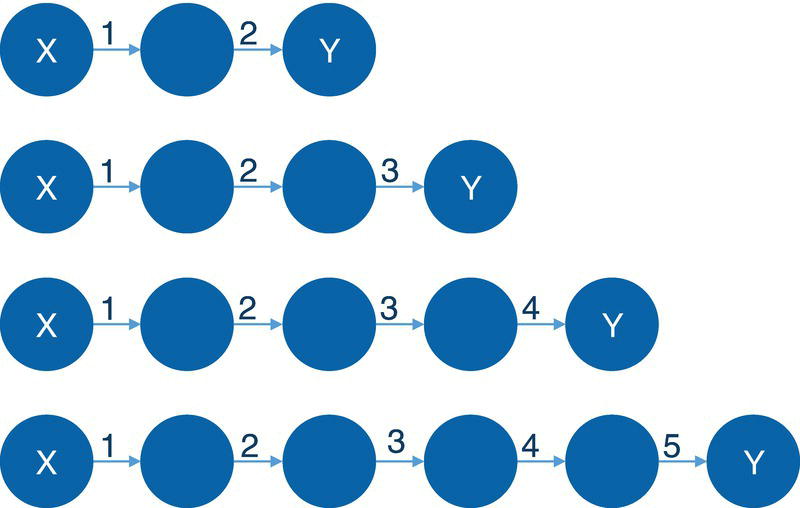
Figure 2.95 Four patterns in a path of sequential transactions.
The option CODE = specifies the code that defines the Function Compiler (FCMP) functions that will be applied to define the query graph.
The option INDUCED = specifies whether to filter matches by using the induced subgraph of the match. If the option is TRUE, proc network keeps only matches whose induced subgraph is topologically equivalent to the query graph. If the option is FALSE, proc network does not filter by using the induced subgraph of the match.
For the nodes, there are two types of filters. The option LINKFILTER = specifies the name of the FCMP function that will be applied for link filters. The option LINKPAIRFILTER = specifies the name of the FCMP function that will be applied for link‐pair filters.
For the nodes, there are also two types of filters. The option NODEFILTER = specifies the name of the FCMP function that will be applied for node filters. The option NODEPAIRFILTER = specifies the name of the FCMP function that will be applied for node‐pair filters.
The option MATCHFILTER = specifies the name of the FCMP function for a filter that is based on a potential match. That means the match is based on any subset of nodes or links or both.
The option MAXMATCHES = specifies the maximum number of matches for the pattern matching algorithm to report in the output tables. This option can be any number greater than or equal to one. If the option is ALL, which is the maximum value that can be represented by a 64‐bit integer, all matches (limited to that maximum number) are reported.
The option MAXTIME = specifies the maximum amount of time to spend in the pattern matching algorithm. The type of time can be either CPU time or real‐time. The type of the time is determined by the value of the TIMETYPE = option in the PROC NETWORK statement. The default value is the largest number that can be represented by a double.
The pattern matching problem involves finding and extracting subnetworks from a larger network that perfectly match certain criteria. In other words, the pattern matching creates subnetwork by querying a large network and selecting all the subnetworks that satisfy a set of predefined rules. Conceptually, the pattern matching method resembles the process of querying a traditional database, selecting only the rows where a criterion is satisfied. In that way, instead of selecting all observations from a table where some criteria, we can think of this process as selecting all subgraphs from the main graph where links and nodes match to a specific pattern. The table in SQL procedures is the main graph, and the where clause in the SQL statement is the filter defined by the pattern on the links and nodes. The observations returned as the outcome of the SQL procedure are the subgraphs returned as the outcome of the pattern matching.
2.9.1 Searching for Subgraphs Matches
Let's consider that the following graph presented in Figure 2.96 exemplifies the searching for subgraph matches. This graph has 19 nodes and 26 links. Initially this graph will be considered as an undirected graph. All the links within this input graph are weighted. The link weight is important when the query graph is defined and searched in the main graph.
The following code describes how to create the links dataset The links dataset has only the nodes identification, specified by the from and to variables, plus the weight of each connection.
data mycas.links;input from $ to $ weight @@;datalines;A B 5 B C 2 C D 3 D B 1 N A 3 A K 2 N K 4 M K 2 L K 1A E 5 E H 1 H A 5 H I 6 H J 4 J I 7 E F 3 E G 2 F G 8B N 5 N O 1 O P 2 P N 1 N Q 5 Q R 1 R S 4 Q S 2;run;
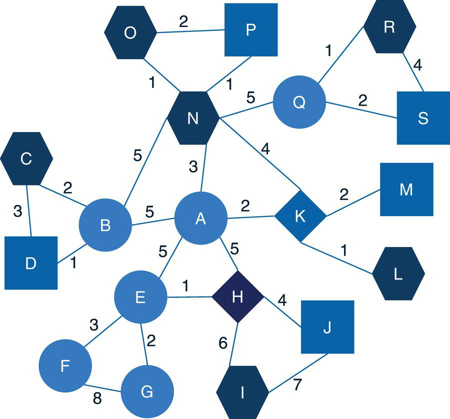
Figure 2.96 The main graph with undirected links.
The following code describes the nodes dataset. In the pattern matching, the nodes are important when the query graph considers some particular nodes attributes. The nodes dataset defines the node identification and the attribute that will be used in the query graph, the shape.
data mycas.nodes;input node $ shape $ @@;datalines;A circle B circle C hexagon D square E circle F circle G circleH diamond I hexagon J square K diamond L hexagon M squareN hexagon O hexagon P square Q circle R hexagon S square;run;
The following code defines the nodes used in the query. The query graph specifies a particular set of nodes and their attributes. For example, this definition specifies that the query graph must have six nodes (1 to 6), where two nodes with square shapes (2 and 6) and another two nodes with hexagon shapes (1 and 5). The other two nodes (3 and 4) could have any shape.
data mycas.nodesquery;input node shape $ @@;datalines;1 hexagon2 square5 hexagon6 square;run;
Finally, the following code defines the links used in the query graph when the pattern matching algorithm searches for the subgraphs. In addition to the set of nodes, the query graph also specifies a particular set of links and their attributes. For example, this definition specifies that the query graph consists of seven links, connecting nodes 1 and 2, 2 and 3, and then 3 and 1. The missing values for the link weights specify that any weight between these nodes is accepted in the pattern matching search. The connection of these three nodes creates a triangle cycle (1→2→3→1). The nodes identification as 1, 2, and 3 means that any triangle cycle within the input graph satisfy the criteria for the query graph, as long as the first node is a hexagon, and the second node is a square. The third node could be of any shape. The links dataset for the query graph defines another triangle cycle, specified by the links between nodes 4 and 5, 5 and 6, and then 6 and 4 (cycle 4→5→6→4). Again, the missing values for the link weights define that any weight between these nodes is accepted by the query graph. Finally, the query graph defines that these two triangle cycles must be connected by a link with a weight of 5. The link between nodes 3 and 4 defines the connection between the triangles with a link weight of 5.
data mycas.linksquery;input from to weight @@;datalines;1 2 .2 3 .3 1 .3 4 54 5 .5 6 .6 4 .;run;
Figure 2.97 shows the query graph defined by the nodes and links datasets associated with the pattern matching. This query graph means that the pattern searched in the main graph consists of two triangles connected by a link with weight of 5. Each triangle must contain a hexagon, a circle, and a square.
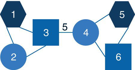
Figure 2.97 The query graph.
As the main graph is defined by the links and nodes datasets, and the query graph is defined by the nodes query and links query datasets, we can invoke the pattern matching algorithm in proc network to search for all subgraphs within the input graph that matches to the pattern specified. The following code describes the process. Notice that, in addition to the nodes and links definitions by using the options NODES = and LINKS =, we also have the definition of the query graph by using the options NODESQUERY = and LINKSQUERY. We specify the variables used to define the main graph by using the statements NODESVAR and LINKSVAR. The option VARS = in the NODESVAR statement specifies the attribute of the nodes that will be used during the pattern matching, which is the shape of the node, defined by the variable shape in the nodes' dataset. Similarly, we need to specify the variables used to define the query graph. Now we use the statements NODESQUERYVAR and LINKSQUERYVAR. The VARS = option in the NODESQUERYVAR statement defines the attributes of the nodes that need to be matched during the search. The variable shape in the nodes query dataset defines the shapes of the nodes comprised in the triangles, hexagon, circle, and square. Finally, the VARS = option in the LINKSQUERYVAR statement defines the attribute of the links that must be matched during the search. The variable weight in the links query dataset defines the link weight of the connection between the two specified triangles as a weight of 5.
proc networkdirection = undirectednodes = mycas.nodeslinks = mycas.linksnodesquery = mycas.nodesquerylinksquery = mycas.linksquery;nodesvarnode = nodevars = (shape);linksvarfrom = fromto = toweight = weight;nodesqueryvarnode = nodevars = (shape);linksqueryvarfrom = fromto = tovars = (weight);patternmatchoutmatchnodes = mycas.outmatchnodesoutmatchlinks = mycas.outmatchlinks;run;
Figure 2.98 shows the summary output for the pattern matching algorithm. It shows the size of the network, 19 nodes and 26 links, the direction of the graph, and the number of matches found along the output tables reported.
The OUTMATCHNODES table presented in Figure 2.99 shows all the matches found, with the association of the query graph node (1 through 6) to the main graph node (A through S). That determines, for this particular match, what role the node in the main graph role plays in the query graph. Finally, this output shows the node attribute used when searching for the matches. The shape of the node plays a key role when the algorithm matches the query graph to the main graph.
As an undirected graph, the number of matches is doubled, as the links in both main and query graphs have both directions. For example, matches 1 and 2 are the same. The only difference is the direction of the links when the pattern matching algorithm searches for the query graph in the main graph. The same happens for the matches 3 and 4. They are exactly the same match with different links directions. Let's consider the first match for example. The nodes C, D, and B represent the first triangle cycle, where one node must be a hexagon (node C), one node must be a square (node D), and the third node can be of any shape. For this particular triangle, node B is a circle. The second triangle cycle in this match is represented by the nodes N, O, and P. Similarly, the triangle must have a hexagon node, which is node N, and a square node, which here could be either node N or node O, as both are hexagons nodes. The third node in the triangle can be of any shape, which means it can be either node N or node O. The last criterion for the pattern match is the link weight between these two triangles cycles. It must be a link with a weight of 5. This link is the connection between nodes B and N. This link will be reported in the output table for the links within the matches. The same concept is applied to the second unique match, the match 3. It is represented by one triangle cycle formed by the nodes O, P, and N (with either node O or N as the hexagon and node P as the square), another triangle cycle formed by the nodes Q, R, and S (with node R as the hexagon and node S as the square) and the connection between these two triangles cycles represented by the link N‐Q with weight of 5.
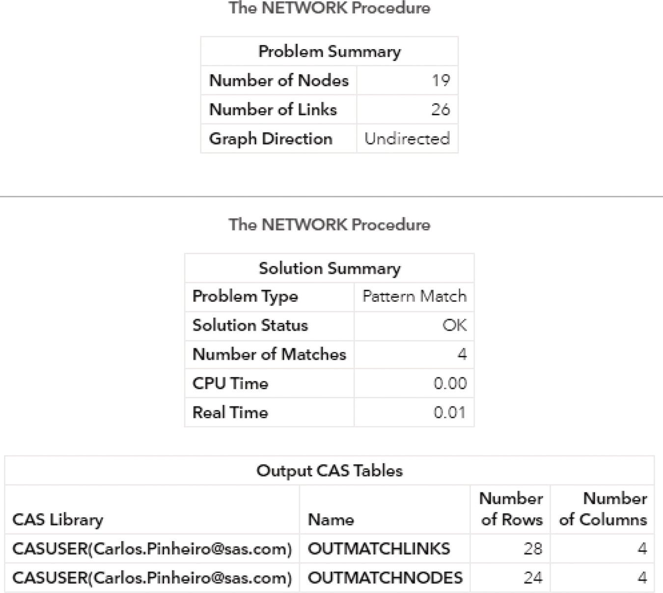
Figure 2.98 Output results by proc network running the pattern matching algorithm.
The OUTMATCHLINKS table presented in Figure 2.100 shows the links between the nodes that represent the matches found.
The matches in the nodes output are associated with the matches in the links output. That means the match 1 in the OUTMATCHLINKS shows the links between all nodes in the match 1 in the OUTMATCHNODES output. The important link though here is the link that represents the connection between the two triangles specified in the query graph. This link in the match 1 is the link between nodes B and N, which must have weight of 5. That is described by line 3 in the output table. The same for the second unique match 3, which is represented by the link between nodes N and Q with link weight of 5. This link is in the output table, but it is suppressed in the picture.
Figure 2.101 shows a graphical representation of the two matches found by the pattern matching algorithm.
Notice that this picture shows only the unique two matches found, matches 1 and 3. Matches 2 and 4 are the same as 1 and 3, only with different links directions. Match 1 is represented by nodes C, D, and B, connected to the nodes O, P, and N. The connecting link between the two triangle cycles is represented by the link (B,N,5). Match 3 is represented by nodes O, P, and N, connected to the nodes R, S, and Q. The connecting link between the two triangle cycles is represented by the link (N,Q,5). This picture also highlights a possible match. The triangle E‐F‐G is connected to the triangle H‐I‐J. The first triangle cycle however doesn't match the criterion of having one square and one hexagon nodes. The second triangle cycle matches that criterion. However, this subgraph also doesn't match the criterion of having a link between the two triangle cycles with weight of 5. The link between them in this subgraph has link weight of 1.
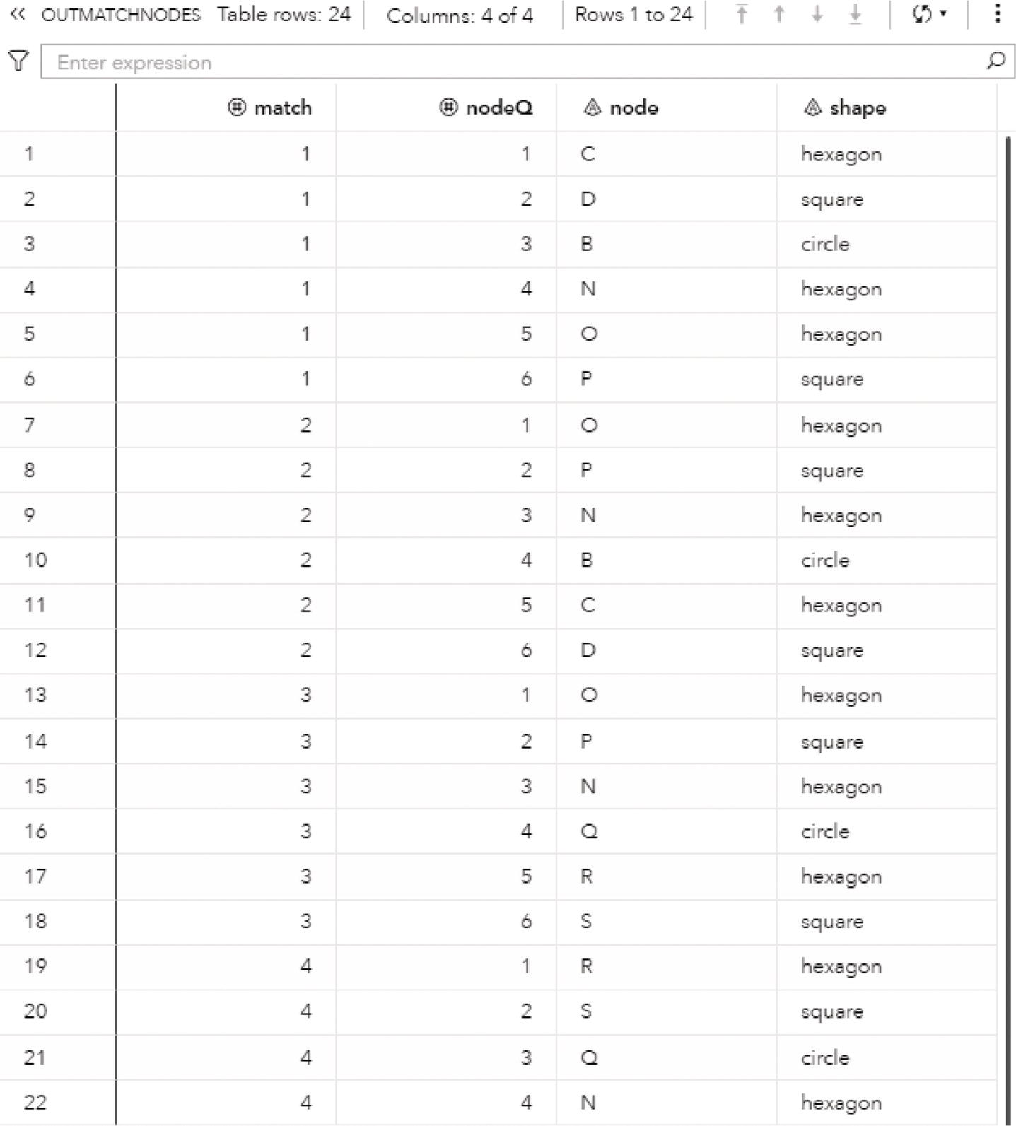
Figure 2.99 Output nodes table for the pattern matching algorithm.
Let's see how the pattern matching works when the graph is defined by directed links. Let's consider the exact same graph definition we used before. The only difference here is that the order of the nodes in the links dataset defines the direction of the link by the from node and the to node. The same is applied for the query links dataset. The links definition in the query links table also defines the direction of the link represented by the variable from and to.
Figure 2.102 shows the main graph but now considering the direction of the links.
As stated before, the direction of the links also affects the query graph. Figure 2.103 shows the query graph considering directed links.
We can invoke proc network to execute the pattern matching algorithm within the defined links and nodes sets, as well as the query links and query nodes sets with a single change to consider a directed graph instead of an undirected one. The following code shows the change in the DIRECTION = option.
proc networkdirection = directed...run;
The OUTMATCHNODES table presented in Figure 2.104 shows the single match found. This match is the same match 1 found on the undirected graph. This match comprises the first triangle cycle formed by nodes C, D, and B, and the second triangle cycle formed by nodes N, O, and P.
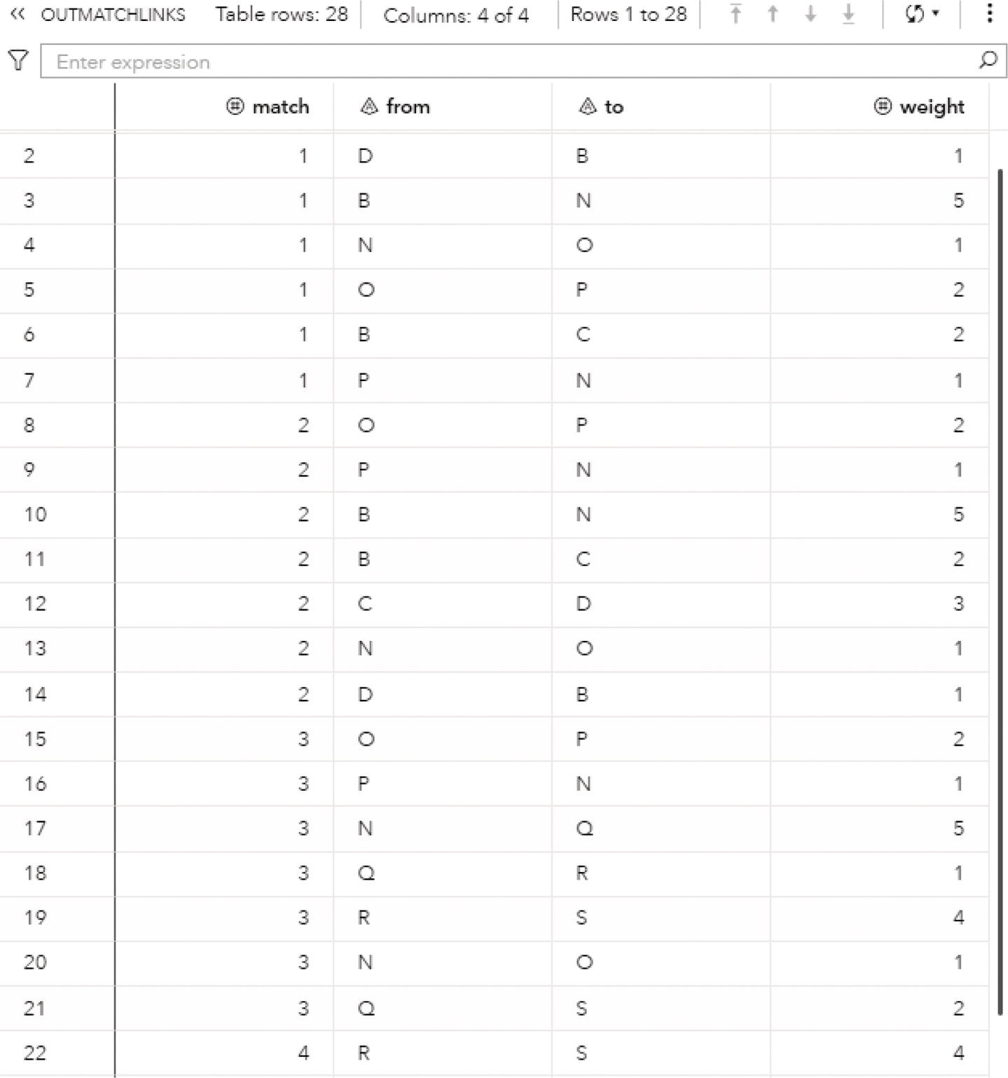
Figure 2.100 Output links table for the pattern matching algorithm.
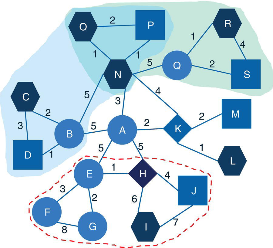
Figure 2.101 Pattern matching outcome.
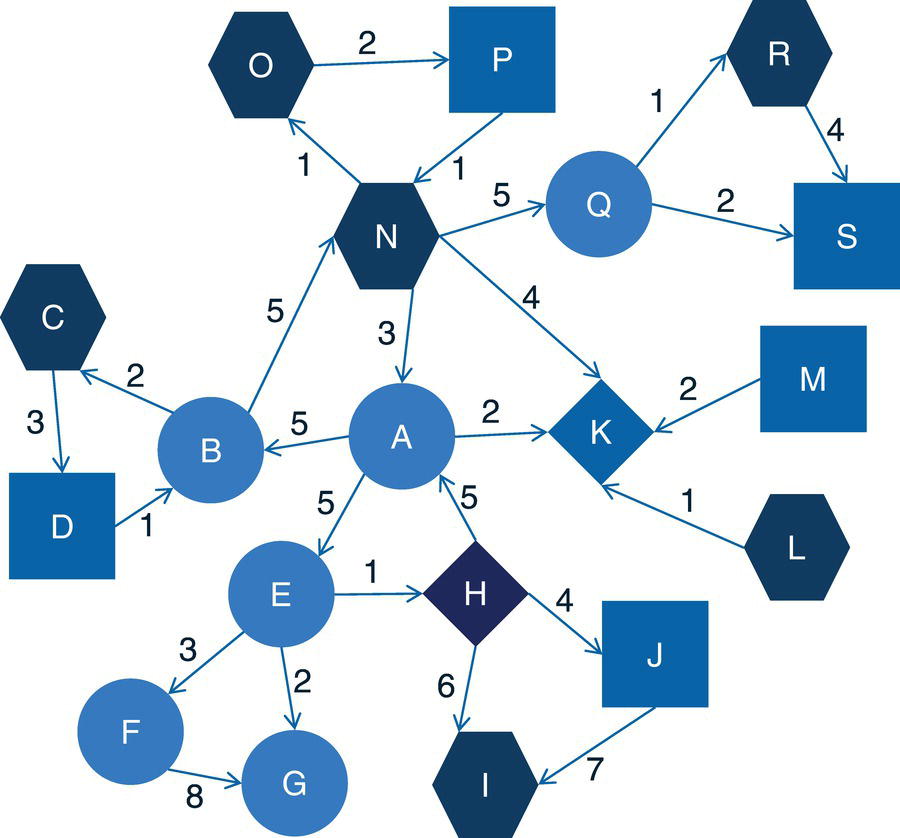
Figure 2.102 The main graph with directed links.
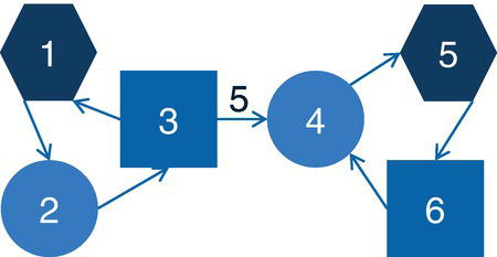
Figure 2.103 The query graph with directed links.
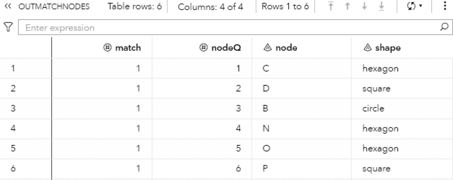
Figure 2.104 Output nodes table for the pattern matching algorithm for a directed graph.
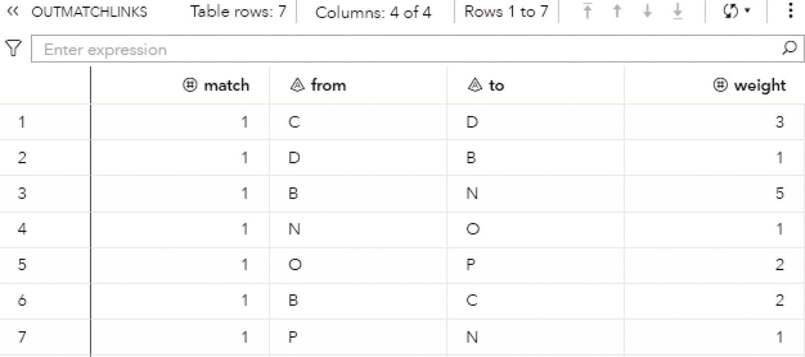
Figure 2.105 Output links table for the pattern matching algorithm for a directed graph.
The OUTMATCHLINKS table presented in Figure 2.105 shows the links between the nodes that represent the single match found. It shows the links that create the two triangle cycles (C→D→B→C and O→P→N→O) along the link that connect them (B→N,5).
Figure 2.106 shows a graphical representation of the single match found by the pattern matching algorithm when running on the directed graph.
Pattern matching is getting more and more attention in network science and analytical modeling, particularly in business applications related to fraud detection and suspicious transactions. This algorithm can be applied to multiple business scenarios, considering different industries.
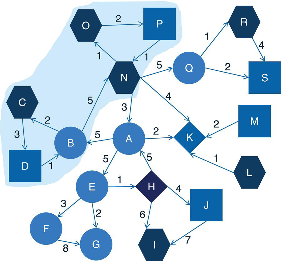
Figure 2.106 Pattern matching outcome on the directed graph.
2.10 Summary
The concept of subgraphs is important in network analysis and network optimization. Many network problems can be divided into smaller problems looking into subnetworks instead of the entire original graph. Also, particularly for large networks, there are multiple distinct patterns hidden throughout smaller groups of actors and relations in the original graph. Analyzing subgraphs instead of the entire graph can, therefore speed up the overall data analysis and make the network outcomes easier to interpret.
Concepts on connected components and how each member of the connected component can reach out to any other member makes this type of subgraph relevant within the network. Some networks don't show many connected components, and if we find some, there should be worth to deeply analyzing them.
The concept of biconnected components is similar to the connected component except for the fact that there is an important actor on it. The articulation point can play a significant role in the network, splitting the network into two or more groups of members. The articulation point plays as a bridge in connecting different groups within the original network and by removing them from the graph, we can completely change the structure of the original network. This role is, therefore, very important, and any articulation point in the network should be further analyzed or closely monitored.
The core, or the k‐core decomposition, is an extremely important concept that divides the original network into groups of nodes based on their interconnectivity. Nodes with a high level of interconnectivity will be gathered into the same k‐core, and nodes with low level of connectivity will be fitted into different cores. This approach allows us to identify groups of individuals or entities within the network that play similarly in terms of relationships. The most cohesive core represents the nodes with the same higher interconnectivity, and the nodes in the less cohesive core will be the nodes with the lower level of interconnectivity or relations. K‐core decomposition has been used in many applications in life sciences, healthcare, and pharmaceutical industries, identifying relevant patterns in diseases spread and contagious viruses.
Reach or ego networks are instrumental when we want to highlight the behavior of a small group of individuals, or even a single one in particular. The reach network represents how many individuals can be reached out from a single person, in one or more waves or connections, and can be important in marketing campaigns when thinking about business, or in terms of the relevance of a node in spreading out something, when thinking about healthcare and life sciences. For example, targeting individuals with a substantial reach network can be effective a marketing campaigns, as well as identifying cells with a great reach network can be effective in terms of possible treatments.
Community detection and analysis is one of the most common and important concepts in subgraphs. Data scientists and data analysts use communities to better understand the network they are analyzing and efficiently identify the nuances of the entire graph in terms of structure and topology. Specially in large networks, the concept of communities can help us in computing network metrics, dividing the overall computation from one single huge graph to multiple smaller subgraphs. Some of the concepts we are going to see in the next chapter, like closeness and betweenness centralities, can be impractical or even infeasible in large networks, but they can make much more sense when computed upon communities. Multiple communities can be detected within large networks, and often they have very different shapes, structures, and patterns of members relationships. Analyzing different communities by different perspectives allows us to define more precise and specific approaches when applying network analysis outcomes. Some communities can be large and dense, some can be large and sparse, some can be small and dense, some small and sparse. Different characteristics implies distinct approaches to not just apply the results but also to interpret the network outcomes.
Network projection is also an important concept to reduce the network size according to some specific characteristics and features. As we saw in this chapter, the network projection reduces a multi‐partition network into a single‐partition network. By doing this, we can select a subset of nodes of interest, segregate them into a small network, and keep their relationships characteristics for a more specific and narrowed network analysis. The network projection can be used from customers‐items relationships to relationships between metabolites and enzymes, and from authorships relations to genes‐diseases correlations, among many other practical applications.
Nodes or graph similarity also has multiple practical applications in science and business. The concept of nodes similarity can be used to compare biological or social networks, and can be used in web searching and to find match in chemical structures. It can also be used to find similar groups of customers from a large network, or more specifically, to identify similar actors practicing any suspicious activity throughout the network over time.
Finally, pattern match has been shown to be useful for many applications. Pattern match perfectly represents the concept of subgraph isomorphism, where the problem is to find a subgraph G ′ of graph G that is isomorphic to graph H. Both graphs G ′ and H must have the same topology. Pattern matching addresses the same problem by searching similar subgraphs within the network based on a defined set of nodes and links attributes. Pattern matching is used to detect fraud in financial institutions, to match DNA sequences in biology applications, or to recognize voice, text, and images in computer science problems. There is an endless number of practical applications that can involve the pattern matching algorithm, whether in full or partially.
The concept of subgraphs is important and will be used in the further chapters, narrowing network centralities computation, guiding network analysis, or determining specific solutions in network optimization.