
1
Concepts in Network Science
1.1 Introduction
Network science is the study of connected things. Things can be represented by people, devices, companies, governments, agencies, bank accounts, etc. Connected can be represented by calls, messages, likes, money transferring, references, geo‐positioning, contracts, etc.
The study of networks has emerged in diverse disciplines as a means of analyzing complex relational data. Every industry, in every domain, has information that can be analyzed in terms of linked data. Network science can be applied to understand different types of spatiotemporal events, from (virus spread to traditional business events such as churn and product adoption in telecommunications and entertainment, service and product consumption in retail industry, fraud or exaggeration in insurance, or money laundering and fraudulent transactions in banking, among many others business scenarios.
Network analysis includes graph theory algorithms that can augment statistical and machine learning modeling. In many practical applications, pairwise interaction between the entities of interest in the model often plays an important role and can be used as input or independent variables in supervised models. Very often they turn out to be one of the best predictors. Network analysis goes beyond traditional unsupervised modeling like clustering and supervised modeling like predictive models. Both supervised and unsupervised models are frequently used to identify hidden patterns in data. However, these models are based on the attributes describing the observations, normally entities. Network science often reveals hidden patterns on the relationship of these entities, rather than on their individual attributes.
Network analysis can be used to understand customers' behavior, highlighting possible influencers within the network, and therefore avoid churn, diffuse products and services, detect fraud and abuse, identify anomalies, and many other business and life science applications. Network analysis applies to a wide range of industries such as communications and media, banking, insurance, retail, utilities, travel, hospitality, transportation, education, healthcare, life science, among many others. It is hard to think about any application, in any industry, that cannot benefit from network analysis.
Network optimization includes graph theory algorithms that can augment more generic mathematical optimization approaches. Many practical applications of optimization depend on an underlying network. Networks also appear explicitly and implicitly in many other application contexts. Networks are often constructed from certain natural co‐occurrence types of relationships, such as among researchers who coauthor articles, actors who appear in the same movie, words or topics that occur in the same document, items that appear together in a shopping basket, terrorism suspects who travel together or are seen in the same location, and so on. In these types of relationships, the strength or frequency of interaction is modeled as weights on the links of the resulting network. Particularly in network optimization, nodes can represent computers, stores, locations, cell towers, bank accounts, vehicles, trains, airplanes, or even a person walking. The occurrence of a transaction involving two nodes can represent a link between them. For example, a truck delivering goods to multiple stores. The stores represent the nodes. The truck going through these multiple stores represents a link between the stores, or the links between the nodes. The weight of these links can be defined by the frequency of the truck's trips between any two stores, the number of goods delivered, or a combination of both. Analogously to the traditional network analysis approach, the network optimization methods can represent nodes and link in the same way but use them differently when distinct optimization algorithms are applied. For example, in the finance industry, bank accounts, individual persons and organizations can represent nodes. All transactions between bank accounts, persons, and organizations can represent link. Money transfers, withdrawals, payments, wires, etc., all represent different types of connections between these nodes, which may have different importance, and thus, different weights. In traditional network analysis, components, cores, or communities of nodes can be detected, revealing groups of accounts, persons, or organizations that are strongly related. Highly weighted links can highlight connections between account, persons, and organizations that are not usual. In network optimization, the same network, based on the same graph representation (bank accounts, individual persons, and organizations as nodes, and transactions as links) can be used differently under distinct optimization algorithms. Cycles, clique, paths, and shortest paths can reveal patterns on the connections that cannot be highlighted by traditional network analysis. Pattern matching can search for a specific group of nodes based on particular types of links among them throughout the entire network, identifying target connections or entities. In the previous example, where stores are nodes and trucks delivering goods are links, network optimization algorithms can search for optimal routes to minimize the time or the distance when trucks are delivering the goods. By adding a depot as a node and a vehicle capacity for the truck, network optimization algorithms can also search for the optimal trips that truck needs to perform when delivering the goods from the depot throughout all the stores.
Somehow, when looking at the problem through a network's perspective, anything can be represented as nodes, and anything can be represented as links. It is just a matter of how the problem will be described by a graph, using nodes and links to represent entities and relationships. Based on this, any problem can be envisioned as a network problem. Perhaps, the network analysis or the network optimization methods will not actually solve the problem, but definitely these methods will help with the solution by highlighting distinct aspects of the entities relationships that cannot be revealed by traditional approaches.
1.2 The Connector
Tensions ran high between American colonists and British soldiers in the spring of 1775. On the morning of April 19th, a few hundred British soldiers set‐off from Boston to capture a cache of arms and arrest some rebel leaders. Marching north into the small towns of Lexington and Concord, the British were astonished to encounter fierce and well‐organized resistance. Soundly beaten, they beat a hasty retreat back to Boston under constant harassment from colonial militia. The nascent rebellion was given a huge boost in confidence. Thus began the war for American Independence from Great Brittan.
How the colonial militia was notified in time and able to assemble ahead of the advancing British troops is a story well known to American schoolchildren, many of whom have read or perhaps even memorized the Henry Wadsworth Longfellow poem called “The Midnight Ride of Paul Revere.”
On the afternoon of April 18, 1775, a boy who worked at a livery stable in Boston overheard one British army officer say to another something about “hell to pay tomorrow.” The stable boy ran with the news to Boston's North End to the home of a silversmith named Paul Revere. Revere listened to the news very seriously, as it was not the first rumor to come his way that day. Earlier, he had been told of an unusual number of British officers gathered on Boston's Long Wharf, talking in hushed tones. British crewmen had been spotted moving quickly in the boats tethered beneath the HMS Somerset and the HMS Hoyne in Boston Harbor. Several other sailors were seen on shore that morning, running what appeared to be last‐minute errands. Revere and his close friend, Joseph Warren, became more and more convinced that the British were about to make the major move on the long‐rumored march to the town of Lexington, northwest of Boston, to arrest the colonial leaders John Hancock and Samuel Adams, and then on to the town of Concord to seize the stores of guns and ammunition that some of the local colonial militia had stored there.
Revere and Warren decided they had to warn the communities surrounding Boston that the British were on their way, so that local militia could be roused to meet them. Revere was spirited across Boston Harbor to the ferry landing at Charlestown. He jumped on a horse and began his “midnight ride” to Lexington. In two hours, he covered 13 miles. Along the way, in every town he passed through, he knocked on doors and spread the word, telling local colonial leaders of the oncoming British, and telling them to spread the word to others. The news spread like a virus as those informed by Paul Revere sent out riders on their own, until alarms were going off throughout the entire region. The word was in Lincoln, Massachusetts, by 1 A.M., in Sudbury by3 A.M., in Andover, 40 miles northwest of Boston, by 5 A.M., and by nine in the morning had reached as far west as Ashby, near Worcester. When the British finally began their march toward Lexington on the morning of April 19, 1775, their attack into the countryside faced an organized and fierce resistance. In Concord that day, the British were confronted and soundly beaten by the colonial militia, and from that exchange came the war known as the American Revolutionary War.
Revere rode his horse through the night alerting militia men of the approaching army. Hundreds quickly turned up ready to fight the heavily armed British troops. However, a young man named William Dawes also rode out of Boston the same night with the same message. Starting earlier than Revere, and riding through more populous towns along a more westerly route, Dawes could have been expected to arouse even more rebels. But he didn't. The few militia men who responded to Dawes turned up too late to be of much use.
Paul Revere is an essential figure in American History. William Dawes is but a footnote. Both men carried the same message into towns where the people had equal motivations. One started a word‐of‐mouth epidemic; the other was mostly ignored. But why?
Malcolm Gladwell, proposes an answer to this question in his 1999 book named The Tipping Point, How Little Things Can Make a Big Difference. According to Gladwell, Paul Revere was a special type of person, a connector. William Dawes was a 26‐year‐old shoemaker. He rode through towns knocking on random doors and shouting that the British were coming. But people in these towns didn't know who he was, didn't have confidence that his message represented an immediate threat. They didn't see their neighbors doing anything so they went back to bed, figuring they would check it out in the morning. Paul Revere on the other hand was well known. He was a successful businessman who at age 40 had for years been at the center of events in and around Boston. When Paul Revere rode into a town he didn't knock on a random door but went straight to the local militia commanders. Opening their doors in the middle of the night and recognizing Paul Revere on the doorstep, they quickly acted, alerted their neighbors, and spread the word. Revere alerted enough of the right people, so the alarm reached the tipping point. The answer is that the success of any kind of social epidemic is heavily dependent on the involvement of people with a particular and rare set of social gifts. Revere's news tipped and Dawes's didn't because of the differences between the two men.
This story is a classic example of how connectors are essential to get an idea to tip. But what can this history lesson from 235 years ago tell us about today's fast‐moving, high‐technology marketplace? Instead of riding around on horses shouting to each other, we use mobile phones, e‐mail, and social network sites. But these special people, the connectors, are still with us. The technology may have changed but connectors still influence our behavior, and they are worth paying attention to.
Connectors know lots of people, many times the number of people the average person knows. But they also know essential facts about people. Chances are you know someone like this, someone that seems to know everyone and stops to talk wherever they go, but it isn't all small talk. Connectors know what to talk about with the people they meet. If you tell a connector about your hobby, they can give you the names of several people who share that interest. Tell them about a problem you have, and they will give you the names of people who can be helpful. Tell them about a great new product and a connector will spread the word. Research has shown that most people have at one time found a job because a connector put them in contact with someone they did not know who helped them get the job. Connectors play a vital role in our social networks.
The impact of connectors to a small neighborhood business is quite obvious. A local restaurant owner would give his best table to a guy who is very influential in the neighborhood while some average person will likely find himself seated near the kitchen. This local restaurant owner may realize that there are more customers on nights when this influential guy shows up and may also observe other customers saying hello to the influential guy and asking him to join them. People stay longer and spend more money when he is around. Owning a local restaurant may be a high‐risk business and the presence of one person like that influential guy can determine if the business will tip toward profitability.
However, big corporations, for example communications service providers, are not a local restaurant. Business managers can't personally know millions of customers. Yet the impact of connectors can be vital clues to what others will be doing in the future. Losing a connector to a competitor can represent an increase in churn numbers for the next quarter. On the other hand, seduce a connector away from your competitor and other customers may follow. Have a new service? Get the word to a connector and see how fast it spreads throughout his social network.
But how does a communications service provider know that someone is a connector? Companies can't just put a check box on the service application that asks: “Are you a connector: yes or no?” Unlike gender, connector is not a binary status. Connectors could be expected to be heavy service users, but just accumulating call minutes and numbers of messages is not a good indicator, because these calls and messages may be only assigned to a small number of people. Looking at the number of people someone calls won't help either. A taxi driver may talk with hundreds of people a month, but if he's just arranging pick‐ups, he's not a connector. That is when network analysis comes into play, computing centrality measures that can reveal the different roles people have within the social network and highlighting the well‐connected customers. Different centralities describe different behaviors, representing something different to the company. Most likely, a combination of different centralities like closeness, betweenness, influence, degree, PageRank, etc., can better reveal the connectors within the communications network, allowing the company to avoid influential people to move away to the competitors, which eventually will be followed by other customers.
1.3 History
Social network analysis considers social life as relations between individuals. The different behaviors within a network are critical to understanding social connections, and more importantly, the implications of those behaviors on communities. One of the most impactful implications within social relations is how someone can influence other people to do similar actions. For example, in the fashion industry, influencers affect how followers dress. In the corporate world, business and thought leaders influence how people manage teams or even companies. Sports idols influence fans to not just support their clubs but also consume products they advertise. In academia, respectful authors influence other scholars on their teaching and research assignments. The list of examples of influence in different environments is virtually endless.
Traditional methods of data analysis and analytical modeling usually consider individual attributes from all observations when exploring the data and searching for hidden patterns. For example, what is the customers' average purchase behavior? How many customers use certain products or services? How long do they remain customers? Do they delay their payments? How long on average? All these questions are about the individuals, looking at their attributes or characteristics. Network analysis focuses on the attributes and characteristics of the relations rather than of the individuals. Individuals' attributes can also be important, and they are also considered in the analysis. However, most often, the attributes of the relations between individuals reveal more hidden patterns. Even when individuals' attributes are considered, they are analyzed from a relationships' perspective. For example, what do the relations of specific entities look like? Specific entities are defined by entities attributes. But the focus of the analysis is on the relationships of those entities.
1.3.1 A History in Social Studies
In the 19th century, Émile Durkheim, a French sociologist, published The Rules of Sociological Method. Durkheim describes a theory of sociology as the science of social facts. The article explores the phenomena that is created by interactions between individuals. These relations describe a reality that is independent of any individual actor. He defined the social fact as any way of acting, whether fixed or not, capable of exerting an external constraint over the individual. The social fact is a phenomenon, which is general over the whole of a given society whilst having an existence of its own, independent of its individual manifestations.
In the 20th century, George Simmel, a German sociologist and philosopher, was one of the first scholars to think about explicitly describing social network terms. He examined how third parties could affect the relationship between two individuals. He examined how organizational structures were needed to coordinate interactions in large groups.
One of the first examples of network research was described in 1922. John Almack, a professor at Stanford, published a paper that anticipated the development of the sociometric instrument. He wrote “The Influence of Intelligence on the Selection of Associates.” In this study, he asked California elementary school children, grades 4–7, to identify the classmates that they wanted as playmates. One question for example was, “If you had a party, which boy from your class would you invite?” Almack then correlated the IQs for the choosers and the chosen and examined the hypothesis that choices were homophilous.
In 1926, Beth Wellman, an American psychologist, was also focused on homophilous choices among pairs of individuals. Wellman recorded pairs of individuals who were observed as being together frequently. She noted additional attributes such as students' height, grades, gender, age, IQ, score in physical coordination tests, and degree of introversion versus extroversion (based on teachers' ratings). She studied 63 boys and 50 girls who were enrolled in Lincoln Junior High. She then studied homophily with respect to all these traits. Wellman then examined whether interactions were homophilous or not.
In 1928, Helen Bott, a Canadian developmental psychologist, performed an ethnographic approach to examine the behavior of the play activities among preschool children at the nursery attached to the University of Toronto. She identified five types of interactions: talking to one another, interfering with one another, watching one another, imitating one another, and cooperating with one another. She then used the focal sampling to observe one child each day. Bott organized her data into matrices and discussed the results in terms of linkages between individuals. It was a brand‐new approach, largely based on the network analyses that are used today.
In 1933, Elizabeth Hagman, an American psychologist, observed interactions within a particular timeframe and interviewed children to measure their recollections of their interactions earlier in that term. This study was called “The Companionships of Preschool Children.” Those studies established an important approach for network analysis, particularly in defining how to link individual attributes to interactions, such as IQ, gender, social class, and so on. She highlighted the difference in the observational approaches and the individuals' own accounts of their patterns of interactions. Hagman emphasized the ability to take into account the many different types of interactions between individuals, and the fact that sometimes the linkage attributes might say more about the individuals than the individuals' attributes.
In 1933, The New York Times reported on the new science of psychological geography, which “aims to chart the emotional currents, cross currents, and under currents of human relationships in a community.” Jacob Moreno, a Romanian American psychiatrist and psychosociologist, is considered by many as one of the fathers of social network analysis, with the graphical social network of interactions between school children in The New York Times. He developed the sociogram and presented it to the public at an April 1933 convention of medical scholars. Moreno claimed that “Before the advent of sociometry no one knew what the interpersonal structure of a group ‘precisely’ looked like.” The sociogram was a representation of the social structure of a group of elementary school students. Moreno analyzed interconnections among 500 girls in the State Training School for Girls and also interconnections of students in two New York City schools. He observed that many relationships were non‐reciprocal, and as a result, many individuals were isolated. The boys were friends of boys, and the girls were friends of girls, with the exception of one boy who said he liked a single girl. This network representation of social structure was so intriguing that it was printed in The New York Times on April 3, 1933. The sociogram has found many applications and has grown into the field of social network analysis. Moreno initially referred to his research as psychological geography, but later changed the name to sociometry. In 1938 he started the Sociometry journal. His work was largely theoretical, and his social networks were more illustrative than mathematical representations. Moreno recognized that, and began working with Paul Lazarsfeld, a mathematical sociologist from Columbia University. Lazarsfeld developed a probabilistic model of a social networks, which was published in the first volume of Sociometry.
Between 1935 and 1939, Theodore Newcomb studied the women of Bennington College. He observed that when women were exposed to the relatively liberal referent group of fellow students and faculty, they became more liberal. “Becoming radical meant thinking for myself and, figuratively, thumbing my nose at my family. It also meant intellectual identification with the faculty and students that I most wanted to be like.”
In 1950, Festinger studied the influence of dorm room location and found that individuals were more likely to associate with those who were similar to them. In this particular case, similar means proximity. Festinger proposed that those who were physically close to each other were more likely to form positive associations. The study showed that the dorm room arrangements could influence the formation of both weak and strong relationships between the students.
After the 1950s, networks were less evident in social psychology and more evident in sociology. Developments in the last few decades included much attention to concepts such as the strength of weak ties and the small worlds. These findings were mainly important to social behavior studies. In the last decade several business applications, including a huge database, were developed based on the “social” study of networks.
In 1998, David Krackhardt and Kathleen Carley introduced the idea of a meta‐network with the PCANS Model. They suggested that “All organizations are structured along these three domains, individuals, tasks, and resources.” Their paper introduced the concept that networks are interrelated and occur across multiple domains. This field has grown into another sub‐discipline of network science called dynamic network analysis.
More recently other network science efforts have focused on mathematically describing different network topologies. Duncan Watts reconciled empirical data on networks with mathematical representation, describing the small‐world network. Albert‐László Barabási and Reka Albert developed the scale‐free network, which is a loosely defined network topology that contains hub vertices with many connections, and grow in a way to maintain a constant ratio in the number of the connections, versus all other nodes. Although many networks, such as the internet, appear to maintain this aspect, other networks have long tailed distributions of nodes that only approximate scale free ratios.
1.4 Concepts
In mathematics, specifically in graph theory, a graph is a structure represented by a set of objects, where these objects are connected in pairs. Objects can describe any type of entity, like a person, a company, a bank account, or a country. The connections between these pairs of objects can describe any type of relationship, like text messages, contracts, money transfers, or international trades. These objects can be named differently, according to the domain knowledge, or even different authors. The same for those connections. Objects can be referred to as nodes, vertices, or points. Connections can be referred to as links, edges, arcs, or lines. In this book, the nomenclature used will be nodes and links. A node will be an individual unit in the graph, and the link will be an interaction between a pair of nodes.
A network, or a graph G, is then defined as a pair G = (N, L), where N is a set of nodes and L is a set of links. The nodes i and j of a link (i, j) are also called endpoints of the link. The link is commonly referred to as join nodes i and j or to be incident on i and j. This pair of nodes i and j is also referred to as adjacent if there is a link (i, j) connecting them. A node can be isolated in the graph, which means, it is not joined to any other node, or has no link incident to it. A node can be connected to itself, representing an auto relationship. A graph can be undirected or directed. A directed graph means that all the links within the graph have a source node (origin) and a sink node (destination). The link (i, j) can be represented by i → j. An undirected graph has links with no directions, which means a link (i, j) can represent i → j or j → i. In undirected networks, the association between two nodes is reciprocal. That is, if node i is connected to node j, it is implied that node j is also connected to node i. In other words, a link between two nodes implies a two‐way reciprocal association. Friendship is a good example of an undirected network, where two folks are friends to each other, reciprocally. In directed networks, this reciprocal association does not exist. If a link exists pointing from node i to node j, it does not mean that node j also points to node i. If node j also points to node i, another link would need to represent this relationship. Authorship is a good example of a directed network, where an author of a paper refers to many other papers, and therefore, to many other authors. That reference doesn't imply that the referred authors also refer to the original author of the paper.
Finally, both nodes and links can have attributes to represent some particular characteristics of the entity or the relationship. For example, in a telecommunications network, the nodes can represent customers, and one important characteristic is the average revenue per user (ARPU). The ARPU will be the node weight. The link can represent a call between two customers or a text message, or even a multimedia message. Each of these connection types has a different importance for the carrier, and then can be weighted accordingly. For example, the call can be weighted by the number of minutes, the text message can be weighted by the number of characters, and the multimedia message can be weighted by the megabytes. Each one of these measures will be the link weight.
Figure 1.1 shows directed and undirected links, as well as nodes and links with different weights.
The link weight is a crucial measure in most of the network analysis and network optimization algorithms. The link weight can represent the importance or the frequency of the connection between two nodes in network analysis, affecting the way to calculate some centrality metrics like influence, eigenvector, PageRank, closeness and betweenness. The link weight also can represent the cost, the demand, or the capacity of the connection between two nodes in network optimization. Cost, demand, or capacity affect the calculation of some network optimization algorithms like shortest path, traveling salesman problem, vehicle routing problem, minimum spanning tree, minimum‐cost network flow and maximum flow.
Nodes and links can be represented as input data sets, in a sequential data fashion, or as matrices. For example, Figure 1.2 shows a graphical representation of a small network.
The directed graph presented before can be represented by a matrix, as shown in Figure 1.3. In this representation, all nodes can be connected to all other nodes, including the self‐relation. When a link occurs connecting a pair of nodes, the matrix's cell assigned to these two nodes is flagged. The flag can represent the frequency, the link weight, or any information that represents the importance of that connection.
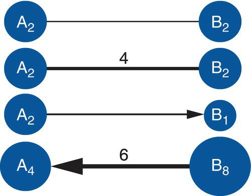
Figure 1.1 Directed and undirected links with weighted nodes.
In addition to the matrix representation, the previous graph can be also described as a table. This representation only shows the pairs of nodes that are connected by a link. This type of representation may save a substantial amount of space, either in memory or disk, particularly when representing large networks. For example, the matrix representation of the directed graph, containing 8 nodes and 10 links uses 64 cells (8 nodes × 8 nodes). The table representation uses on 10 cells or observations, exactly the 10 links connecting the 8 nodes throughout the network. Figure 1.4 shows the table representation for that directed graph.
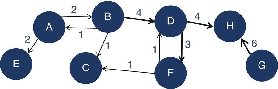
Figure 1.2 Representation of a directed graph with weighted nodes and links.
Matrices to represent networks can frequently be very sparse, especially in large networks, as not all nodes are connected to all other nodes. A large storage may be required to represent a network, even though the majority of the possible combinations of source and sink nodes will be empty. Tables represent networks by only using the existing relations, which can not only save storage but can also be highly effective to process, read and write.
1.4.1 Characteristics of Networks
Two factors have a great impact on the way the information flows between the nodes within a network.
- Topology: the shape of the network, where one node cannot pass information to another unless they are connected.
- Time: the timing for the connections, where a node cannot pass information before it has received it from another node.
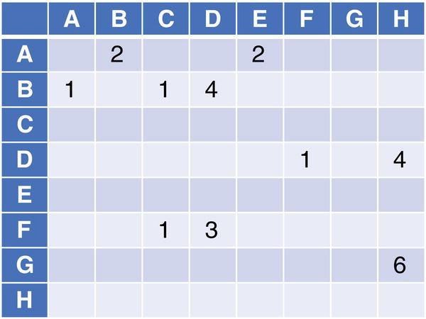
Figure 1.3 A matrix representation for a graph.
Two key features of the network topology consider the way the nodes are connected throughout the network.
- Connectivity: Describes how nodes in one part of the network are connected to other nodes in another part of the network. It is the possible paths between one node to another perhaps taking intermediates along the way.
- Centrality: Describes how some nodes are connected to other nodes in particular locations of the network. It describes how central the node is within the network.
Connectivity and centrality are mostly translated by the connections between the nodes within the network. Neighborhood and degree are two metrics that describe how connected a node is.
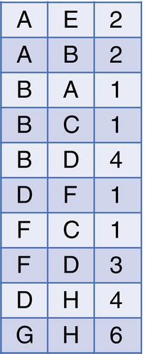
Figure 1.4 A table representation for a graph.
- A neighborhood N for a node is the set of its immediate connected nodes.
- Degree is the network metric k i of a node representing the number of other nodes in its neighborhood. It is, in practice, the number of distinct connected nodes that a particular node n has.
- Degree‐out represents the number of nodes that a node n points out (outbound interactions).
- Degree‐in represents the number of nodes that a node n is pointed to (inbound interactions).
1.4.2 Properties of Networks
Some of the network metrics can be used to describe the topology of the network. For example, the metric density describes how connected the network is considering the total number of existing links and the number of possible links that network could have. The number of possible links in the network derives from the total number of nodes. It accounts for all possible connections that all the nodes within the network could have. The size of the network is calculated based simply on the number of existing nodes. The average degree indicates how balanced or well distributed the connections are throughout all nodes within the network. Most of the networks tend to present a power law distribution, where a few nodes have a great number of connections, while the majority of the nodes present only a few connections. The simple network metrics can initially describe the main characteristics of the network and its topology. The average path length describes how close the nodes within the network are to each other. The average path length recalls the concept of six degrees of separation, where there are up to six people between any two people in the world. Some dense networks may have low average path length, indicating nodes are close to each other in terms of reachability, and some networks may present higher average path length, showing that nodes may require multiple steps to reach out to other nodes within the network. Diameter is another important measure to describe the topology of the network. It measures the longest shortest path between all pairs of nodes within the network. This measure describes the possible longest distance between a pair of nodes within the network. Clustering coefficient is a measure that describes how connected a node's neighborhood is. It considers the number of existing connections between a node's neighbors and the possible number of connections these neighbors could have. A well‐connected neighborhood means that the information flowing through it may be more persistent than an information flowing throughout a sparse or low‐connected neighborhood.
The density of a network is defined as the ratio of the number of the existing links to the number of possible links. L is the number of existing links within the network and N is the number of existing nodes.
The size of a network is simply the number of nodes N.
The average degree is the sum of degree k for all nodes divided by the number of existing nodes N within the network.
The average path length is calculated by finding the shortest path between all pairs of nodes divided by the total number of pairs.

The diameter of a network is the longest path considering all shortest paths within the network, where u and v represent a pair of nodes, and d(u, v) is the path that connects nodes u and v, no matter the number of steps it takes, or the number of nodes in between them. For example, node u is connected to node v passing through nodes i, j, and k. The path connecting nodes u and v is u → i → j → k → v. The distance d(u, v) between nodes u and v is 4.
Both metrics, average path length, and diameter are metrics to describe how wide and spanned the network is.
The clustering coefficient of a node is the ratio of the existing links connecting a node's neighbors to each other to the maximum possible number of links between those node's neighbors.
The clustering coefficient C i for a node n i considers all existing links l jk between the set of neighbors N i for the node i, and all possible links these neighbors can have, k i (k i − 1). In a directed graph, the link l jk differs from the link l kj . Then, considering the set of neighbors N i of node i and the set of existing links L between those neighbors, the clustering coefficient C i of node i is:

In an undirected graph, the links l jk and l kj are identical. Then, for a particular node n i with k i neighbors, the number of possible links is ![]() . The clustering coefficient of node i in an undirected graph is:
. The clustering coefficient of node i in an undirected graph is:

Those basic network metrics give an overall description of the network's topology and how nodes are connected and close to each other. Chapter 3 presents a full spectrum of network centrality metrics to better describe the main characteristics of the network, its nodes, and its links.
1.4.3 Small World
Mark Sanford Granovetter is an American sociologist and professor at Sanford University. In 1973, he published a paper in the American Journal of Sociology called “The Strength of Weak Ties.” The idea of the strength of the weak ties is probably one of the most important concepts in social network analysis, and that study is one of the top sociology papers published in recent decades.
Granovetter argues that those weak ties observed within social networks actually might be more advantageous in politics or in seeking employment than the expected strong ties. It happens because the weak ties enable individuals to reach more individuals than the strong ties. In fact, by having more weak ties, a person can reach out to more people than by having a few strong ties.
In social network analysis, this is one of the most important concepts. The idea of weak ties is about reachability. It states that, in most of the cases, it is more important to have lots of weak connections than a few strong ones. The reachability from having lots of connections, even though it is based on weak ties, is greater than the reachability from having strong links but only a small number of them.
Some of Granovetter's observations include: the presence of weak ties often reduces path lengths or distances between any two individuals within the network. Short paths enable the information diffusion to speed up throughout the network. This is actually the concept of closeness and betweenness. Weak ties shorten the distances between nodes within the network. The presence of weak ties in the network creates multiple paths between nodes, gathering them closer to each other.
One of the most famous concepts in network analysis is the one assigned to small worlds. The concept basically argues that the world is small because there are a few nodes separating any pair of two distinct nodes. In social networks, it means that a person can reach out to any other person in the world by contacting a fixed number of other persons in the path.
Two possible graphs, almost at opposite ends of a spectrum, are random graphs and regular graphs. A small world can be thought of as existing between a random graph and a regular graph.
The small world concept is assigned to the concept of six degrees of separation. It states that there is an average number of people (or nodes) in the world (or the network) separating any two persons. This number changes according to the network under analysis.
The concept of small worlds is associated with the concepts of random graphs and regular graphs, as well as with clustering coefficients and network diameter. There are basically three types of graphs: regular, small‐world, and random. They differ based on the probability that any two nodes are connected within the network. Figure 1.5 shows representations of these three distinct types of graphs.
In random graphs, each pair of nodes i, j has a link with an independent probability p. For example, Figure 1.6 shows a graph with 16 nodes and 19 links.
With 16 nodes, this graph has 120 possible links, which is represented by how many combinations are possible from 16 nodes taken 2 at a time. The possible number of combinations is described by the following formula:
where n represents the number of items, here 16 nodes, and r represents the number of items being chosen at a time, here 2 nodes to create a link. The total number of possible links is then:
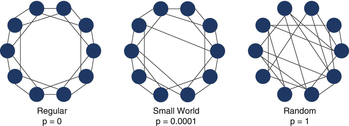
Figure 1.5 Representation of the three types of graphs, regular, small world, and random.
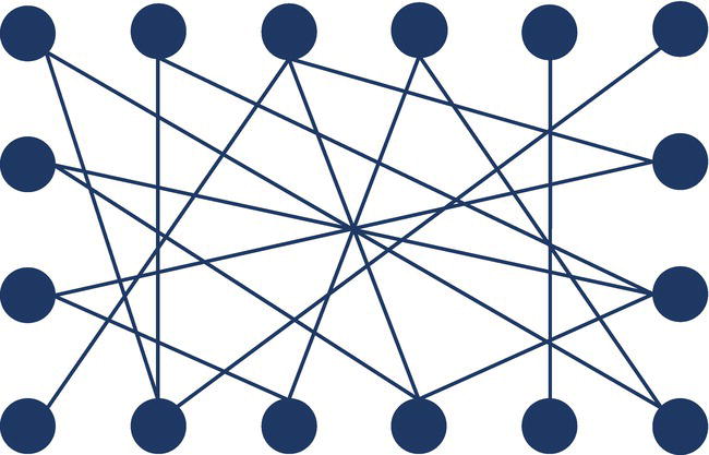
Figure 1.6 Random graph.
However, this graph has only 19 existing links. The probability of a link, or a node being connected to another node, is 0.16 (19 existing links divided by the 120 possible links). In other words, the probability of a node being connected to another node is 0.16.
In random graphs, the presence of a link between A and B and a link between B and C will not influence the probability of a link between A and C. Therefore, in a random graph, nodes have an independent probability of being connected.
In regular graphs, each node has the same number k of neighbors, which is represented by the degree. Figure 1.7 shows a graph with 6 nodes and 9 links.
With 6 nodes, this graph has 15 possible links.
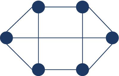
Figure 1.7 Regular graph.
This graph has only 9 existing links. The probability of any two nodes being connected to each other is 0.6 (9 links by 15 possible).
In this regular graph, all nodes have a degree k of 3, which means, every node within the network is connected to exactly three other nodes. They all have the same number of neighbors (k = 3). In regular graphs, each node has the same number of connections.
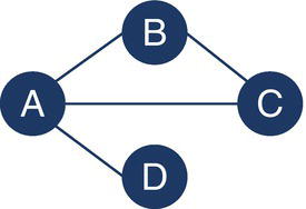
Figure 1.8 Graph representing four legislators working in committees.
In 1998, Duncan Watts, an American sociologist and professor at University of Pennsylvania, and Steve Strogatz, an American mathematician and professor at Cornell University, introduced a network metric called clustering coefficient. Clustering coefficients is a measure of how close a node and its neighbors are from being a clique or a complete graph within a larger network. The clustering coefficient of a node is the number of actual connections across its neighbors as a percentage of the possible connections between them. The concept of small worlds is associated with the clustering coefficient network measure. It measures how connected a node's neighborhood is.
Suppose that four legislators are working in committees. It is an undirected graph, which means that if legislator A serves with B in a committee, then legislator B serves with A. Figure 1.8 describes this small network of legislators.
Following the previous concept, four legislators (nodes) in a network creates six possible connections. Legislator A has three neighbors. They have 1 link out of 3 possible (1/3). Legislator B has two neighbors. They have 1 link out of 1 possible (1/1). Legislator C has two neighbors. They have 1 link out of 1 possible (1/1). Legislator D has one neighbor. There is no possible link in this case (0/0). The clustering coefficient is computed for each node by dividing the number of existing connections among its neighbors by the number of possible connections.
Graph diameter is the longest shortest path between any two nodes within the network. Figure 1.9 shows four graphs with the same number of nodes, but a different number of links.
The first graph has a diameter of 3, the second graph has a diameter of 4, the third graph has a diameter of 5, and finally the fourth and last graph has a diameter of 7. The last graph on the right has a larger diameter because it takes, at most, seven links to travel from one node to another. The two highlighted nodes at the bottom in the graph are actually not well‐connected, which makes the diameter for this graph the largest among the four graphs presented.
As the longest shortest distance between any two nodes in the network, the graph diameter is associated with the degrees of separation. It shows how many nodes or steps are in between any pair of nodes in the network.
The small world is basically the idea of six degrees of separation. It is the number of steps or links needed to connect any node to another one within the network. The main idea behind the concept of the small world is that the number separating any pair of nodes is often small. That means, observed networks present lower diameters than expected.
In 1967, Stanley Milgram, an American social psychologist and former professor at Yale and Harvard Universities, published an important study, “The Small‐World Problem,” which generated great publicity. This publicity was supported primarily by several research projects that were conducted simultaneously and that focused on the concept that the world was becoming highly interconnected. Notice that this experiment took place in 1967. It is not difficult to imagine now the impact this concept had, viewing the possible types of relationships people could establish with the use of different devices, technologies, and geographies.
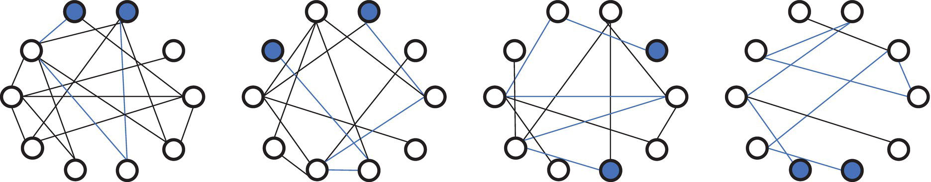
Figure 1.9 Four graphs with same number of nodes and different number of links.
In this experiment, individuals were asked to reach a particular individual target by passing a message along a chain of acquaintances. For successful chains, the average number of acquaintances was five people, which means, six steps. However, in that study, many of those chains were not actually completed. The idea of the small world is that most networks have smaller diameters than expected, which means that there are fewer people than expected between any two people in the network.
Stanley Milgram conducted some experiments to examine the average length of the path for particular networks. The main objective of these experiments was to suggest that the human communities were not too big. One individual could reach any other one by some maximum number of steps or, in other words, by a certain number of intermediate individuals between them. Indeed, the research outcomes suggested that the networks were characterized by short paths among the nodes considering the number of those intermediate steps. One experiment was associated with the famous phrase “six degrees of separation.” However, Milgram himself had never used this term to reference his experiment.
Milgram's experiment intended to highlight the likelihood that two randomly selected people would know each other, regardless of the length of the path, or in other words, the number of steps (nodes and links) between them. This is certainly one way to solve the small‐world problem. A straight method to solve the small‐world problem is by calculating the average length of the path connecting any two distinct nodes inside the network. The Milgram experiment ultimately created a particular algorithm to calculate the average number of links that connected any two nodes.
The idea behind finding out the number of degrees that separate people in a network has triggered further concepts about how people behave inside the network rather than the number of connections that they have. In terms of business, it is more important to know how each individual behaves inside the network than it is to know how many connections there are among people – that is, of prime importance is their correlated nodes through their connected links.
Georg Simmel, a German sociologist, and philosopher was influential in the field of sociology. According to Simmel, the premise that social ties are primarily based on viewing components as isolated units, those components are better understood as being at the intersection of particular relations and deriving their defining characteristics from the intersection of these relations. He argues that society itself is nothing more than a web of relations.
He wrote: “The significance of these interactions among men lies in the fact that it is because of them that the individuals, in whom these driving impulses and purposes are lodged, form a unity, that is, a society. For unity in the empirical sense of the word is nothing but the interaction of elements. An organic body is a unity because its organs maintain a more intimate exchange of their energies with each other than with any other organism; a state is a unity because its citizens show similar mutual effects.”
This statement is an argument against the premise that a society is just a bunch of individuals who react individually and independently to particular circumstances according to their personal desires. Based on his belief that the social world is found in interactions rather than in an aggregation of individuals, Simmel argued that the primary work of sociologists is to study patterns among these interactions rather than to study the individual motives.
Simmel wrote in the same study: “A collection of human beings does not become a society because each of them has an objectively determined or subjectively impelling life‐content. It becomes a society only when the vitality of these contents attains the form of reciprocal influence; only when one individual has an effect, immediate or mediate, upon another, is mere spatial aggregation or temporal succession transformed into society.”
1.4.4 Random Graphs
Let's examine four different graphs. They all have the same number of nodes, 12, but different a number of links. Let's assume that N represents the number of nodes, p represents the probability that a pair of nodes is connected, and k represents the average degree for the network, or the number of neighbors of a node. In this analysis, let's examine the size of the largest connected cluster within the four graphs, the diameter (longest shortest path between nodes) of the largest cluster, and the average path length between all nodes within the network. Figure 1.10 shows these four different graphs.
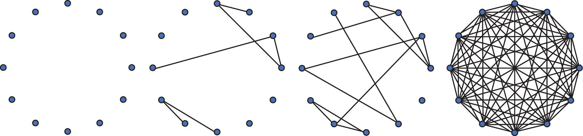
Figure 1.10 Four graphs with same number of nodes but different number of links.
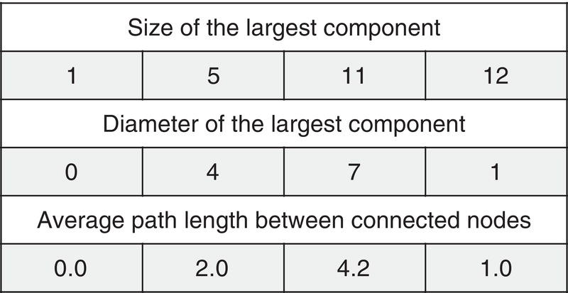
Figure 1.11 Largest component, diameter, and average path for the four graphs.
All four graphs have N = 12. The first graph has p = 0 and k = 0, which means no probability to have nodes connected and then no neighbors for all nodes. The second graph has p = 0.09 (6 existing links divided by 66 possible links) and k = 0.9 (11 total degree divided by 12 nodes). The third graph has p = 0.18 (12 existing links divided by 66 possible links) and k = 2 (24 total degree divided by 12 nodes). Finally, the four graph has p = 1 (as a complete graph, 66 existing links divided by 66 possible links) and k = 11 (k ≈ N).
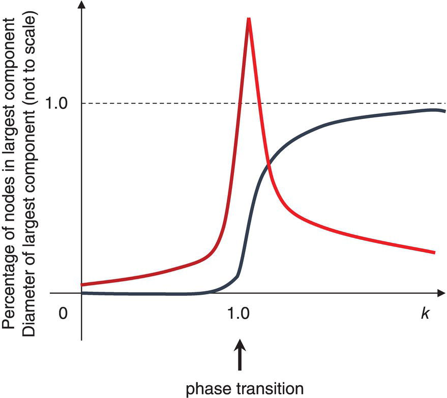
Figure 1.12 Ratio of the size of components and the diameter.
The size of the largest component in graph 1 is 1, in graph 2 is 5, in graph 3 is 11, and in graph 4 is 12. The diameter for graph 1 is 0, in graph 2 is 4, in graph 3 is 7, and in graph 4 is 1. Finally, the average path length between connected nodes in graph 1 is 0, in graph 2 is 2, in graph 3 is about 4, and in graph 4 is 1. Figure 1.11 summarizes these measures.
When k < 1, there are small, isolated clusters, the diameter is small, and there are short path lengths. That means, If the average number of connections is small, the network is shaped by isolated nodes. When k = 1, giant components may appear, there is a peak on the diameter, and path lengths can be very high. That means, If the average number of connections is equal to one, the network topology can be assigned to a huge single group. When k > 1, almost all nodes are connected into a single cluster, diameter shrinks to almost 1 step, and path lengths are short. That means, finally, if the average number of connections is greater than one, the network is shaped by high density, where almost all nodes are connected. Figure 1.12 shows the relation between k to the size of the clusters and diameters.
If connections between people can be modeled as a random graph, and because an average person can easily know more than one person (k >> 1), we live indeed in a small world. The path length between connected nodes would be calculated as ![]() .
.
That brings us back to the concept of six degree of separation. I know someone, who knows someone, who knows someone, who knows someone, who knows someone, who knows someone, who knows you!
1.5 Network Analytics
This book covers network analytics in basically three different approaches. The technical aspects of network analytics are covered in Chapters 2–4. Chapter 5 shows some case studies where network analytics were crucial to solve business problems.
Chapter 2 focuses on the subgraphs, emphasizing a set of algorithms to identify subgraphs and compute some measures about them. For example, it begins by describing how to identify connected components and biconnected components from a major network. Then it moves to how to detect communities by using different algorithms and distinct approaches. It covers how to compute k‐cores, an alternative from community detection. Reach network, an especially useful subnetwork, mostly used in marketing campaigns, is also covered. Network projection is described as a way to identify multiple types of subgraphs from a main graph considering different scenarios. Node similarity is not exactly a subgraph detection, but it is included in Chapter 2 as this algorithm may result in a set of nodes, which can be considered as a subgraph. Chapter 2 finishes with pattern matching, a critical network algorithm in detecting fraud and suspicious transactions from a main graph based on a query graph.
Chapter 3 focuses on the network metrics as a method to evaluate and identify the different roles the nodes can play within a network. Network metrics, or centralities, is also a method to measure the importance of the nodes within the network considering different aspects, like number of connections, strength of the relationships, how central the nodes are in the network, how they may control the information flow, or how influential they can be with other nodes within the network. Degree, influence, clustering coefficient, closeness, betweenness, eigenvector, PageRank, hub, and authority are the centrality measures covered in Chapter 3.
Chapter 4 emphasizes the network optimization area, describing algorithms that aim to minimize or maximize objective functions considering a set of resources, demands, constraints, supplies, or costs. This chapter covers algorithms to find cliques and cycles, compute linear assignment, calculate minimum‐cost network flow, find minimum cuts, identify minimum spanning tree, find paths and shortest paths, compute transitive closure, solve traveling salesman problems, vehicle routing problems, and identify topological sort.
All examples in this book are created using two main procedures in SAS Viya. NETWORK and OPTNETWORK procedures provide a substantial set of network analysis and network optimization algorithms. All algorithms presented in Chapter 2 are available in the NETWORK procedure. Some of them are also available in the OPTNETWORK procedure. All centralities presented in Chapter 3 are available in the NETWORK procedure as well. Finally, all the optimization algorithms presented in Chapter 4 are available in the OPTNETWORK procedure, and some of them are also available in the NETWORK procedure.
There are plenty of materials describing the SAS Viya architecture and how the in‐memory distributed engine works. However, this is not part of the scope of this book. What is important to mention here is that both NETWORK and OPTNETWORK procedures can run in single machines, multiple machines, and in multithreaded executions. Some algorithms run only in single machine mode. Some can use multiple machines, even though each machine requires a global view of the input data, which means, links and nodes, subset of nodes, query graphs, etc. Some algorithms in multiple machines require only a portion of the input data. In this case, the input data is shuffled between machines and then it is randomly distributed across multiple cores. Some algorithms require no data movement, and then the original input data is directly distributed across multiple machines.
In both NETWORK and OPTNETWORK procedures, some algorithms are sensitive to the order in which the data is loaded. Due to the in‐memory distributed engine, just reading input data tables in the same order at each algorithm invocation is not guaranteed. When the order of the nodes or links is different in different executions, the final result may change. By default, both NETWORK and OPTNETWORK procedures ensure that each invocation, considering the same machine configuration and parameter settings, will produce the same final result. However, there is a performance cost for that. The option DETERMINISTIC=FALSE allows both procedures to improve performance, but the final results might differ. Sometimes the difference is only a permutation of identifiers, sometimes it may be an alternative local solution.
1.5.1 Data Structure for Network Analysis and Network Optimization
Relationships in network are mutually exclusive. That means, considering a pair of nodes i and j, a link may or may not connect them. As a result, storing every single relationship among all nodes in a network produces redundant information that the network procedures do not need to perform network analysis and network optimization. In this case, both network analysis and network optimization procedures do not use an adjacency matrix as an input data table. Instead, it uses only the unique elements to represent nodes and links. One example is, if there are nodes with no links, or nodes have no weights, the input data table to represent the nodes is not required for network analysis and network optimization. The data input table to represent the links suffices. The nodes representation can be derived from the links representation.
The NODES= option in both NETWORK and OPTNETWORK procedures defines the data table that contains the list of nodes in the graph. This data table is used to assign node attributes, for example, its labels and weights. The nodes dataset may contain the following variables:
- node: the node label (can be numeric or character).
- weight: the node weight (must be numeric).
The LINKS= option in both NETWORK and OPTNETWORK procedures defines the data table that contains the list of links in the graph. A link is represented by pair of nodes, which can be seen as from source or origin node, and to sink or destination node in directed graphs, or simply from and to nodes in undirected graphs with no differentiation on the direction of the link. The links dataset may contain the following variables:
- from: the from node (can be numeric or character).
- to: the to node (can be numeric or character).
- weight: the link weight (must be numeric).
- auxweight: the auxiliary link weight (must be numeric).
For both nodes and links, additional columns can be read in using the VARS= option. For example, if the nodes in the graph represent customers, an additional column describing their average revenue may be defined and can be read into the node's dataset by the network analysis and network optimization procedures. Analogously, if the links in the graph represent several types of connections between customers like calls, text messages, or multimedia messages, the type of connection can be specified in the links dataset and be read into the network procedure. An example would be VARS=(revenue) or VARS=(type). The VARS= option is used to define additional attributes to be read into the network procedures. Similarly, the option VARSOUT= is used to write additional attributes for both nodes and links into the final results. If this option is not used, all columns specified in the option VARS= are written to the final datasets.
Both NETWORK and OPTNETWORK procedures assume some reserved words for nodes and links attributes. For example, if the nodes dataset has a column named node to identify the nodes and a column named weight to identify the node weight, there is no need to use the NODESVAR= statement to define NODE=node and WEIGHT=weight. The same concept applies to the links dataset. If there is a column named from to define the source node, a column named to to define the sink node, and a column named weight to identify the link weight, there is no need to use the LINKSVAR= statement to define FROM=from, TO=to and WEIGHT=weight.
1.5.1.1 Multilink and Self‐Link
A multigraph is a graph that allows multiple links between nodes. Usually, the links describe different types of relationships or distinct spatiotemporal representation. For example, customers can be represented by nodes in a graph, and multiple types of connections between customers like calls, texts, and multimedia texts can be represented by multiple links. If all types of connections between nodes are summarized into a single link, or there are no multiple types of connections between pairs of nodes, the graph is called a simple graph, or simply a graph. Both NETWORK and OPTNETWORK procedures can execute on simple graphs or multigraphs. In order to run on multiple links between the same pair of nodes, the option MULTILINKS= must be specified. If the option is TRUE, multiple links between a single pair of nodes will be processed individually. If the option is FALSE, the multiple links between the same pair of nodes will be aggregated into one single link that uses the minimum of each attribute value. In that case, the multigraph is transformed into a simple graph. By default, both network procedures work with multigraphs (MULTILINKS=TRUE).
A self‐link is a link for which the from node and to node are the same. It represents an auto relationship. Sometimes the self‐link is confusing or simply does not make any sense. But in some cases, it does. A network representing relationships between employees working in multiple projects with multiple roles might be the case. Employees are represented by nodes. Links represent the hierarchy on the report. If employee (node) A reports to the manager (node) B, there is a link from A to B. However, it might be the case where B also work in the same project, so, B reports to itself in that graph representation. Both NETWORK and OPTNETWORK procedures can work with self‐links. The option SELFLINKS= specifies is the network procedure must remove the self‐links or not before invoking any algorithm. If the option is TRUE, self‐links are allowed. If the option is FALSE, self‐links are removed. By default, both network procedures work with self‐links (SELFLINKS=TRUE).
1.5.1.2 Loading and Unloading the Graph
Some of the network tasks can be time consuming, particularly when large graphs are involved. Substantial time can be spent simply loading the graph into memory before the network procedure can actually invoke any analysis or optimization algorithm. Particularly for large graphs, where loading the input data tables to represent nodes and links can be computationally expensive, and a series of analysis will be performed upon the same network, loading this graph into memory can be beneficial. The LOADGRAPH statement reads the input data tables and stores a standard representation of the graph in memory. The graph identifier is saved in a macro variable called _NETWORK_, or in an output data table created by using the option OUTGRAPHLIST=. A variable named graph stores the graph identifier. This in‐memory graph can be referenced in the network procedure by using the GRAPH= option, by specifying the graph identifier stored in the macro variable or in the output table.
When referencing an in‐memory graph in the network procedure by using the option GRAPH=, sometimes additional data structures are required depending on the algorithm invoked. When that happens, there is an additional one‐time expense on the first execution of this algorithm. However, subsequent calls can then use these data structures directly. For this reason, a first call that includes the GRAPH= option to some algorithms can sometimes take longer than subsequent calls.
Multiple graphs can be loaded into memory at the same time. In order to better manage graphs loaded into memory, there is also an option to unload them from memory when needed. The UNLOADGRAPH statement deletes an in‐memory graph and its persistent data structures.
1.5.2 Options for Network Analysis and Network Optimization Procedures
The PROC NETWORK statement invokes the network analysis procedure, and the PROC OPTNETWORK statement invokes the network optimization procedure. The following options work most of the time for both procedures and specify how both procedures will process the graphs, identify subgraphs, compute centralities, and solve optimization problems.
The option DETERMINISTIC= specifies whether to enforce determinism when running the network algorithms. When the option is TRUE, each invocation produces the same final result. If the option is FALSE, the same final results are not guaranteed.
The option DISTRIBUTED= specifies whether to use a distributed graph when running network analysis and network optimization algorithms. When the option is FALSE, a distributed graph is not used. When the option is TRUE, the graph can be distributed throughout multiple machines and some algorithms can use that distribution to reduce the running time.
The option GRAPH= specifies the in‐memory graph to use when the input graph is loaded into memory to be used in multiple executions.
The option DIRECTION= specifies the direction of the input graph. When the option equals to DIRECTED, the input graph is processed considering directed links, where each link (i, j) has a direction defined in the links input data table. It determines how the information flows through the nodes over that link. For example, considering the link (i, j), the information can flow only from node i to node j, and not node j to node i. Node i is called the source node, and node j is called the sink node. When the option equals to UNDIRECTED, the input graph is processed considering undirected links, where each link (i, j) has no determined direction. In this case, the information can flow from node i to node j, and from node j to node i.
The option LINKS= specifies the input data table that contains the graph link information. The option NODES= specifies the input data table that contains the graph node information. The option NODESSUBSET= specifies the input data table that contains the graph node subset information.
The option OUTLINKS= specifies the output data table to contain the graph link information along with any results from the algorithms that calculate metrics on links. The option OUTNODES= specifies the output data table to contain the graph node information along with any results from the algorithms that calculate metrics on nodes.
The option LOGFREQUENCYTIME= controls the frequency in number of seconds for displaying iteration logs for some algorithms. This option is useful for computationally intensive algorithms as it can show how the algorithms progress over time.
The option LOGLEVEL= controls the amount of information that is displayed in the log. The option NONE turns off all messages to the log. BASIC displays a brief summary of the algorithmic processing. MODERATE displays a moderately detailed summary of the input, output, and algorithmic processing. AGGRESSIVE displays a more detailed summary of the input, output, and algorithmic processing.
The option NTHREADS= specifies the maximum number of threads to use for multithreaded processing. Some of the algorithms can take advantage of multicore machines and can run faster when the number is greater than 1. Algorithms that cannot take advantage of this option use only one thread even if the number is greater than 1.
The option STANDARDIZEDLABELS specifies that the input graph data are in a standardized format. The option STANDARDIZEDLABELSOUT specifies that the output graph data include standardized format.
The option TIMETYPE= specifies whether CPU time or real time is used for each algorithm's MAXTIME= option when applicable. The value CPU specifies units of CPU time. The value REAL specifies units of real time.
1.5.3 Summary Statistics
In both NETWORK and OPTNETWORK procedures, it is possible to compute some important summary statistics about the graph before executing the network analysis or the network optimization algorithms. The SUMMARY statement calculates various summary statistics for the graph and its nodes. Two main categories of summary statistics are created. The first one is based on the entire graph. The second one is based on the nodes and links of the graph. The summary statistics about nodes and links are appended to the output nodes and the output links data tables specified in the options OUTNODES= and OUTLINKS=. The summary statistics about the graph are reported in the data table specified in the OUT= option in the SUMMARY statement. The output columns may differ according to the direction of the input graph.
The option OUT= specifies the output data table in the SUMMARY statement that reports the summary statistics for the graph. This output table contains the following columns:
- nodes: the number of nodes in the graph.
- links: the number of links in the graph.
- avg_links_per_node: the average number of links per node.
- density: the number of existing links in the graph divided by the number of possible links in a complete graph.
- self_links_ignored: the number of self‐links that are ignored.
- dup_links_ignored: the number of links removed in multilink aggregation.
- leaf_nodes: the number of leaf nodes.
- singleton_nodes: the number of singleton nodes.
The summary statistics also reports information about the connectedness of the graph by using the CONNECTEDCOMPONENTS and BICONNECTEDCOMPONENTS options within the NETWORK and OPTNETWORK procedures. When using the options CONNECTEDCOMPONENTS or BICONNECTEDCOMPONENTS, additional statistics are reported to the summary output data table. For an undirected graph, the following columns are added:
- concomp: the number of connected components in the graph.
- biconcomp: the number of biconnected components in the graph.
- artpoints: the number of articulation points in the graph.
- isolated_pairs: the number of isolated pairs of nodes.
- isolated_stars: the number of isolated stars.
For a directed graph, the following columns are added:
- concomp: the number of strongly connected components in the graph.
- isolated_pairs: the number of isolated pairs of nodes.
- isolated_stars_out: the number of isolated outward stars.
- isolated_stars_in: the number of isolated inward stars.
Similarly, the summary statistics can also produce statistics about the shortest paths in the graph by using the SHORTESTPATH= option within the NETWORK and OPTNETWORK procedures. When using the option SHORTESTPATH=, the following columns are added to the summary output data table:
- diameter_wt: the longest weighted shortest path distance in the graph.
- diameter_unwt: the longest unweighted shortest path distance in the graph.
- avg_shortpath_wt: the average weighted shortest path distance in the graph.
- avg_shortpath_unwt: the average unweighted shortest path distance in the graph.
When using the option CLUSTERINGCOEFFICIENT, the summary statistics can add the number of triangles of an undirected graph. A triangle is identified by a set of three distinct nodes where each node is a neighbor of the other two. The CLUSTERINGCOEFFICIENT option adds the following column to the summary output data table:
- triangles: the total triangle count of the graph.
The OUTNODES= option specifies the output table containing the summary statistics for the nodes in the graph. The following columns are appended to the output data table:
- sum_in_and_out_wt: the sum of the link weights from and to the node.
- leaf_node: 1, if the node is a leaf node; otherwise, 0.
- singleton_node: 1, if the node is a singleton node; otherwise, 0.
- isolated_pair: the identifier, if the node is in an isolated pair; otherwise, missing (.).
- neighbor_leaf_nodes: the number of leaf nodes connected to the node.
When the options CONNECTEDCOMPONENTS and BICONNECTEDCOMPONENTS are used, the following columns are added to the output data table. For an undirected graph:
- isolated_star: the identifier, if the node is in an isolated star; otherwise, missing (.).
For a directed graph:
- isolated_star_out: the identifier, if the node is in an isolated outward star; otherwise, missing (.).
- isolated_star_in: the identifier, if the node is in an isolated inward star; otherwise, missing (.).
When the option SHORTESTPATH= is used, the summary statistics include the calculation of the eccentricity of a node. This measure reports the longest of all possible shortest path distances between a particular node and any other node in the graph. The following columns are added to the output data table. For an undirected graph:
- eccentr_out_wt: the longest weighted shortest path distance from the node.
- eccentr_out_unwt: the longest unweighted shortest path distance from the node.
For a directed graph
- eccentr_in_wt: the longest weighted shortest path distance to the node.
- eccentr_in_unwt: the longest unweighted shortest path distance to the node.
The OUTLINKS= option specifies the output table containing the summary statistics for the links in the graph. When the options CONNECTEDCOMPONENTS and BICONNECTEDCOMPONENTS are used, the following columns are added to the output data table. For an undirected graph:
- isolated_pair: the identifier, if the link is in an isolated pair; otherwise, missing (.).
- isolated_star: the identifier, if the link is in an isolated star; otherwise, missing (.).
For a directed graph:
- isolated_star_out: the identifier, if the link is in an isolated outward star; otherwise, missing (.).
- isolated_star_in: the identifier, if the link is in an isolated inward star; otherwise, missing (.).
The summary statistics are always a good approach to better understand the main characteristics of the input graph before beginning a deep analysis of the main graph and invoking network analysis and network optimization algorithms.
1.5.3.1 Analyzing the Summary Statistics for the Les Misérables Network
As a first step in evaluating the network topology in some networks, and in order to better understand the output from the summary statistics, let's take the Les Misérables network presented in Figure 1.13.
The Les Misérables network is an undirected graph, where it represents all the actors who play scenes together throughout the move. As the actors play multiple scenes together during the movie, the number of these scenes is used to create the link weight. The network is small, with 77 nodes (actors) and 254 links (distinct pairs of actors playing scenes together).
The following code invokes proc. network to execute the summary statistics on the Les Misérables network. The SUMMARY statement considers all possible summary statistics, calculating the biconnected components, the connect components, the clustering coefficient, the diameter of the network, the finite path, and the shortest path.
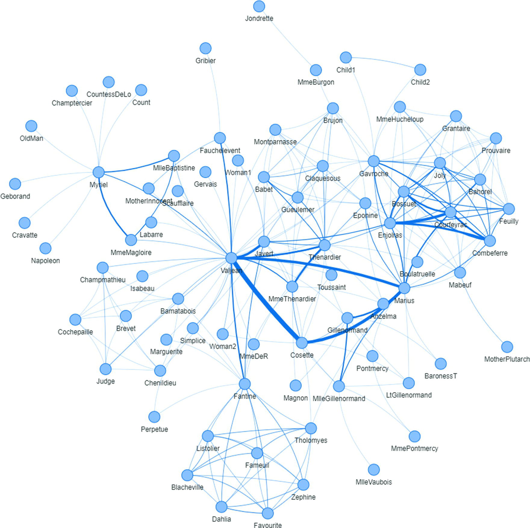
Figure 1.13 Les Misérables network.
proc networkdirection = undirectednodes = mycas.lmnodeslinks = mycas.lmlinksoutnodes = mycas.outnodessummaryoutlinks = mycas.outlinkssummary;nodesvarnode = nodevars = (label)varsout = (label);linksvarfrom = fromto = toweight = weight;summarybiconnectedcomponentsconnectedcomponentsclusteringcoefficientdiameterapprox = bothfinitepathshortestpath = bothout = mycas.summary;run;
Figure 1.14 shows the summary results reported by proc. network when running the summary statistics. It shows the size of the network, with 77 nodes and 254 links. The summary statistics are computed considering the graph with undirected links. Three output tables are produced by the summary statement, one for the nodes, one for the links, and the last one for the summary metrics.
Figure 1.15 shows the SUMMARY output table, consisting of summary metrics for the network, such as the number of nodes and links, the average number of links per node, the number of links divided by the number of nodes, the number of self‐links within the network that were ignored, the number of links that were removed by the multilink aggregation, the number of leaf nodes, and the number of singleton nodes. Leaf nodes are simply external nodes, sometimes called outer or terminal. Simply put, are the nodes with degree of 1. Singleton nodes, sometimes referred to as singleton graphs, are nodes with no links, or nodes isolated in the network.
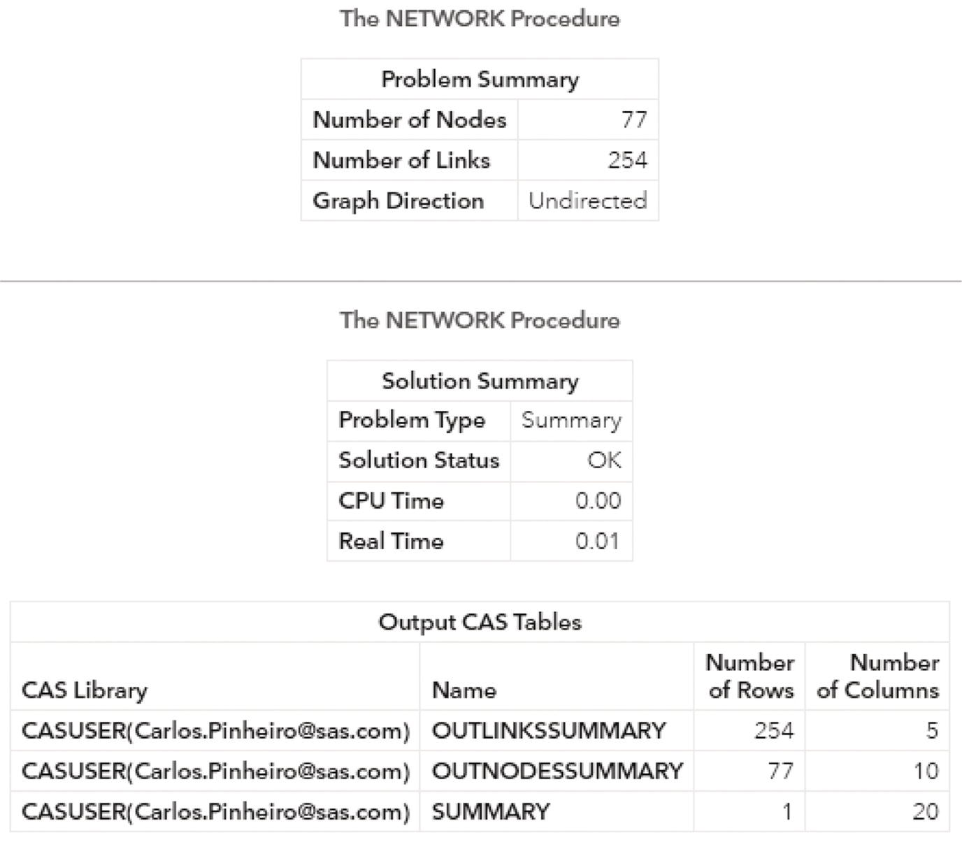
Figure 1.14 Summary statistics results.
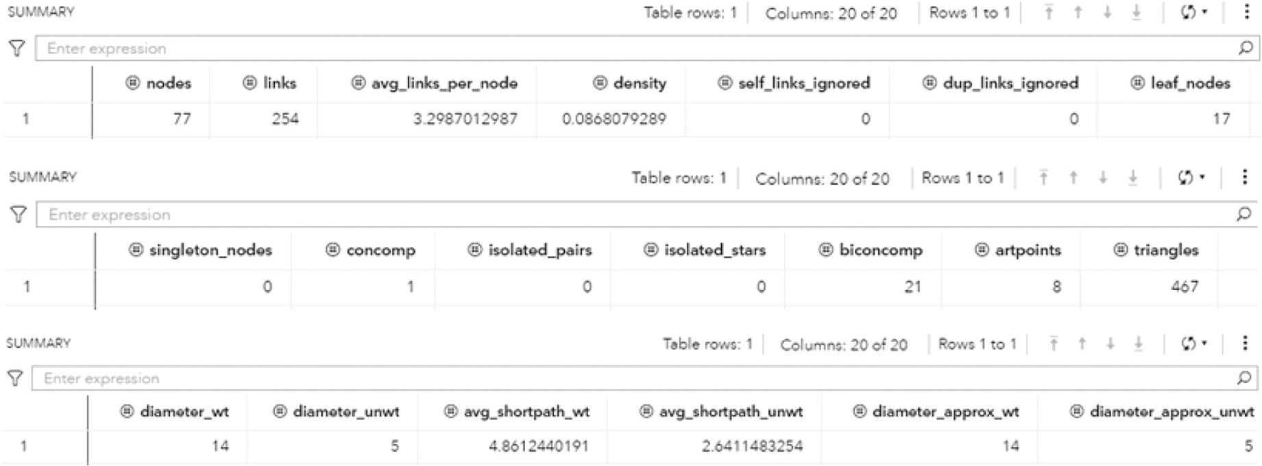
Figure 1.15 Summary statistics for the Les Misérables network.
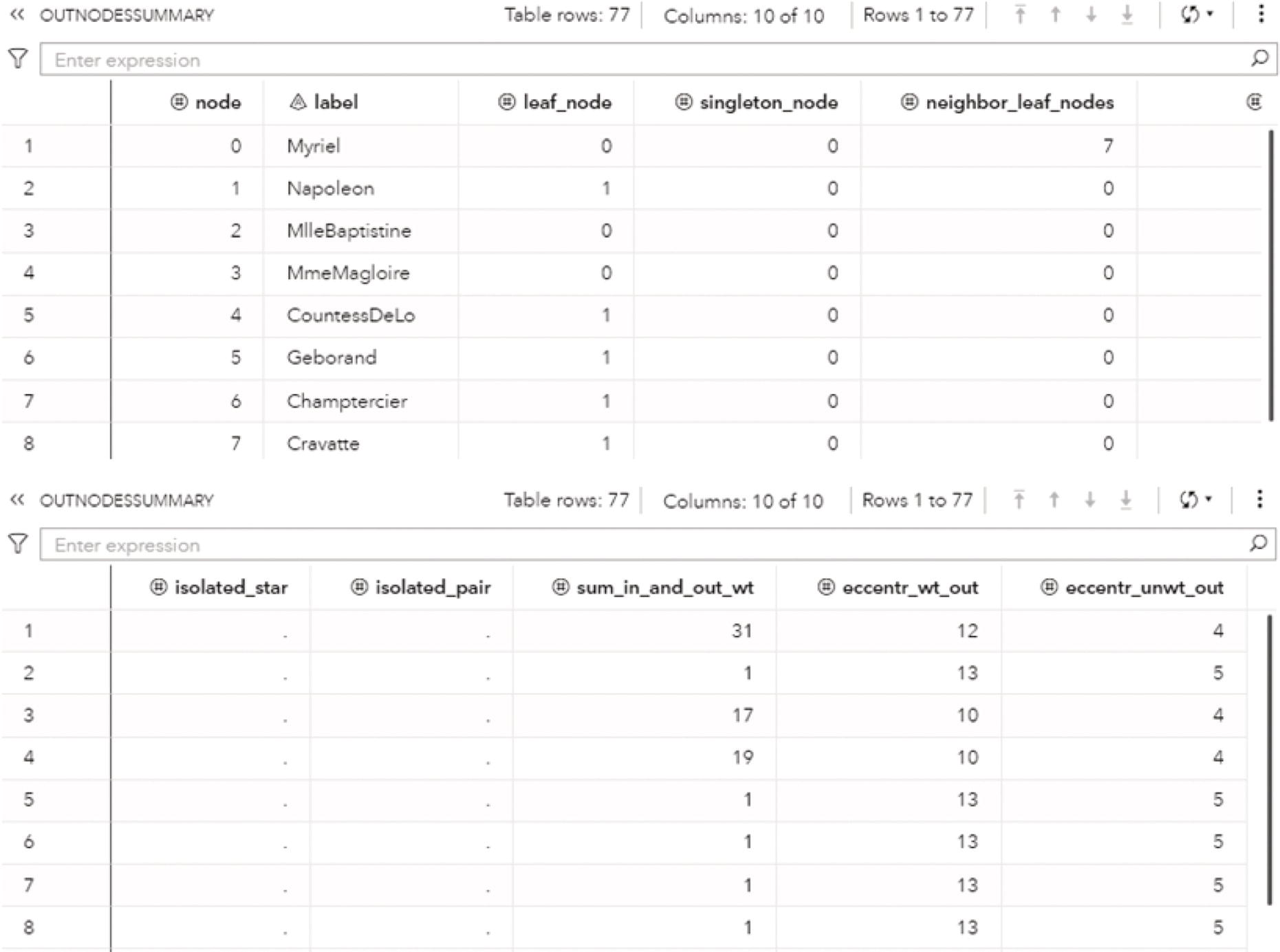
Figure 1.16 Output data for the nodes.
Figure 1.16 shows the OUTNODESSUMMARY output table consisting of information about all the nodes within the network. Each node in the network has an indicator informing if the node is a leaf node and a singleton node. It also shows how many leaf node neighbors the node has, if the node is an isolated star node (connected to two or more nodes where all of them have degree 1), if the node is an isolated pair node (connected to one single node, and that node it is connected only to it), the sum of the link weights from and to the node, the longest weighted shortest path distance from the node, and the longest unweighted shortest path distance from the node.
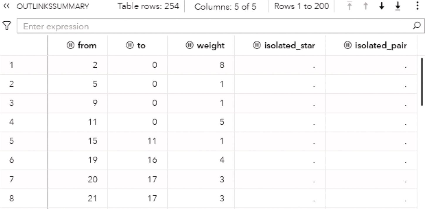
Figure 1.17 Output data for the links.
Figure 1.17 shows the OUTLINKSSUMMARY output table consisting of information about all the links within the network. It shows the original origin and destination nodes, the weight of the link, if the link partakes an isolated star, and if the link partakes an isolated pair.
The Les Misérables network is a small network is very dense, with 77 nodes consisting of one single connected component. That means, all actors can reach out to all other actors throughout a particular path. And that path is not long, with a diameter of 5, which means there four other actors on top between any two. But on average, there are only 2.6 actors in between any pair of actors. There are only 17 nodes with one single connection. Most of the actors play scenes with more than one actor along the movie. On average, they play with 6.6 other actors along the movie.
1.6 Summary
The study of social networks is formally defined as a set of nodes, which consist of network members. Those nodes are connected by different types of relations, which are formally defined as links. Network analysis takes all those connections as the primary building blocks of the social world. Traditional analysis considers individual attributes. Social network analysis considers the attributes of relations in a unique perspective than that adopted by individualist or attribute‐based social science. Traditional methods of data analysis usually consider individual attributes from all observations. What is the average characteristic from a particular population of companies, employees, customers, or markets? Beyond individual attributes, social network analysis considers all information about the relationships (links) among the network members (nodes). In fact, the information about the relations among the individuals within a social network is usually more relevant than the individual attributes of the members of the network. Ultimately, the relations between the individuals within a network can reveal more hidden information about the network members than their individual attributes. This is the basic difference between data analysis and social network analysis.
Graphs can reveal valuable information about social interactions, and therefore, characteristics of communities, groups of people, or even individuals. Graph algorithms can also be used to compute network measures that identify roles and the importance of the network members. There is a wide range of network measures that can be used to describe the importance of nodes and links. Graph algorithms can also detect and identify groups of members in the network based on their relations, whether considering the frequency, the strength, or any combination of relations attributes.
Network analysis is frequently used to better understand customers behavior, highlight influencers in networks, avoid churn, diffuse products, detect fraud, and search for anomalies, among many other applications. Network optimization includes algorithms to solve multiple practical real‐world problems.
Connectors are essential roles within networks. They may know lots of people, many times the number of people the average person knows. They also know essential facts about people. The impact of connectors to business is obvious.
With its origins in social science, there is a long history of network analysis studies to evaluate how people relate to each other and how these relations shape not just how groups of people are created, but also how individuals behave in those groups.
A mathematical formalism is used to describe the network in terms of a graph, and then builds up a set of algorithms to analyze the graph, compute centrality metrics, identify subgraphs, and search for optimal solutions in optimization problems.
One of the most important concepts in network analysis is the small world idea. The concept implies that the world is small because there are a few nodes separating any pair of nodes. In social networks, it means that a person can reach out to any other person in the world by contacting a fixed number of persons in the path. The small world concept is assigned to the concept of six degrees of separation. It states that there is an average number of people (or nodes) in the world (or the network) separating any two persons. This number changes according to the network analyzed.
The following chapters will describe in great details how to identify subgraphs from main network, how to compute network centralities to describe nodes and links, and how to solve multiple optimization problems that can be represented as a network.
All examples presented in this book use SAS procedures in Viya, a multi distributed in‐memory engine. Two procedures are explored. First is the NETWORK procedure, which covers all the subgraphs algorithms shown in Chapter 2 and all the centrality metrics algorithms shown in Chapter 3. Second is the OPTNETWORK procedure, which covers all the optimization algorithms shown in Chapter 4. Chapter 5 presents some case studies to better exemplify how valuable network analysis and network optimization are.