
8
Run-In
8.1. Run-in principle
A particular type of burn-in is known as the run-in. This concept was well-known several decades ago, notably for automobiles. In the past, the purchase of a new car was accompanied by a run-in stage: longer or shorter, not too rapid, not too high in rpms, daily check-up of levels, etc.
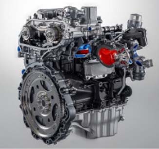
Figure 8.1. Run-in of a car engine. For a color version of this figure, see www.iste.co.uk/bayle/maturity1.zip
First, let us recall what the run-in of a new car entailed. It covered a period of time between the purchase and the first few hundred kilometers traveled, say up to 1,000 km on the counter. The idea was to drive with almost excessive caution, allowing all of the parts and gears to properly interconnect and to erase all machining traces. Conversely, being impatient and pushing the gas pedal to the floor could generate even more friction between the parts, distorting them and increasing oil consumption and, consequently, the number of failures.
On the contrary, a failure is not always defined as the cessation of a function of a component, or its destruction. Indeed, it can also be about no longer reaching a certain level of performance. This is particularly the case with components that have a “reference” function, for example a voltage regulator (electrical voltage), an oscillator (frequency), etc.
These components generally provide a physical quantity with a certain level of precision guaranteed by the manufacturer. However, this level of precision is not always sufficient to meet the requirements of a product specification. Moreover, component performance most often degrades over time and as a result of the temperatures that it is exposed to.
As an illustration, consider the example of a logarithmic drift of equation:
with a = 1.1 and b = -2.4.
This is illustrated in Figure 8.2.
It can be seen that the drift of the component performance almost reaches a value of 5.2 at time = 1,000 hours. Assume that the required specification is 3. As such, this component is not suitable for guaranteeing the specification, although the manufacturer guarantees the best performance.
The idea is then to submit the component to a test, referred to as a stabilization test, at the equipment manufacturer before delivering it to the system manufacturer. Indeed, when calculating the slope of this drift, namely the drift rate in time, it is obvious that it decreases, being inversely proportional with time. In other terms, the component drifts a lot at the beginning and less and less later on. Hence, if the component is submitted to a sufficiently long test at the equipment manufacturer, the resulting component has a drift at the system that meets the demand of the specification.
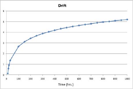
Figure 8.2. Example of concave degradation
Assume that the component is subjected to a test (referred to as stabilization test) of 100 hours. Based on the previous example, Figure 8.3 is obtained.
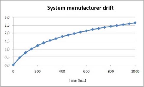
Figure 8.3. Drift after 100 hours stabilization
The specification requiring a maximal drift of 3 after 1,000 hours is then met since it is reached ~2.7 after 1,000 hours.
NOTE.–
To obtain this curve, the drift at 100 hours was subtracted from the drifts obtained for times exceeding 100 hours.
8.2. Stabilization
However, the problem is not that simple for three key reasons:
- – The drift performance is achieved for a period of time equal to the product’s duration of service, which is generally specified in years, or even in dozens of years. A long stabilization time would therefore be needed, which is incompatible with the industrial constraints of the equipment manufacturer.
In order to avoid this problem, with drift generally being greater the higher the temperature of the component, the test at the equipment manufacturer can be conducted at a temperature that exceeds that which the component is subjected to during operation. The virtual acceleration of time makes it possible to have an acceptable stabilization time. The disadvantage of this method is that an acceleration law must be estimated. This can only be done using tests at various temperatures (at least two).
- – The parameters of the drift law (a and b in the previous example) can be very scattered from one component to another. This has two major consequences:
- - the stabilization time cannot be unique and therefore common to all of the components;
- - in certain cases, the stabilization time can be very long and therefore incompatible with the industrial constraints due to a too low drift speed. In this case, it is recommended to preserve the maximal authorized stabilization time and reject the component if this time is exceeded, in order to obtain the expected drift.
- – The drift of the component cannot always be modeled with the drift law valid for the other components. In this case, the component is also rejected.
8.2.1. Proposed principle
The fact that the temperature used during the stabilization stage is higher than the temperature the product will be subjected to during use creates a problem; this is because the Arrhenius law is only valid for a constant temperature. To solve this issue, let us enter the world of Mr. Sedyakin. The principle he proposed for a survival function is also applicable to degradation. Assume the degradation can be written as follows:
Assume the AFT (AF = acceleration factor) model can be used. The degradation can be written in the following forms:
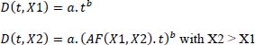
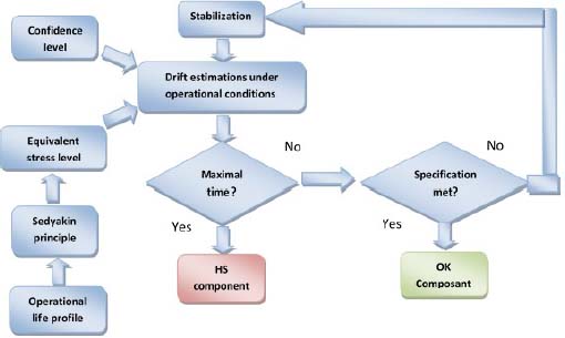
Figure 8.4. Run-in principle. For a color version of this figure, see www.iste.co.uk/bayle/maturity1.zip
Resuming the previous example, Figure 8.5 illustrates these equations.
With the formulated problem, the evolution of physical contribution illustrated in Figure 8.6 is applicable.
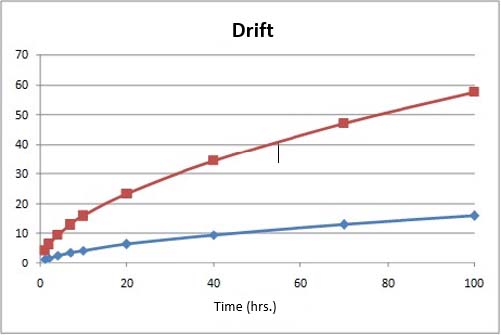
Figure 8.5. Example of degradation with two different levels of physical contributions. For a color version of this figure, see www.iste.co.uk/bayle/maturity1.zip
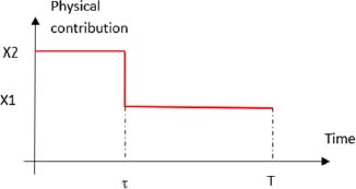
Figure 8.6. Descending level of physical contribution. For a color version of this figure, see www.iste.co.uk/bayle/maturity1.zip
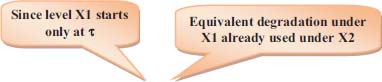
The level of this physical contribution can be written as: X = X1. It≤τ + X2. It>τ. If the component is subjected to a physical contribution of level X2 during a time τ, then level X1, according to Sedyakin’s principle, it can be written as:
For this example, Sedyakin’s principle can be illustrated by Figure 8.7.
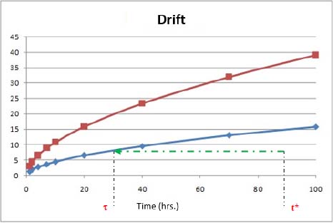
Figure 8.7. Illustration of Sedyakin’s principle for a descending level. For a color version of this figure, see www.iste.co.uk/bayle/maturity1.zip
Equations [8.2] and [8.3] lead to:
or still
8.2.2. Drift acceleration law
The Arrhenius law is generally used to model the effect of temperature (Arrhenius 1889). The insertion of this law into equation [8.1] leads to:
where θ is the temperature of the component during the stabilization test.
AF is the acceleration factor between the accelerated conditions of the test and the reference conditions
NOTE.–
Time acceleration by a physical contribution (in this example, the temperature) can be modeled using the AFT (Acceleration Failure Time) model proposed in Bagdonavicius and Nikulin (2001).
According to the hypothesis of Arrhenius law, this takes the following form:
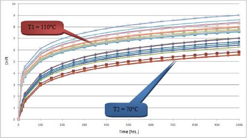
Figure 8.8. Example of the effect of temperature for the drift of a performance. For a color version of this figure, see www.iste.co.uk/bayle/maturity1.zip
Based on equations [8.2] and [8.3], the following can be written for the operational conditions:
To illustrate this, let us resume the example of a logarithmic drift with 10 components for two test temperatures θ1 = 110°C and θ2 = 70°C. Assume that the activation energy is Ea = 0.6 eV.
Figure 8.8 is obtained.
NOTE.–
A small random term was added in the expression of parameter “a” so that there are different trajectories between the components, thus closer to reality.
8.2.3. Choice of the drift model
Several models of drift are possible. The least squares regression line is the method that is typically used. It is important to note that it is the variable that depends linearly on the regression coefficients. For example, a power model is a linear model.
At first glance, several linear models of drift may be suitable. The coefficient of determination R² is often used to verify the quality of the regression. This is an error, for at least three reasons:
- – The same coefficient R² for a case with five drift measures and another case with 50 measures does not necessarily provide the same information on the quality of the chosen model.
- – What is the value of R² starting with which the contemplated model can be considered representative for the data?
- – A model with many parameters has more chances to provide a more precise model in graphical terms.
In order to choose the best-fitted drift model, the use of the Akaike information criterion (AIC) (Akaike 1974) is proposed. The Akaike information criterion makes it possible to penalize models depending on the number of parameters in order to meet the parsimony criterion.
The chosen drift model is the one with the weakest Akaike information criterion. The overview diagram give in Figure 8.9 illustrates the proposed method.
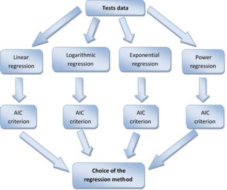
Figure 8.9. Principle of the choice of the drift model
The AIC criterion is defined as follows:
where n is the number of points of measurement; p is the number of parameters of the model; Di is the drift measured at point “i” and ![]() is the drift measured at point “i” and DC is the drift estimated at point “i”.
is the drift measured at point “i” and DC is the drift estimated at point “i”.
8.2.4. Equivalent level of physical contribution
To find the acceleration factor between the accelerated conditions of the test and the operational conditions, the operational life profile – to which the component is subjected – must be known. Most of the time, this is composed of the various operational stages for which the duration and the level of the various physical contributions are known. This division is in fact compulsory because the physical laws of failure (Arrhenius, Coffin–Manson, etc.) are only valid for constant levels. The division into various stages of the life profile makes it possible to apply these physical laws of failure.
It is important to be able to estimate the acceleration factor between the conditions of the stabilization test and the operational conditions for various physical contributions. Sedyakin’s principle (SED 1966; Bayle 2019), more commonly referred to as “cumulative damage”, is used for this purpose, in order to obtain an equivalent constant level of physical contribution in terms of reliability.
For the temperature case, which represents the majority of cases, this leads to:
When the thermal time constant of the product is low compared to the duration of the stages of life profile, the temperature can be considered constant during the stage. According to this hypothesis, the previous equation is written as:
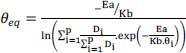
where p is the number of stages of the considered life profile, Di is the duration of stage “i” and θi is the temperature of stage “i”.
Consider the example of a life profile involving 5 stages, as defined in Table 8.1.
Table 8.1. Example of calculation of equivalent temperature
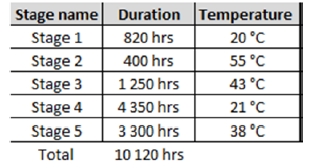
In this example, an equivalent temperature of ~ 34.3°C is obtained.
8.3. Expression of the corresponding degradation
Consequently, the degradation can be written as:
PROOF.–
It can be written that:
Or still, according to equation [8.4]
Or still, according to AFT model
End
Considering a degradation with a power law of parameters a and b, the following relation results:
Consider the following example:
- – a = 2
- – b = 0.56
- – Tm = 10 000
- – AF = 24.7
- – τ = 299
Figure 8.10 is obtained.
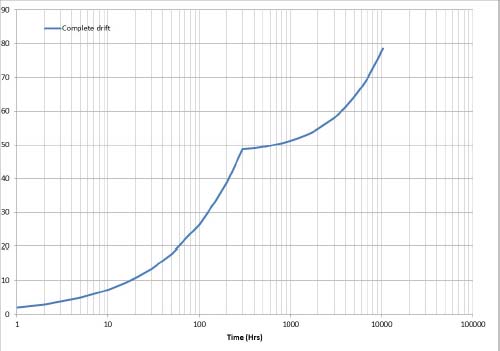
Figure 8.10. Power law drift with temperature change. For a color version of this figure, see www.iste.co.uk/bayle/maturity1.zip
8.4. Optimization of the stabilization time
Considering the previous example, there is a degradation, starting with time τ, of 48.653. If the specified objective is 30, this stabilization time is not appropriate. The value of the optimum stabilization time Dsta required for the operational drift to be lower than or equal to the specified maximal drift D_Obj should be determined.
Therefore:
where Tm is the duration for putting products into service; Xopl is the operational level of the physical contribution of interest and Xacc is the accelerated level of the physical contribution during the stabilization stage.
Equations [8.1] and [8.7] lead to:
Due to the concavity of degradation, 0 < b < 1 and this equation has no analytical solutions. However, the stabilization time can be estimated using numerical methods. The objective is now to find the value of the stabilization time Dsta that minimizes the equation:
Resuming the previous example leads to Figure 8.11.
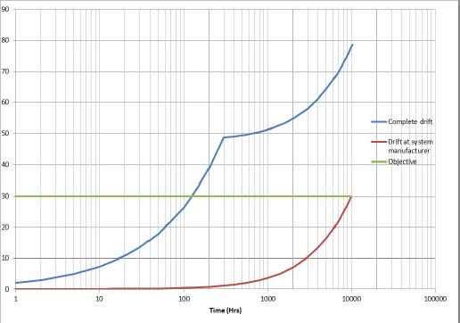
Figure 8.11. Power law drift with change of temperature with optimum stabilization time. For a color version of this figure, see www.iste.co.uk/bayle/maturity1.zip
The result is a minimum stabilization time of 299 hours to maintain the objective of maximal degradation of 20 under operational conditions.
8.5. Estimation of a prediction interval of the degradation
The linear regression theory is used here, and in particular the prediction interval. Indeed, in order to guarantee the preservation of frequency drift during operation with minimal risk, instead of the estimated value of drift, the higher bound of the prediction interval is taken into consideration.
I.e.:
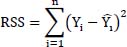
- – RSS (the residual sum of squares) measures the part of the Y variation unexplained by X, defined by:
- – ESS (the explained sum of squares) measures the part of the Y variation explained by the model (by a variation of X), defined by:
The lower and upper bounds of the prediction interval (Rakotomalala 2018) at the confidence level CL are given by:
where n is the number of points of measurement; St-1 is the quantile of Student’s law and t is the instant at which the value of the frequency drift is projected.
Resuming the previous example, Figure 8.12 is obtained.
It is clear that in order to estimate the minimal stabilization time, the upper bound of degradation must be taken into account.
8.5.1. Principle of the stabilization method
The principle of stabilization must meet several constraints, notably it must:
- – guarantee a frequency drift below 1.5 Hz when the equipment is put into operation;
- – have a stabilization duration that does not lead to excessively long test times.
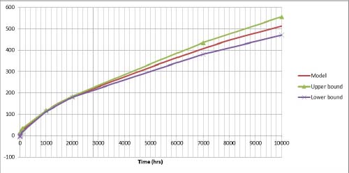
Figure 8.12. Illustration of the prediction interval of a linear regression
The principle relies on a methodology involving two distinct parts as follows, and illustrated by the following figure:
- – A first series of tests allowing an estimation of the acceleration law of frequency drift. These tests were conducted on a sample of specific CDXO.
- – For each CDXO delivered, a specific stabilization criterion had to be set.
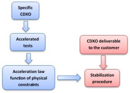
This part presents the modeling results obtained during the accelerated tests conducted on CDXO with the proposed method.
It is important to recall that the stabilization of CDXO to guarantee the preservation of the frequency drift specification involves two stages:
- – A stage of estimation of the acceleration law in temperature and voltage conducted on a sample of dedicated CDXO.
- – An optimization stage of the stabilization time to guarantee the preservation of the specification, which is specific to each CDXO delivered to the customer.
The parameters of the law of temperature drift are specific to each CDXO. Hence, in order to guarantee the preservation of the frequency drift with respect to the specification, it is necessary to optimize the stabilization time of each CDXO individually.