
6
Aggravated Tests
There are many articles and books that offer very precise details of aggravated tests; this is beyond the scope of this chapter. Although a concise description of these tests is provided here, the fundamental aim of this chapter is to explore how these tests relate to product maturity.
6.1. Definition
In the context of this chapter, aggravated tests can be defined as follows:
Tests that submit the product or some of its constituent elements to (climatic, electrical, mechanical) constraints that are progressively increased to values significantly higher than those specified, within the product operation and/or destruction limits.
According to the manufacturers, the above strict definition of aggravated tests does not cover all these practices, particularly in terms of scale of application (the product), application technique (no bias on the value of constraints seen by the product) and even final purpose of the tests.
6.2. Objectives of aggravated tests
There are numerous articles, documents, presentations, etc. on aggravated tests, which include the following points on the use of conducting aggravated tests (McLean 2009):
- – improve product robustness by applying quite serious stresses;
- – highlight the potential weaknesses inherent to product design and to the technologies involved;
- – estimate design margins, as illustrated below;
- – at the card or subassembly level, make a selection based on various technologies or various providers and choose the most robust.

Figure 6.1. Illustration of the principle of aggravated tests. For a color version of this figure, see www.iste.co.uk/bayle/maturity1.zip
The above points are evidently correct and not to be questioned. However, the main objective of aggravated tests is to participate in building product maturity. Estimating the operational limits of the product (and deducing robustness margins), eliminating design weaknesses, etc. are actually means of contributing to building product maturity.
Indeed, identifying design failures and then correcting them will notably improve product reliability by suppressing the reliability increase stage observed in the first operational years of the product, reducing potential aging failures during or by the end of product operation. In other terms, aggravated tests contribute significantly to rendering the operational reliability of the product as constant as possible. Moreover, the resulting robustness margins will also reduce the influence of accidental overloads (catastrophic failures) that are generally present during product operation. This will generally have a non-negligible influence on the observed reliability level, as illustrated in Figure 6.2 below.

Figure 6.2. Influence of aggravated tests on product reliability
6.3. Principles of aggravated tests
The principles of aggravated tests are:
- – to subject the product to various environmental stresses by progressively increasing the levels step by step until the occurrence of a failure;
- – to conduct a root cause analyses for each failure in order to identify whether it is a design defect/failure due to:
- - a design problem,
- - a technological limitation;
- – to decide whether or not corrective action is needed;
- – to reiterate the process of elimination of these weaknesses until design margins that are considered sufficient are obtained.
The “guiding principle” of an aggravated test is not a willingness to “comply” with the requirements of a specification. Its objective is not the verification of technical performance, nor an estimation of service life. The “guiding principle” of an aggravated test is to bring a product to the limit of its capacities, or even to break down, by subjecting it to “what is needed, where it is needed, when it is needed”.
In order to choose the strategy that best fits the manufacturing context of interest, two essential questions must be addressed, namely:
- – Is an aggravated test necessary?
- – If so, what is the most relevant type of test?
In order to answer these questions, all the constraints imposed on the equipment manufacturer must be analyzed.

Figure 6.3. Examples of extrinsic decision criteria for conducting aggravated tests. For a color version of this figure, see www.iste.co.uk/bayle/maturity1.zip
There are two types of aspects guiding the choice of the method:
- Constraints extrinsic to the equipment manufacturer:
- - recommended or even imposed by the system manufacturer;
- - a strict life profile in terms of level of physical contributions. In this case, we can consider that the verification of the proper design and the estimation of design margins are major elements;
- - the context of a highly competitive market, in which the other manufacturers systematically conduct this type of test;
- - very important dependability specifications (critical dreaded events, carrier availability);
- - a large number of products to be delivered. Indeed, as already noted, this type of test aims to eliminate potential design weaknesses. It is known that this type of failure is very often reflected in premature aging that is observed throughout the batch of delivered products. The design modification will therefore have a significant financial impact;
- - very important brand image, guaranteeing the sales of other types of products. Failures observed during operation involve a risk of significant damage to the brand image of the equipment manufacturer.
Figure 6.3 gives the paths of extrinsic decision criteria, which can be adapted as needed. In Figure 6.3, the given criteria can be interpreted as follows:
- – aggravated tests are recommended by the system manufacturer. Indeed, when the latter has a reference product for which this type of test is recommended, it would be difficult not to follow this recommendation;
- – if competition is strong, then reliability (or quality) of the equipment should be maximal and aggravated tests could contribute to fulfilling this need;
- – if the number of products is significant, then the investment required for the aggravated tests will be returned more quickly (and if the product is small, several can be placed in the equipment being used, reducing the time required to conduct the tests);
- – if reliability objectives are high, then aggravated tests are a way of addressing this need by systematically detecting failures and methodically repairing them.
- Constraints intrinsic to the equipment manufacturer:
- - a strategy of conducting tests that are recommended or even imposed by the company;
- - a large variety of such products that are specific to the equipment manufacturer;
- - the company’s brand image;
- - an equipment manufacturer having a “product policy”, meaning operational blocks that are introduced in all the types of products designed by the equipment manufacturer. In case of a design failure on an operational block, all the products designed will feature this failure, with disastrous results;
- - the impact of such tests on the cost of products. Indeed, in certain domains, the cost of such tests may have a significant impact on the final cost of the product and may potentially lead to the loss of important markets;
- - the type of manufacturing domain (aeronautics, automotive, domestic appliances, etc.). This question is not applicable to certain industrial domains, in which aggravated tests must be conducted (e.g. the space industry, which does not tolerate the slightest error).
Figure 6.4 gives the paths of intrinsic decision criteria, which can be adapted as needed.
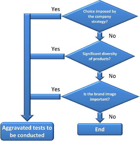
Figure 6.4. Examples of intrinsic decision criteria for conducting aggravated tests. For a color version of this figure, see www.iste.co.uk/bayle/maturity1.zip
Although in certain cases it may be possible to use other aggravated test methods, the recommended method is HALT/HASS (McLean 2009), which is the focus of the next section.
6.3.1. Choice of physical constraints
All previously presented advantages of aggravated tests are not real unless the product is correctly stressed. The choice of physical contributions is therefore essential. Several studies were conducted (IES 1984) on this subject, and their results can be summarized in Figure 6.5 (below).

Figure 6.5. Comparison of the influence of physical contributions for aggravated tests. For a color version of this figure, see www.iste.co.uk/bayle/maturity1.zip
As it is impossible to simultaneously generate constant temperature and have thermal cycling, the dominant condition is kept, namely, the thermal cycling. In fact, the most important physical contributions (thermal cycling, vibration and power cut) were grouped in a single machine, greatly simplifying these tests, particularly in terms of time and costs.
6.3.2. Principle of HALT
In order to find the operational limits of a product, the approach illustrated in Figure 6.6 is used.
Here, the technological limit is identified as being the maximal values guaranteed by the manufacturer of the components. For example, for a component that is guaranteed up to +85°C, the technological limit of the product will be reached when the temperature level of the aggravated test exceeds this value, even if the product is still fully operational.
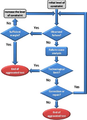
Figure 6.6. Principle of HALT tests. For a color version of this figure, see www.iste.co.uk/bayle/maturity1.zip
HALT testing involves the following process:
- – finding the low-temperature operational limit (LTOL). The starting point is the ambient temperature, which is then decreased in steps of generally 10°C for 10 min. If the product is operational, the temperature is further decreased by 10°C until an operational failure occurs. This can be illustrated by Figure 6.7 (below);
- – finding the high-temperature operational limit (UTOL). The starting point is the ambient temperature, which is then increased in steps of generally 10°C for 10 min. If the product is operational, the temperature is further increased by 10°C until an operational failure occurs. This can be illustrated by Figure 6.8 (below).

Figure 6.7. Finding the low temperature operational limit
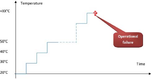
Figure 6.8. Finding the high temperature operational limit
NOTE.– It is not surprising that destructive low-temperature limits are rarely reached by electronic materials. They are indeed more sensitive to high operational temperatures than to low operational temperatures.
- – Finding the vibration operational limit (UVOL). The starting point is the vibration in Grms, which is increased in steps of generally 5 Grms for 10 min. If the product is operational, the vibration level is further increased by 5 Grms until an operational failure occurs. This can be illustrated by Figure 6.9 (below).
It is important to note that vibrations take place along 6 degrees of freedom (one translation and one rotation per axis) and that the product being tested is at the ambient temperature. The duration of one step is of minimum 10 minutes, but it may take longer to conduct the required tests. Vibrations generally range between 2 Hz and 5 kHz.

Figure 6.9. Finding the vibration operational limit
- – Finding the operational limits by a combination of vibrations and thermal cycling.
A combination of constraints, such as vibrations and thermal stresses, can be used to reveal latent weaknesses of the equipment, which do not occur under a single constraint (e.g. temperature only or vibration only).
NOTE.– Moreover, during each of these steps, the package is monitored (controlling the operational tolerance drift and recording the constraints and their responses at the card level) so that defects due to temperature change are detected.
- – Unless it is checked by other tests, it is useful to check the cold start of the equipment at various steps. This is an additional test, which involves checking the start of equipment under stabilized low temperatures, in order to determine its limit. It is distinct from ON/OFF cycles, as the latter are conducted on an initially operating equipment, whose components have a higher temperature than the environment, especially if it is very dissipative.
Figure 6.10 illustrates this process.

Figure 6.10. Finding the operational limit for combined thermal cycling/vibration constraints. For a color version of this figure, see www.iste.co.uk/bayle/maturity1.zip
NOTE.– The above example of combined cycle does not take into account thermal inertias, which can be generated by a collapse. The thermal profiles (temperature slope/step duration) must be corrected to fit the constraints. The time needed to initialize the equipment and the monitoring software must also be taken into account.
- – The application tolerances of the acceptable constraints are generally of ±3dB in vibration about the rated profile and ±2°C in thermal cycling.
6.3.3. Specific or additional constraints
The nature of the physical contributions or specific stresses to be applied is suited to the tested equipment. It is therefore difficult to formulate a generic list. Moreover, when non-electronic equipment is involved, the constraints and the stresses to be applied through a testing process are defined case by case.
For electronic materials, the following specific tests can be taken into consideration during a testing process, if their relevance is approved during the stage of constraint selection:
- – power cycle;
- – cycle of various supply voltages combined with previous sequences;
- – finding the limit alternative voltages as well as the limit frequencies;
- – finding the maximum direct supply voltages.
For mechanical materials, the following constraints can be taken into consideration:
- – continuous increase of mechanical load;
- – increase of speed or frequency of mechanical loads;
- – incremental increase of the load acceleration.
The above list is just an example, and is not exhaustive. Its purpose is to show the diversity of constraints that can be implemented during an aggravated testing process. The preliminary stage of analysis and determination of constraints and constraints to be implemented during a process is therefore very important.
6.3.4. Number of required samples
According to the referenced literature (McLean 2009), due to the dispersion of results according to the tested products and the representativeness, it is recommended to use four products per robustness test. However, for highly expensive products and provided that the dispersion of the various operational limits observed is very weak, a single sample may be used per type of test.
6.3.5. Operational test, diagnosis and identification of weaknesses
It should be possible to stimulate and test the product throughout the testing process so that reversible malfunctions and breakdowns are detected. Test coverage should be sufficient, and it should be possible to observe the evolution of temperature performances, if the function depends on it. It is highly recommended that we conduct a preliminary analysis of the range of temperatures specified for all the components and their expected performances according to the datasheet provided by the manufacturer. This will help in identifying the operational chains that will probably be impacted first during temperature margin tests and to make sure that the test covers these functions.
6.3.6. Monitoring specification
The set of parameters to be measured and therefore to be monitored during the various testing sequences should be defined before the HALT tests. Indeed, it may prove necessary to adapt certain testing methods and even the equipment itself in order to have or allow a proper monitoring.
It is important to differentiate between:
- – Operational monitoring, which is the monitoring of product functionalities. Operational monitoring of the equipment is required for deciding on the proper operation of the electronics at any moment of the aggravated test. Defects can be evidenced by monitoring analysis, and it is important to know which operational constraint generated which defect. This makes it possible to identify the electronic functions that failed under constraint and to rapidly define the failing component.
- – Recording the stresses perceived by the equipment: a proper instrumentation is a must for the analysis of resulting defects, notably the identification of defects due to reaching the technological limits.
For each test monitoring sequence, the following must be defined:
- – parameters to be monitored;
- – operational constraints to be applied;
- – functions covered by the tests;
- – frequency of tests (every 30 seconds, etc.);
- – type of test (intrusive, such as the injection of breakdowns, specific or mobile probe);
- – number of defects based on which a breakdown is confirmed;
- – inhibition conditions;
- – behavior of the associated product.
6.3.7. Instrumentation
In order to properly grasp the levels of involved constraints, the product subjected to aggravated tests must be instrumented. This instrumentation (thermocouples, accelerometers, constraint meters, etc.) can also be used to instantaneously measure the response of the product to constraints. The implementation of this instrumentation is defined based on risk analyses and focuses on the most sensitive components, therefore, the electronic components. For example, on electronic cards, accelerometers are placed on vibration-sensitive components in order to check their maximal displacements during testing.
Vibrational and thermal profiles must be measured at points where it is possible to reconcile the operational defect of the equipment and the applied constraints, or even to estimate the card damage. These profiles must be recorded by accelerometers and temperature probes whose location guarantees a proper application of the constraint during burn-in, in view of proper traceability.
6.3.8. Root cause analysis, corrective actions and breakdown management
Root cause analysis is an integral part of the aggravated testing process. It offers the certainty that the malfunction is related to the test during which the defect appeared, and not to previous stresses, or that the defect is not related to anything else (damage related to the rig, manufacturing defect, manipulation error, etc.).
The root cause analysis process must be documented with the failure mode, the exact cause of failure or its suspected cause, in case of uncertainty.
Failure analysis involves two significant stages:
- 1) electrical diagnosis, which confirms and characterizes the electric defect and guides the physical analysis;
- 2) physical analysis, which identifies the defect location and determines its root cause.
By identifying the root cause of the failure, it is possible to devise appropriate corrective actions, depending on the margin being found. Depending on the type of weakness detected during the tests and characterized by the analysis, corrective actions may involve:
- – changing the reference of a component;
- – modifying the location of a component;
- – locally reinforcing a component (collage, underfilling);
- – reviewing the mechanical design of the card (thermal drain, mechanical maintenance).
A test is considered successful if it highlights as many potential defects of the material as possible. It is important to consolidate all this information, upstream and downstream of the operation, in order to optimize the initially chosen aggravated test. This requires implementing a product to collect information related to failures. This product must be related to the failure modes observed:
- – during the aggravated test;
- – after the aggravated test (material acceptance, client refusal).
Therefore, the information collection may be composed of:
- – the testing reports for each material;
- – the results of the aggravated tests of the materials;
- – the return of experience (RETEX).
A copy of the testing report is attached to each unit subjected to an aggravated test. It contains at least the following elements:
- – identification of the material (designation, reference, serial number);
- – the test result.
For each breakdown observed, the following elements should also be mentioned in the report:
- – the type of cycle during which the defect occurred (e.g. vibration or thermal cycle);
- – the findings;
- – the defective components;
- – corrective actions;
- – the number and type of cycles throughout the stages;
- – the date.
It is important to have a follow-up of corrective actions. Hence, a file containing the results of aggravated tests should be edited regularly. It indicates the number of objects subjected to aggravated tests for each type of material and mentions the causes of breakdowns as well as the actions taken in order to repair the material. In principle, this report should be drawn up by the quality assurance in manufacturing department.
Finally, a report of the equipment returns must also be edited regularly. For each piece of equipment returned, the report should indicate:
- – the conditions under which the failure occurred;
- – the operating mode of the equipment;
- – the age of the equipment;
- – the operating hours, the number of kilometers, etc.;
- – the serial number of the equipment;
- – the place and date of the incident;
- – the conditions of the return to the workshop (transportation mode, operations conducted, etc.);
- – the examination result;
- – the cause of failure (if confirmed);
- – the failed component(s), if applicable.
These elements can be used in the intervention on design, manufacturing operations or on the effectiveness of aggravated tests.
6.3.8.1. Failure analyses
The objective of failure analysis is to determine the failure mechanism and the root cause of the defect. These causes can be grouped into the following categories:
- – manufacturing defect of the component, printed circuit, etc.;
- – damage induced by the manufacturing cycle, handling errors;
- – damage induced by the rig or by the testing means (electrical constraint);
- – design defect.
The interest of the analysis is thus to act at the earliest possible instant on the origin of the failure and to conduct the corrective actions (manufacturing processes, burn-in operations) to prevent failure recurrence. It also reinforces the effectiveness of the aggravated tests.
Failure analysis involves two large stages:
- – Electrical diagnosis: this is used to confirm and characterize the electrical defect and thus guide the physical analysis.
- – Physical analysis: this is most often destructive and can be used to locate the defect and determine its root cause.
Failure analyses can also be used to evaluate the effectiveness of aggravated tests by determining the way in which the applied constraints led to revealing the defect. Failure analysis can be used to distinguish the real from “false” defects. “False” defects are those that can be attributed to a component during the card or equipment diagnosis, though they are not directly due to the component (or another element).
As an illustration, the typical average cost of such an analysis ranges between approximately 4,000 € and 10,000 € in a specialized laboratory. The failure analysis cost depends on:
- – the complexity of the component (test and electrical diagnosis);
- – the reproducibility of the defect (intermittent breakdown);
- – the type of physical defect (ease in locating and identifying the defect).
An example of observed failure/breakdown and corrective action: during the vibration aggravated tests, we observe a failure of component pins. The adequacy of the component robustness is then to be determined according to the operational demands (depending on the margins to be reached).
6.4. Robustness
6.4.1. Estimation of robustness margins
This chapter explains how to determine the operational margins of a product by aggravated tests. In fact, many documents recommend the estimation of the robustness margins of a product but they do not explain how to check that they are sufficient. This chapter proposes a method to meet this objective.
Margins are determined once the operational limit is estimated through HALT tests. The margin is then defined as follows:
For example, at a high temperature, a product can be specified at 85°C and have an operational limit at 108°C. The resulting margin is therefore 108 – 85 = 23°C. This notion of the margin is obviously applicable to all the physical contributions implemented in the aggravated test.

Figure 6.11. Links between margins and aggravated tests. For a color version of this figure, see www.iste.co.uk/bayle/maturity1.zip
6.4.2. Sufficient margins
The fact that a design should be reviewed when the margins are insufficient is often mentioned. This requires a definition of what a “sufficient margin” means. Moreover, this may depend on the manufacturing constraints inherent to the product concerned, and what is acceptable for one application may not necessarily be so for another.
Hence the use of the “resistance/constraint” method, well known in mechanics, is proposed here. Here, the constraint is the specification required by the system manufacturer, while the resistance is the operational limit estimated during the HALT test.
Resistance R and constraint C are considered as two random variables following a normal distribution, which leads to:
where
μc is the level of the physical contribution of interest given in the specification;
σc is obviously zero;
μr is the average of operational limits of products having undergone a HALT test;
σc is the standard deviation of the operational limits of products having undergone a HALT test.
It is possible to estimate failure probability, meaning the probability that the resistance R is weaker than the constraint C, leading to a product failure. The margin is then considered as sufficient when the probability P(R < C) < Ptarget, where Ptarget is the objective probability depending on the application. The difficulty is then in estimating the target probability.
Given the previous hypotheses, it can be shown that the probability of having a failure (in fact, that the resistance is weaker than the constraint) is given by:

where ϕ is the distribution function of the standard normal distribution. Since σc is zero, this finally leads to:
The target probability for the two types of manufacturing applications should therefore be estimated.
6.4.2.1. The reliability objective is the probability to fulfill the mission
Considering all the elements involved in the calculation of this probability as independent, if “n” is the number of elements, then:
Referring to Chapter 1, this probability can also be written in terms of the type of failures as follows:
where Rj, Rc and Rv are the proper operation probabilities of youth, catastrophic and aging failures, respectively. It is possible to formulate a hypothesis according to which, thanks to burn-in, there will be no youth failures or, more reasonably, their influence will be negligible or Rj(t)~ 1. Based on predictive reliability methods, an estimation of the proper operation probability of catastrophic failures can also be made.
Finally, the analysis of components with limited service life, which was developed in this chapter, can be used to give an estimation of the proper operation probability of the aging failures. Hence, based on all these estimations, it is possible to deduce a value of the probability Ptarget. To illustrate the proposed approach, consider the following example:
Assume that a product is specified at a maximal temperature, of +85°C. It can be readily deduced that:
- – μc = 85°C;
- – σc = 0.
Assume that the HALT test provided a temperature operational limit of +90°C, or μr = 90°C (the failure during the HALT test was observed at Ta = 95°C). If several products were subjected to the HALT test, the standard deviation of the temperature operational limit can be estimated. If a single product was subjected to the HALT test, then a standard deviation of 4°C can be considered, according to (McLean 2009). Let us formulate this last hypothesis so that σr = 4°C.
The failure probability given by equation [6.2] can then be calculated, Pdef ~ 8.8 10-5.
Let us assume that the objective of product reliability at the end of mission of duration Tm = 10 years is Rp(Tm) = 95% and that the catastrophic failure rate is λc = 2.21 10-8.
The proper operation probability of catastrophic failures is therefore at the end of mission Rc(Tm) = 98.083%. Consequently, if there are no youth failures, no aging failures, the probability Ptarget must be:
Or numerically: Rtarget ≥ 96.857%. The failure probability was estimated at 8.8 10-5 or a proper operation probability of 99.379%.
The reliability objective is therefore met in this purely virtual example.
6.4.2.2. The reliability objective is an MTBF
For this type of application, reasoning directly in terms of proper operation is no longer applicable, since the specified reliability objective is an MTBF. For this type of application, the maintenance is generally corrective (the failed component is instantaneously replaced by a new one). The notion of rate of occurrence of failure (Rocof) must be introduced, which is generally a time-dependent quantity. However, according to the hypothesis of catastrophic failures, it is known that Rocof is constant and equal to the failure rate λc of catastrophic failures.
For this type of application, repair times are generally negligible compared to the proper operation time so that MTBF ~ MTTF, and therefore ![]() .
.
Resuming the previous hypotheses, it can be reasonably expected that youth and aging failures are not observed, leaving only catastrophic failures so that:
Therefore, λHALT ≤ λtarget.