
1
Reliability Review
In this book, maturity is defined as the ability of a product to achieve the expected level of reliability from the moment it becomes operational for the end user. A review of what reliability means and a definition of the parameters on which it is based is therefore needed.
1.1. Failure rate
Reliability studies the occurrence of failures in time. These instances of failure are random; hence, they cannot be known in advance. This presents a challenge. To model them, we use the concept of random variable, which will be denoted by T throughout this book.
First, it is important to determine the various types of failures. There are three main categories, namely:
- – “youth failures”, which generally occur very early on in the lifecycle of a product. Youth failures are generally the result of manufacturing defects. Therefore, they concern only a small part of the population. They can be partially eradicated by specific tests, such as burn-in;
- – “catastrophic failures”, which are unexpected, sudden and independent of the time previously elapsed. These types of failures can therefore be observed at any point in the lifecycle of a product. They are generally the result of accidental overloads (heat, mechanical, electrical). They typically do not concern the entire product population and can be reduced by robustness tests, derating rules, etc.;
- – “aging” failures, which are observed across all the products in operation. These failures are generally not observed during the lifecycle of a product, with the exception of specific components with a “limited service life” or premature aging, as a result of poor sizing, a batch of defective components, etc. They affect the entire population and therefore must be absolutely pushed beyond the duration of use of the product. Consequently, design rules (derating rules, worst-case analysis, thermal, mechanical, electrical simulation, etc.), and specific aging tests can be implemented.
We begin by addressing intrinsic reliability. Intrinsic reliability refers to the reliability of a component, a card or a product in the absence of any maintenance. In order to estimate this, and in particular to know the type of failure involved, the most widely used parameter is the (instantaneous) failure rate denoted by λ, which is defined by:
Let us briefly analyze this equation and the following conventions. The term P denotes the “probability” and the symbol “/” stands for “knowing that”. The limit “lim” represents the instantaneous character of the failure rate. Therefore, equation [1.1] can be interpreted as follows:
Probability that the product will fail between “t and t+dt” knowing that it was operational (non-defective) at instant “t”.
To facilitate understanding of the concept of failure rate, the analogy with a human being can be used (Gaudoin and Ledoux 2007). Let us try to estimate the probability that a human being dies between 100 and 101 years of age. This probability is low since the majority of human beings die before they reach 100 years old. Furthermore, let us estimate the probability that a human being dies between 100 and 101 years of age, knowing that they were alive at 100 years old. This probability is high, as human beings do not live long after reaching 100 years of age.
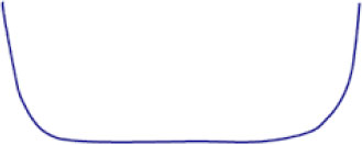
The three failure categories can thus be symbolically represented using the concept of failure rate using the famous bathtub curve, as illustrated in the following figure.
The most commonly used mathematical object for modeling failure rate is the Weibull distribution. According to this hypothesis, the latter is defined by:
where η is a scale factor (generally time-dependent) and represents typical service life, characterized by the fact that the failure rate is ~ 63.2% (1 – exp(-1)), irrespective of the value taken by the parameter β and therefore of the type of failure.
This modeling is interesting for the following three reasons:
- – the mathematical formulation is simple, as it involves a versatile power function (differentiable, integrable, etc.);
- – depending on the parameter β, this function is decreasing (β < 1), constant (β = 1) or increasing (β > 1). In other terms, it can represent the three types of previously defined failures;
- – the parameter β has a physical significance as it represents the aging dynamics of the observed failure mechanism. Indeed, as already noted, failure instants are characterized by randomness (components tested are assumed to be identical). This means that instead of having a single real value, if failures were purely deterministic, we see a constant dispersion of failure instants. In fact, the parameter β is the image of this dispersion, and the greater it is, the less dispersed the instants of failure are. Ultimately, if β was infinite, all the failure instants would be identical, which is obviously never the case in practice.

Figure 1.2. Fall leaves illustrating aging. For a color version of this figure, see www.iste.co.uk/bayle/maturity1.zip
This figure clearly shows that all of the components – in this case, the leaves – are subject to aging, yet not all of them fail at the same time (not all the leaves have fallen at the instant shown).
As an illustration, let us assume a Weibull distribution whose scale factor is η = 1,000 (this value is a purely conventional value and could be quite different without changing the conclusions obtained). Furthermore, let us assume that there are 30 components in a test and failure instants are generated for each of them in a purely virtual manner for two values of β (3 and 10).
The following figures are obtained, with time on the ordinate (horizontal) axis and the number of components on the abscissa (vertical) axis.
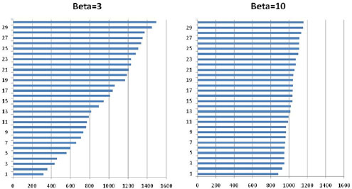
It can be noted that failure instants are more dispersed for β = 3 (on the left) than for β = 10 (on the right). On the other hand, for β = 1, equation [1.2] is written as: ![]() or, more frequently, as:
or, more frequently, as:
This represents the exponential distribution law modeling catastrophic failures. The failure rate for this category of failures is constant, which means that failure instants do not depend on the elapsed time. This specificity of the exponential law is known as the “memoryless property” (it is the only continuous law with this property). Indeed, returning to the analogy with human beings, a catastrophic failure is, for example, a car accident occurring when a driver cuts off another driver. This “failure” does not depend on the distance traveled, but is due solely to the recklessness of another person. This is entirely different from an aging failure, for which the failure instant directly depends on the distance traveled, because this relates to driver fatigue.
It is important to note that the concept of maturity has no qualitative meaning for non-maintained products. Indeed, the objective of reliability is a probability of success; the mission is achieved by the survival function, which for a Weibull distribution is defined as:
This survival function – and this is the case regardless of the law used – is a strictly decreasing function of time. Therefore, the concept of constant reliability is not applicable. For most non-maintained industrial applications, exponential distribution is preferred to Weibull distribution; this is because the reliability objective is a probability of achieving the mission, whose value is obviously high (generally such that R ∈[90% ; 99%].
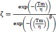
In this case, we can return to an exponential distribution because, for these values of the survival function, it is conservative, with respect to a Weibull distribution, whose shape parameter is greater than 1. Indeed, from a mathematical perspective, the ratio of the two survival functions can be calculated as follows:
with β > 1 and Tm = mission duration.
To obtain a sufficiently high probability of success in the mission (survival function) requires Tm/η ≪ 1. Consequently, β being greater than 1, ![]() . Using an expansion up to the first order of the exponential function leads to:
. Using an expansion up to the first order of the exponential function leads to:

Since Tm/η is greater than ![]() , the numerator is smaller than the denominator and therefore ζ < 1. Hence, the exponential survival function is lower than that of Weibull, which proves that it is conservative.
, the numerator is smaller than the denominator and therefore ζ < 1. Hence, the exponential survival function is lower than that of Weibull, which proves that it is conservative.
Another, more physical way to view this result is to remember that the shape parameter β represents the dispersion of time until failure. The greater β is, the less dispersed the time until failure. Since the Weibull shape parameter is > 1, the corresponding failure instants are less dispersed around the scale parameter η.
Consequently, failures following an exponential distribution with an identical scale parameter occur earlier than those following the Weibull distribution. Therefore, the survival function of the exponential distribution at any instant “t” is weaker than that of the Weibull distribution, which proves the conservative character of this approach.
1.2. Temperature effect
Temperature is systematically involved in component failure mechanisms. The Arrhenius law is generally used in order to model its effect on the reliability of components. Based on an empirical research method, that is, studied through a number of experiments, the Arrhenius law is used to model the variation in the speed of certain chemical reactions under the influence of temperature. With respect to the previously described Weibull law, the following formulation is obtained:
| with | |
| Ea is the activation energy. | |
| Kb is the Boltzmann constant. |
1.3. Effect of maintenance
In most industrial applications, the focus is on the reliability observed on the ground, which must take into account the maintenance actions carried out. Maintenance can take several forms, depending on the level at which it is being performed (components, products, etc.). At the component level, maintenance is generally referred to as “perfect”, also known as “corrective maintenance”, since defective components are replaced with new ones.
At the product level, maintenance may be referred to as “preventive”. This is the case with cars, for example, where engine oil, various filters, etc., are changed on a regular basis without any failures having been observed. More generally, there is “minimal” maintenance at the product level, as replacing the defective component effectively restores the reliability of the product to the level it had before the failure.
Therefore, maintenance has an important effect on product reliability, as illustrated by the following figure.

Figure 1.4. Example of a car that has not been maintained. For a color version of this figure, see www.iste.co.uk/bayle/maturity1.zip
For further details on the effect of maintenance on reliability and its (rather difficult) modeling, the reader is invited to refer to Rigdon and Basu (2000), Gaudoin and Ledoux (2007) and Bayle (2019).
1.4. MTBF
For most industrial applications, the objective of reliability is MTBF. There is much confusion surrounding this acronym; indeed, MTBF may signify:
- – Mean time before failures:
In this case, failure instants were observed on “n” components (or products) assumed to be identical. This is equivalent to MTTF (Mean Time To Failure), as there are no maintenance actions. This can be illustrated by Figure 1.5.
- – Mean time between failures:
This refers to the mean time between two consecutive failures. If there are two failures, this means there was a maintenance action, as illustrated in the following figure.
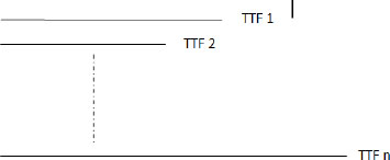
Figure 1.5. MTBF (mean time between failures)
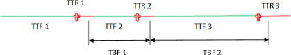
Figure 1.6. MTBF (mean time between failures). For a color version of this figure, see www.iste.co.uk/bayle/maturity1.zip
When there are maintenance actions, the concept of failure rate has no meaning after the first failure. Hence, time between failures (TBF) and time to repair (TTR) are used. MTBF is therefore defined here by:
NOTE.– In practice, the TTR is often very short compared to the TBF; thus, the numerical expression of equation [1.8] can be written as:
Moreover, if the product is mature (no youth or aging failure), then ![]() .
.
According to these hypotheses, equation [1.8] can be written as:
This equation is often found in the literature but is only numerically true under certain hypotheses (exponential distribution), which must be verified.
1.5. Nature of the reliability objective
Product specifications always include a reliability objective. There are two main industrial applications:
- – The first is less common, requiring a probability of success. This probability, which is a function of the product use time, is therefore generally provided after the product becomes operational. The unilateral lower bound of this probability is generally used as the reliability objective. This is due to the fact that it applies to one or several products for which operational failure is to be excluded (e.g. Ariane rockets or certain military weapons).
- – The second covers all other applications (avionics, motor vehicles, rail, etc.) where the mean number of failures is examined. This is the well-known MTBF.