
8
Optimal Execution of Portfolio Transactions with Short-Term Alpha
8.1 INTRODUCTION
In recent years, we have witnessed an increasing use of quantitative modeling tools and data processing infrastructure by high frequency trading firms and automated market makers. They monetize the value of the options written by institutional trade algorithms with every order placement on the market. This creates a challenge for institutional traders. The result for institutions is that trades with poor market timing typically execute too fast and those that have high urgency tend to execute too slowly and sometimes fail to complete. When the market controls the execution schedule, it is seldom to the advantage of the institutional trader.
To cope with this problem, the trader needs to perform three challenging tasks. First, develop an understanding of how urgent a trade is, i.e., when the benefits of speedier execution outweigh the additional impact costs. Second, map this urgency to an optimal execution schedule; and, third, implement the schedule efficiently in the presence of market noise – a stochastic optimization problem. The industry is increasingly working to solve each of these three problems.
Our purpose in this chapter is to address the second task: assign an optimal trade schedule given a view on short-term alpha. To this end, we propose an alternative framework to AC 2000 that is based on more realistic assumptions for market impact and explicitly considers the possibility of a directional bias, or “short-term alpha”.
Our framework addresses the optimal execution of a large portfolio transaction that is split into smaller slices and executed incrementally over time. There are many dimensions to this problem that are potentially important to the institutional trader: liquidity fluctuations, the news stream, order flow imbalances, etc. In response to these variables, traders make decisions including the participation rate, limit price, and other strategy attributes. We limit the scope of the problem by adopting the definition of optimal execution from Almgren and Chriss (2000): optimal execution is the participation rate profile that minimizes the cost or risk-adjusted cost while completing the trade in a given amount of time.
To optimize the risk-adjusted cost, one must first specify a model for market impact. Market impact has been analyzed for different authors as a function of time and trade size. See, for example, Bertismas and Lo (1998), Almgren and Chriss (2000), Almgren et al. (2005), and Obizhaeva and Wang (2006).
Almgren and Chriss' landmark paper derived execution profiles that are optimal if certain simplifying assumptions hold true. These include the hypothesis that the market is driven by an arithmetic Brownian motion overlaid with a stationary market impact process. Impact is proposed to be the linear sum of permanent and temporary components, where the permanent impact depends linearly on the number of traded shares and the temporary impact is a linear function of the trading velocity. It follows that total permanent impact is independent of the trade schedule. The optimal participation rate profile requires trading fastest at the beginning and slowing down as the trade progresses according to a hyperbolic sine function.
This type of front-loaded participation rate profile is widely used by industry participants, yet it is also recognized that it is not always optimal. Some practitioners believe that the practice of front-loading executions bakes in permanent impact early in the trade (Ben Sylvester, personal communication), resulting in higher trading costs on average. A related concern is that liquidity exhaustion or increased signaling risk could also lead to a higher variance in trade results (Hora, 2006), defeating the main purpose of front-loading. In their theory paper, Almgren and Chriss acknowledge that the simplifying assumptions required to find closed-form optimal execution solutions are imperfect. The nonlinearity of temporary impact in the trading velocity has been addressed previously in Almgren (2003) and Almgren et al. (2005); the optimization method has also been adjusted for nonlinear phenomenological models of temporary impact (Loeb, 1983; Lillo et al., 2003). However, most studies share the common assumptions that short-term price formation in nonvolatile markets is driven by an arithmetic Brownian motion and that the effect of trading on price is stationary; i.e., the increment to permanent impact from one interval to the next is independent of time. In addition, the temporary impact is a correction that depends only on the current trading velocity but not on the amount of time that the strategy has been in operation. We find reasons to doubt the assumption of stationary impact. Practitioners find that reversion grows with the amount of time that an algorithm has been engaged; this suggests that temporary impact grows as a function of time. Phenomenological models of market impact consistently produce concave functions for total cost as a function of trade size; this is inconsistent with linear permanent impact.
In previous work (Farmer et al., 2011) (FGLW) showed that it is possible to derive a concave shape for both temporary and permanent impact of a trade that is executed at a uniform participation rate. The basic assumption in this theory is that arbitrageurs are able to detect the existence of an algorithm and temporary impact represents expectations of further activity from this algorithm. The concave shape of market impact follows from two basic equations. The first is an arbitrage equation for traders who observe the amount of time an execution has been in progress. They use the distribution of hidden order sizes to estimate the probability that the hidden order will continue in the near future. The second is the assumption that institutional trades break even on average after reversion. In other words, the price paid to acquire a large position is on average equal to the price of the security after arbitrageurs have determined that the trade is finished. The model explains how temporary impact sets the fair price of the expected future demand or supply from the algorithmic trade. When the trade ends and these expectations fade away, the model predicts how price will revert to a level that incorporates only permanent impact. The shape of the impact function can be derived from knowledge of the hidden order size distribution. If one believes the hidden order size distribution to have a tail exponent of approximately 1.5, the predicted shape of the total impact function is a square root of trade size in agreement with phenomenological models including the Barra model (Torre, 1997). See also, Chan and Lakonishok (1993, 1995), Almgren et al. (2005), Bouchaud et al. (2009), and Moro et al. (2009).
Hidden order arbitrage theory has been extended to varying participation rate profiles by the authors (Criscuolo and Waelbroeck, 2010). They add the assumption that temporary impact depends only on the current trading speed and total number of shares acquired so far in the execution process.
This chapter is organized as follows. In Section 8.2, we use the extended hidden order arbitrage theory to derive the cost functions for two optimal execution problems. In Section 8.3.1, the minimization of trading cost is given a specific directional view on short-term alpha decay. In Section 8.3.2, the minimization of risk-adjusted cost in the absence of short-term alpha is discussed. It is of interest when risk is a consideration but one has no directional bias on the short-term price trends in the stock. In Section 8.4, we will derive numerical solutions in the cases of some relevance to institutional trading desks. In the concluding section, we discuss the implications of our results to the choice of benchmarks used at institutional trading desks to create incentives for traders.
8.2 SHORT-TERM ALPHA DECAY AND HIDDEN ORDER ARBITRAGE THEORY
The alpha coefficient (α) and beta coefficient (β) play an important role in the capital asset pricing model (CAPM). Both constants can be estimated for an individual asset or portfolio using regression analysis for the asset returns versus a benchmark. The excess return of the asset over the risk-free rate follows a linear relation with respect to the market return rm as
where ![]() is the statistical noise with null expectation value. The variance of asset returns introduces idiosyncratic risk, which is minimized by building a balanced portfolio, and systematic risk, for which the investor is compensated through the multiplier beta. The same terminology is used to project future returns: a portfolio manager will assign α to desirable positions based on estimated target prices. It is common to borrow from this terminology in the trade execution arena. The expected market return over the execution horizon is generally assumed to be zero, so the term “short-term alpha” is used by different authors to denote either the expected return of a stock or the expected alpha after beta-adjustment, as given in (8.1). To address the optimal execution problem it is important to know not only the total short-term alpha to the end of the execution horizon but also the manner in which it decays over time. There are four cases of interest:
is the statistical noise with null expectation value. The variance of asset returns introduces idiosyncratic risk, which is minimized by building a balanced portfolio, and systematic risk, for which the investor is compensated through the multiplier beta. The same terminology is used to project future returns: a portfolio manager will assign α to desirable positions based on estimated target prices. It is common to borrow from this terminology in the trade execution arena. The expected market return over the execution horizon is generally assumed to be zero, so the term “short-term alpha” is used by different authors to denote either the expected return of a stock or the expected alpha after beta-adjustment, as given in (8.1). To address the optimal execution problem it is important to know not only the total short-term alpha to the end of the execution horizon but also the manner in which it decays over time. There are four cases of interest:
All cases above are well modeled with an exponential alpha decay profile,
(8.2) ![]()
with a magnitude ![]() and decay constant τ. In the presence of a trade, the expected return will be
and decay constant τ. In the presence of a trade, the expected return will be
where we considered ![]() , but we added a market impact component as the result of the intrinsic dynamics of the trade.
, but we added a market impact component as the result of the intrinsic dynamics of the trade.
In recent work (Criscuolo and Waelbroeck, 2010), we proposed an impact model that assumes that market makers are able to observe imbalances caused by institutional trades. Below, we summarize the hypothesis used there for the description of market impact and we add the new components modeling the short-term alpha decay.
Hypothesis 1. Hidden order detection
A hidden order executed during a period ![]() with an average rate π is detected at the end of intervals of
with an average rate π is detected at the end of intervals of ![]() market transactions.1 We will use the term “detectable interval” below to mean each set of
market transactions.1 We will use the term “detectable interval” below to mean each set of ![]() market transactions, for each
market transactions, for each ![]() , over which a hidden order is detected with a constant participation rate
, over which a hidden order is detected with a constant participation rate ![]() . A detectable interval i contains
. A detectable interval i contains ![]() hidden order transactions, with
hidden order transactions, with ![]() .
.
In addition, there exists a function ![]() such that the end of a hidden order can be detected after a reversion time
such that the end of a hidden order can be detected after a reversion time ![]() , where
, where ![]() is the most recently observed rate. Let
is the most recently observed rate. Let ![]() ; then
; then ![]() . We set
. We set ![]() . The number
. The number ![]() will be determined by the trade size X and
will be determined by the trade size X and ![]() represents the last detectable interval.
represents the last detectable interval.
Hypothesis 2. Linear superposition of alpha and impact
Considering the asset return as the difference between the initial price of a share S0 and the price paid at the k-interval, ![]() , we are able to write Equation (8.3) as
, we are able to write Equation (8.3) as
(8.4) ![]()
Here, ![]() is a function of the transactional time tk elapsed from the beginning of the trade to the interval k, and will be called the “short term alpha”. Impact[0,k] is the impact of the security price from the beginning of the trade to the end of the interval k.
is a function of the transactional time tk elapsed from the beginning of the trade to the interval k, and will be called the “short term alpha”. Impact[0,k] is the impact of the security price from the beginning of the trade to the end of the interval k.
We will denote by ![]() the expected average price in the interval, where the expectation is over a Gaussian (G) function of an arithmetic random walk, with fixed
the expected average price in the interval, where the expectation is over a Gaussian (G) function of an arithmetic random walk, with fixed ![]() .
.
Hypothesis 3. Impact model
Impact of the security price is related to price formation from the beginning of the trade to the end of the interval k, as
(8.5b) ![]()
Here, ![]() (Gopikrishnan et al., 2000; Gabaix et al., 2006). Empirical observations from Aritas data suggest
(Gopikrishnan et al., 2000; Gabaix et al., 2006). Empirical observations from Aritas data suggest ![]() (Gomes and Waelbroeck, 2008), close to theoretical predictions of 0.25 (Bouchaud et al., 2009). The constant
(Gomes and Waelbroeck, 2008), close to theoretical predictions of 0.25 (Bouchaud et al., 2009). The constant ![]() for a buy and
for a buy and ![]() for a sell.
for a sell.
By Hypothesis 1, we consider the possibility that the total number of detectable steps ![]() has a noninteger value, which means that the institution could finish at an “extra time”
has a noninteger value, which means that the institution could finish at an “extra time” ![]() – that it is completed in less than
– that it is completed in less than ![]() market transactions.
market transactions.
In the case where ![]() , the total impact between the origin 0 and
, the total impact between the origin 0 and ![]() will be
will be
(8.5c) 
where ![]() is the total number of transactions traded until the last detectable interval
is the total number of transactions traded until the last detectable interval ![]() and is by definition
and is by definition
(8.6) 
Hypothesis 4. Alpha decay model
(8.7) ![]()
(8.8) ![]()
where κ is a typical time decay and ![]() is a parameter associated with the information of a trade.
is a parameter associated with the information of a trade.
8.3 TOTAL COST DEFINITION AND CONSTRAINTS
8.3.1 Equations without the risk term
The expected total cost of the trade (over G) is
(8.9) 
where ![]() is the number of shares traded in the i segment and n is the number of traded shares in each institutional transaction, with n>0 for a sell and n<0 for a buy. In addition, we suppose that there exists
is the number of shares traded in the i segment and n is the number of traded shares in each institutional transaction, with n>0 for a sell and n<0 for a buy. In addition, we suppose that there exists ![]() , such that from N+1 to
, such that from N+1 to ![]() the institution participates with a constant rate
the institution participates with a constant rate ![]() . Therefore, the variables
. Therefore, the variables ![]() will be reduced to
will be reduced to ![]() . After a calculation, using the equations above, the expected total cost turns out to be
. After a calculation, using the equations above, the expected total cost turns out to be
(8.10) 
with:
and the parameter vector
![]()
We set the constraints to be
Here X is the total number of shares fixed to trade and TM is the time horizon.
In Section 8.4.1, we will find optimal trajectories for the set of the expected trading rates ![]() and the total number of detectable steps
and the total number of detectable steps ![]() , which minimize the total cost. Using Mathematica 8, we will resolve by simulated annealing.
, which minimize the total cost. Using Mathematica 8, we will resolve by simulated annealing.
8.3.2 Equations including risk without the alpha term
Additionally, as in Almgren and Chriss (2000), we will evaluate the variance of the cost ![]() ;
; ![]() . For that, we will sum the term representing the volatility of the asset
. For that, we will sum the term representing the volatility of the asset
(8.13) 
to Equations (8.5). The ![]() are random variables with zero Gaussian mean and unit variance and σ is a constant with units
are random variables with zero Gaussian mean and unit variance and σ is a constant with units ![]() . Therefore, the variance of
. Therefore, the variance of ![]() takes the form
takes the form
(8.14) 
We next write the risk-adjusted cost function
(8.15) ![]()
where λ is the risk parameter with units ![]() .
.
Applying the previous expressions, we obtain
with the constraints set to be (8.11) and (8.12). In Section 8.4.2, we will provide optimal trajectories.
8.4 TOTAL COST OPTIMIZATION
8.4.1 Results for ![]() and the arbitrary alpha term
and the arbitrary alpha term
Below we reproduce the results for ![]() and different values of the parameter
and different values of the parameter ![]() and the decay parameter in time κ on a graph showing the optimal participation rate
and the decay parameter in time κ on a graph showing the optimal participation rate ![]() in a function of the transactional time tk. The parameters are set to be:
in a function of the transactional time tk. The parameters are set to be:
8.4.1.1 Slow alpha decay
This is a case where alpha decay is slow and almost linear over the execution horizon: ![]() . Unsurprisingly, when the outlook is for the price to drift in the opposite direction of the trade
. Unsurprisingly, when the outlook is for the price to drift in the opposite direction of the trade ![]() , it is optimal to push the execution schedule toward the end of the allowed window as for a market-on-close strategy. In the neutral case (
, it is optimal to push the execution schedule toward the end of the allowed window as for a market-on-close strategy. In the neutral case (![]() , the optimal strategy starts slowly to minimize information leakage early in the trade and steadily increases the participation rate. In the presence of adverse momentum
, the optimal strategy starts slowly to minimize information leakage early in the trade and steadily increases the participation rate. In the presence of adverse momentum ![]() , the optimal schedule has trading speed reaching a maximum near the middle of the execution horizon or, for very strong directional bias, ramping up quickly to a 20 % participation rate to complete the trade early.
, the optimal schedule has trading speed reaching a maximum near the middle of the execution horizon or, for very strong directional bias, ramping up quickly to a 20 % participation rate to complete the trade early.
Figure 8.1 Case ![]() . The general characteristic is that the participation rate
. The general characteristic is that the participation rate ![]() increases with tk more than a third of the time. The case
increases with tk more than a third of the time. The case ![]() indicates that the price tends to rise. Therefore, it is justified to buy incrementally faster from the beginning but increasing the rate slightly with time to avoid high impact costs. After impact takes place, when tk is closer to the end of the trade
indicates that the price tends to rise. Therefore, it is justified to buy incrementally faster from the beginning but increasing the rate slightly with time to avoid high impact costs. After impact takes place, when tk is closer to the end of the trade ![]() , the rate should decrease slightly with time to about the initial slow rate. The case
, the rate should decrease slightly with time to about the initial slow rate. The case ![]() represents the case where prices tend to down. It is convenient to keep the rate very slow and constant more than 80 % of the time since the beginning of the trade, passing for a period of fast and constant increment until the end to more than 50 % of the original rate. Note that the starting rate
represents the case where prices tend to down. It is convenient to keep the rate very slow and constant more than 80 % of the time since the beginning of the trade, passing for a period of fast and constant increment until the end to more than 50 % of the original rate. Note that the starting rate ![]() is slightly higher for
is slightly higher for ![]() , as a consequence of the expectations of higher prices, and slightly lower for
, as a consequence of the expectations of higher prices, and slightly lower for ![]() , or expectations of lower prices, than the one for
, or expectations of lower prices, than the one for ![]() .
.
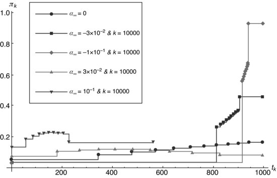
Table 8.1 The second column shows the cost of optimal trajectories for different values of the parameter ![]() . The third column is the cost calculated with a constant rate
. The third column is the cost calculated with a constant rate ![]() . Negative costs represent gains due to diminishing prices. Costs increase as
. Negative costs represent gains due to diminishing prices. Costs increase as ![]() increases
increases
| Cost – Optimal ($) | Cost at 10 % ($) | |
| 0 | −5953.5 | 6266.72 |
| −6082.71 | 721.25 | |
| −37608.9 | −12218. | |
| −8969.41 | 11812.2 | |
| 10−1 | 12982.5 | 24751.6 |
8.4.1.2 Very high urgency
Figure 8.2 The figure shows optimal execution trajectories for very rapid alpha decay: ![]() . The two trajectories
. The two trajectories ![]() and
and ![]() coincide on this graph: an aggressive trade start is only optimal when short-term alpha is large enough to outweigh the additional impact cost. The value
coincide on this graph: an aggressive trade start is only optimal when short-term alpha is large enough to outweigh the additional impact cost. The value ![]() is the critical point for the “phase change”, where the trajectory changes radically and stops behaving as
is the critical point for the “phase change”, where the trajectory changes radically and stops behaving as ![]() .
.
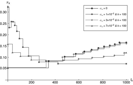
Table 8.2 The costs of the optimal schedule is shown in comparison to the 10 % strategy for different levels of short-term alpha in the case of very rapid alpha decay. Costs increase as ![]() increases; schedule optimization offers little room for profit in this case because alpha decays too rapidly in relation to the trade size: there is too little time to trade
increases; schedule optimization offers little room for profit in this case because alpha decays too rapidly in relation to the trade size: there is too little time to trade
| Cost – Optimal ($) | Cost at 10 % ($) | |
| 0 | 5953.5 | 6266.72 |
| 17945.1 | 18325.5 | |
| 9689.93 | 9884.37 | |
| 14686.5 | 14707.9 |
8.4.1.3 High urgency
Figure 8.3 This is a case ![]() . For
. For ![]() , trajectories are qualitatively very similar to the one for
, trajectories are qualitatively very similar to the one for ![]() . The case
. The case ![]() marks the transition from back-loaded schedules to front-loaded ones when short-term alpha is larger. In the extreme case where short-term alpha is 100 bps (
marks the transition from back-loaded schedules to front-loaded ones when short-term alpha is larger. In the extreme case where short-term alpha is 100 bps (![]() , the high expectation of increasing prices suggests a fast start and a short trading time (about 36 % of TM). Immediately, the optimization decreases the rate by 10 % to compensate for the impact costs. It follows a monotonous increase of more than 10 % in a lapse of
, the high expectation of increasing prices suggests a fast start and a short trading time (about 36 % of TM). Immediately, the optimization decreases the rate by 10 % to compensate for the impact costs. It follows a monotonous increase of more than 10 % in a lapse of ![]() of the total trading time. Finally, it reduces by 10 % to a constant rate during
of the total trading time. Finally, it reduces by 10 % to a constant rate during ![]() of the time, until the end. Those rises and falls in the participation rate are the efforts of the optimization to reach an equilibrium between impact and alpha term increments.
of the time, until the end. Those rises and falls in the participation rate are the efforts of the optimization to reach an equilibrium between impact and alpha term increments.
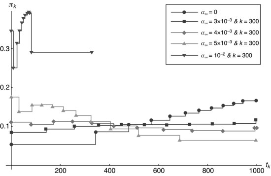
Table 8.3 Optimal costs are compared to the 10 % participation strategy for the case of moderately rapid alpha decay. The 10 % strategy is close to optimal for the most common alpha values, 30–50 bps. Back-loaded schedules are more economical when expectations are balanced; front-loading provides significant benefits for short-term alpha values in excess of 60 bps
| Cost – Optimal ($) | Cost at 10 % ($) | |
| 0 | 5953.5 | 6266.72 |
| 10−2 | 14912.4 | 16225.3 |
| 9248.68 | 9254.29 | |
| 10241.5 | 10250.2 | |
| 11175.6 | 11246 | |
| 12037.2 | 12241.9 |
8.4.1.4 Moderate urgency
Figure 8.4 This is the case ![]() . Even for the high
. Even for the high ![]() scenario,
scenario, ![]() , it is optimal to extend the execution over the entire window to minimize impact costs.
, it is optimal to extend the execution over the entire window to minimize impact costs.
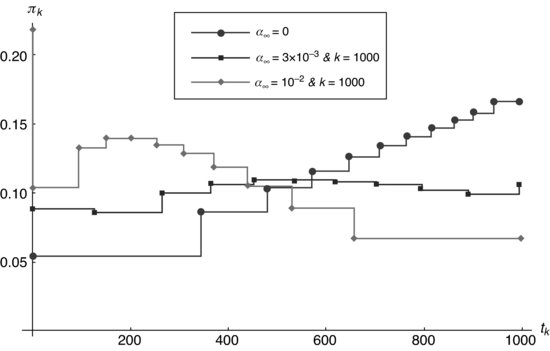
Table 8.4 The costs of optimal solutions are compared to the 10 % participation strategy for different short-term alpha expectations; the 10 % strategy is near optimal when the expected short-term alpha is 30 bps
| Cost – Optimal ($) | Cost at 10% ($) | |
| 0 | 5953.5 | 6266.72 |
| 7987.48 | 8003.97 | |
| 10−2 | 11348 | 12057.5 |
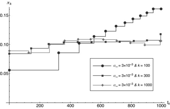
8.4.1.5 Graph comparison between different time decay constants
Figure 8.5 Very strong momentum.
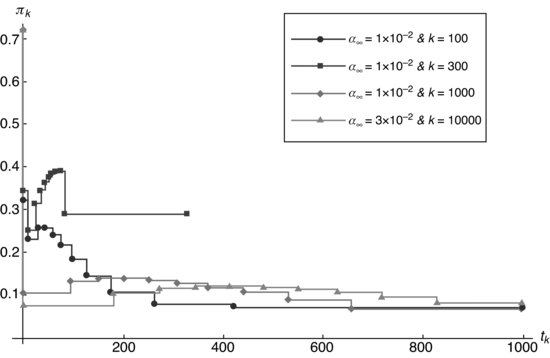
Figure 8.6 Moderate momentum.
8.4.2 Risk-adjusted optimization
Above, we finished the analysis of the hidden order arbitrage theory for variable speed of trading with zero risk aversion ![]() . In what follows, we will be concentrating on finding the optimal trading trajectories for a theory with varying participation rate, alpha term zero, and arbitrary risk aversion. This means minimizing the total risk-adjusted cost function (8.16), with the constraints (8.11) and (8.12).
. In what follows, we will be concentrating on finding the optimal trading trajectories for a theory with varying participation rate, alpha term zero, and arbitrary risk aversion. This means minimizing the total risk-adjusted cost function (8.16), with the constraints (8.11) and (8.12).
Figure 8.7 Critical momentum. It is optimal to front-load the execution schedule when the momentum is at least 60 bps or 70 bps, depending on the time decay parameter.
If we take an annual volatility of 30 %, ![]() . In our case, we work with transaction units as a measure of time and
. In our case, we work with transaction units as a measure of time and ![]() is the average number of a market transactions in each detectable interval. If one day consists of 6 hours and 30 minutes and each detectable interval last 15 minutes, then 1 day = 2600 market transactions. Therefore,
is the average number of a market transactions in each detectable interval. If one day consists of 6 hours and 30 minutes and each detectable interval last 15 minutes, then 1 day = 2600 market transactions. Therefore, ![]() .
.
The shortfall of risk-adjusted cost optimal solutions is listed in Table 8.5. For this example and different risk aversion parameters, ![]() is the corresponding dimensionless risk parameter.
is the corresponding dimensionless risk parameter.
Table 8.5 Shortfall of risk-adjusted cost optimal solutions. We consider a mid-cap trade of 25 000 shares, in an S0=$ 50 security, executed at an average participation rate of 10 % (![]() . If the security's trading volume is 400 transactions/h, a detectable interval will represent 15 minutes of trading. The impact for a 15-minute interval is estimated to be 10 bps for this security, i.e.
. If the security's trading volume is 400 transactions/h, a detectable interval will represent 15 minutes of trading. The impact for a 15-minute interval is estimated to be 10 bps for this security, i.e. ![]() . We take an annual volatility of 30 % or
. We take an annual volatility of 30 % or ![]() . One day consists of 6 hours and 30 minutes or 2600 market transactions. Results are for
. One day consists of 6 hours and 30 minutes or 2600 market transactions. Results are for ![]() , for the different values of the dimensionless risk constant
, for the different values of the dimensionless risk constant ![]() . The sixth column
. The sixth column ![]() is the total number of detectable intervals realized by the hidden order. The last column indicates that the number of market transactions reaches the maximum limit TM
is the total number of detectable intervals realized by the hidden order. The last column indicates that the number of market transactions reaches the maximum limit TM
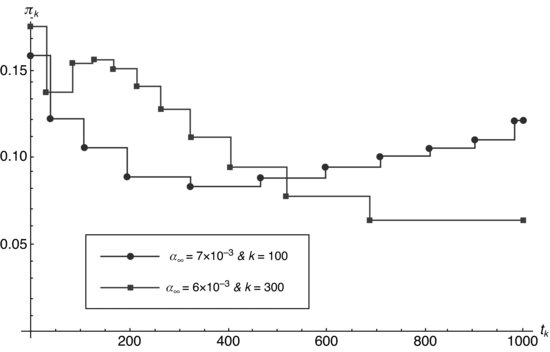
Figure 8.8 Optimal trajectories representing the participation rate in a function of the number of the detectable intervals for different values of the risk constant and ![]() .
.
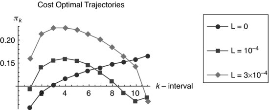
Figure 8.9 Participation rate in a function of the transactional time, ![]() , corresponding to each k interval, considering zero risk aversion and the alpha term.
, corresponding to each k interval, considering zero risk aversion and the alpha term.
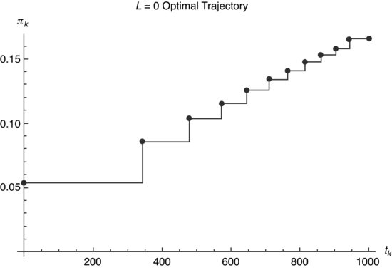
Figure 8.10 Participation rate in a function of the transactional time, ![]() , corresponding to each k interval, considering risk aversion
, corresponding to each k interval, considering risk aversion ![]() and
and ![]() .
.
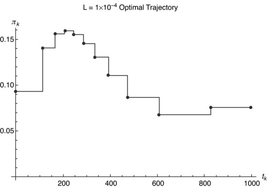
Figure 8.11 Participation rate in a function of the transactional time, ![]() , corresponding to each k interval, considering risk aversion
, corresponding to each k interval, considering risk aversion ![]() and
and ![]() .
.
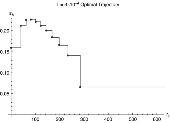
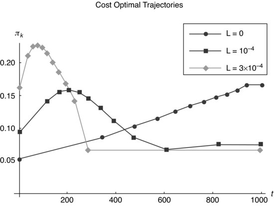
Figure 8.12 Comparative graph of optimal trajectories in a function of the transactional time for the different values of the risk aversion and ![]() in the quadratic approximation or continuum.
in the quadratic approximation or continuum.
In Figure 8.8 we graph the participation rate ![]() versus the detectable step k, in a continuum aproximation, for the different values of the risk constant
versus the detectable step k, in a continuum aproximation, for the different values of the risk constant ![]() and the nule alpha term.
and the nule alpha term.
Because in each step the participation rate must be constant, we present a detailed graph (see Figures 8.9, 8.10, and 8.11) of the participation rate versus the transactional time, ![]() , corresponding to each k interval, for each L. In Figure 8.12, we draw the comparative graph for the different values of the risk aversion in the quadratic approximation or continuum.
, corresponding to each k interval, for each L. In Figure 8.12, we draw the comparative graph for the different values of the risk aversion in the quadratic approximation or continuum.
8.5 CONCLUSIONS
Using hidden order arbitrage theory, we derived execution schedules that are optimal with respect to different optimization objectives: first, minimizing implementation shortfall with short-term alpha decay profiles typical of real-world trading situations and, second, minimizing the risk-adjusted shortfall to short-term alpha.
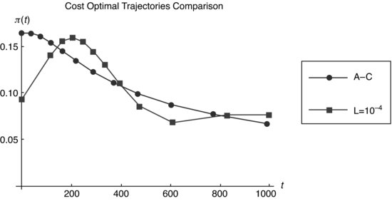
Figure 8.13 Comparative graph of the cost optimal trajectories in a function of the transactional time. The dot line is the solution predicted by the Almgren–Chriss formulation with linear impact and the risk-averse constant ![]() . The square line is the optimal trajectory for the nonlinear information arbitrage theory, as shown in Figure 8.10, for the risk-averse constant L=10−4 or
. The square line is the optimal trajectory for the nonlinear information arbitrage theory, as shown in Figure 8.10, for the risk-averse constant L=10−4 or ![]() .
.
8.5.1 Main results in the absence of short-term alpha
Shortfall minimization in the absence of alpha requires back-loading the execution schedule. This increases execution risk. Introducing risk aversion in the utility function, we found that optimal solutions for risk-averse traders move the schedule forward but avoid the aggressive trade start of the Almgren–Chriss (2000) solution. This suggests that hidden order arbitrage theory assigns a high cost to the signaling risk associated with an aggressive start of trading. In Figure 8.13 we graph the optimal risk averse trajectories for the information arbitrage theory with L=10−4 in comparison to Almgren and Chriss (2000). For a buy,
The shortfall calculated with the Almgren and Chriss (2000) trajectory for a risk-averse constant λ (Almgren–Chriss) = 10−5/$ is ![]() . This is 5.5 % costlier than the shortfall E(optimal)=$ 6520.5 for
. This is 5.5 % costlier than the shortfall E(optimal)=$ 6520.5 for ![]() , and 9.8 % costlier than a constant 10 % participation rate strategy.
, and 9.8 % costlier than a constant 10 % participation rate strategy.
8.5.2 Main results with short-term alpha
Short-term alpha is the expected impact-free return given the existence of a portfolio manager's order, i.e., the expected return if the institutional order is not executed. The existence of short-term alpha is an example of semi-strong market efficiency, because it is associated with the creation of an institutional order, which in itself constitutes private information. There are several reasons why this information should be associated with short-term alpha. First, portfolio managers may act coherently, either because they are following trading styles that are currently in fashion or because they are placing orders in response to shared signals such as analyst reports. In this case, the existence of one institutional order predicts an imbalance between institutional supply and demand associated with the possibility of other orders. Second, the market may price a security away from fair value because the liquidity demand from another portfolio manager creates a risk of liquidity exhaustion. This may happen in either direction; persistent selling creates a risk that market makers will withdraw their bids or a persistent buying pressure may force liquidity providers to cover short positions. In both cases, information about the creation of an institutional order on the contra side removes the liquidity exhaustion risk and causes price to revert to fair value. The third case where short-term alpha may occur is that of news-triggered trades, either in regard to intraday news or for orders placed before the open following overnight news.
The optimal execution schedule depends on how quickly alpha decays over time. In this chapter, we considered the optimal execution problem with exponential alpha decay profiles with low, moderate, or high urgency. High urgency represents alpha decay timescales of 10–30 % of the execution horizon, in moderate urgency the decay timescale is similar to the execution horizon, while in low urgency cases the alpha decay is quasi-linear during the execution horizon.
In the moderate urgency case, we found cost-optimal strategies that are front-loaded similarly to the optimal solution from hidden order arbitrage theory with risk aversion and no alpha. In the case of high urgency, for moderate short-term alpha values there is no benefit from front-loading because there is not enough time to complete a substantial part of the trade before alpha decays, and attempting to do so would increase impact costs for the remainder of the trade. It is only profitable to front-load the execution for the strongest short-term alpha profiles (>50 bps). In the case of negative alpha, typical of value managers, the optimal trading strategies begin slowly and increase participation near the end of the trading session.
8.5.3 Institutional trading practices
Comparing our results to the prevalent practices at institutional trading desks, we find two significant differences in the trading solutions:
Both deviations have the effect of reducing execution risk but increasing trading costs on average. We speculate that the preference of the industry for risk aversion is motivated, in part, by imperfect communication between the portfolio manager and the trading desk. In the absence of a precise understanding of what the trading desk is executing, portfolio managers naturally respond asymmetrically, making the desk responsible for large negative results and not offering a symmetric praise for large positive results. It is worth noting that a large positive result for the trading desk (buying far below the arrival price, for example) in general occurs when the portfolio manager's decision was mistimed in the short term (a buy order preceding a large drop in the price, or vice versa). Trading desks are not usually expected to question the wisdom of the portfolio manager's decision; the institutional trader's task is to execute the trade close to the arrival price. For that reason, the desk is unlikely to hear from the manager if it executed a poorly timed trade too fast, but far more likely to hear of a good trading decision that was executed too slowly. For the same reasons, a similar economic distortion exists for broker-dealers handling institutional orders. Another cause contributing to the problem is that the broker-dealer is compensated by commissions on executed shares; this creates an additional incentive to start executions quickly to lock in the commission before the order can be canceled.
Ultimately, it is the aggregate shortfall and not execution risk that impacts the fund performance. The additional cost from excessive front-loading can contribute significantly to fund rankings. For example, a 10 bps reduction in trading costs would translate to an improvement of 10 places in Bloomberg's ranking of US mutual funds in the “balanced” category. There are 1364 funds in that category for which a one-year rate of returns is reported.
The economic distortions that cause excessive risk aversion could be rectified if institutional desks were able to measure trading costs effectively and rate execution providers accurately. Unfortunately, post-trade data analysis is complicated by the difficulty of estimating opportunity costs. Limit prices clearly bias filled orders toward lower shortfalls, but occasionally lead to incomplete executions. The opportunity cost of the unfilled shares must be accounted for to evaluate the results. However, to measure opportunity costs accurately, one would need to know how the manager reallocated the funds that were not invested in the trade. For larger trades, it is common to execute over a period of weeks or even months. The trade size is likely to be adjusted multiple times and the adjustments themselves depend on the progress in executing the trade. Finally, selection bias plays a large role in that easier trades can be sent to lower quality algorithms where order flow is used as currency for paying brokers, while difficult trades are more likely to be sent to sophisticated execution systems. Trading desks are aware of these issues and mostly ignore post-trade TCA unless it is part of their compensation, relying instead on their experience to evaluate execution quality.
It is possible to account fairly for opportunity costs for the purpose of comparing the quality of execution from different algorithms. One need only compare the number of shares filled to the number that would have been filled had the algorithm performed at the intended speed. The difference can be priced at the estimated average price that would have been incurred had the trade been allowed to continue. This may not accurately measure opportunity cost from the perspective of the portfolio manager, who has other investment options, but it accounts fairly for the failure of an algorithm to perform. A framework to measure separately the effects of trading speed, algorithm performance, and limit prices was presented in Gomes and Waelbroeck (2010), for example. Unfortunately, the implementation of this type of framework in post-trade TCA is complicated by the fact that post-trade data rarely include the limit price, intended trading speed, or type of algorithm. However, these difficulties do not lessen the value of increased portfolio returns from optimal execution.
PROVISO
Aritas Group, Inc. and its subsidiary, Aritas Securities LLC, are members of FINRA/SIPC. This chapter was prepared for general circulation and without regard to the individual financial circumstances and objectives of persons who receive or obtain access to it. The analyses discussed herein are derived from Aritas and third party data and are not meant to guarantee future results.
REFERENCES
Almgren, R. (2003) Optimal Execution with Nonlinear Impact Functions and Trading-Enhanced Risk, Applied Mathematical Finance 10, 1–18.
Almgren, R. and N. Chriss (2000) Optimal Execution of Portfolio Transactions, Journal of Risk 3(2), 5–39.
Almgren, R., C. Thum, E. Hauptmann and H. Li (2005) Direct Estimation of Equity Market Impact, Risk 18, 57–62.
Bertismas, D. and A. Lo (1998) Optimal Control of Execution Costs, Journal of Financial Markets 1, 1–50.
Bouchaud, J.-P., J.D. Farmer and F. Lillo (2008) How Markets Slowly Digest Changes in Supply and Demand, in Handbook of Financial Markets: Dynamics and Evolution, T. Hens and K. Schenk-Hoppe (Eds), North-Holland, Elsevier, pp. 57–156.
Chan, L.K.C. and J. Lakonishok (1993) Institutional Trades and Intraday Stock Price Behavior, Journal of Financial Economics 33, 173–199.
Chan, L.K.C. and J. Lakonishok (1995) The Behavior of Stock Prices around Institutional Trades, Journal of Finance 50, 1147–1174.
Criscuolo, A.M. and H. Waelbroeck (2010) Optimal Execution in Presence of Hidden Order Arbitrage, Aritas Preprint PIPE-2011-01.
Farmer, J.D., A. Gerig, F. Lillo and H. Waelbroeck (2011) How Efficiency Shapes Market Impact, arXiv: 1102.5457v2[q-fin.TR].
Gabaix, X., P. Gopikrishnan, V. Plerou and H.E. Stanley (2006) Institutional Investors and Stock Market Volatility, Quarterly Journal of Economics 121, 461–504.
Gomes, C. and H. Waelbroeck (2008) Effect of Trading Velocity and Limit Prices on Implementation Shortfall, Aritas Group Preprint PIPE-2008-09-003.
Gomes, C. and H. Waelbroeck (2010) Transaction Cost Analysis to Optimize Trading Strategies, Journal of Trading, Fall 5(4).
Gopikrishnan, P., V. Plerou, X. Gabaix and H.E. Stanley (2000) Statistical Properties of Share Volume Traded in Financial Markets, Physical Review E 62(4), R4493–R4496.
Hora, M. (2006) The Practice of Optimal Execution. Algorithmic Trading 2, 52–60.
Lillo, F., J.D. Farmer and R.N. Mantegna (2003) Econophysics–Master Curve for Price-Impact Function, Nature 421(6919), 129.
Loeb, T.F. (1983) Trading Cost: The Critical Link between Investment Information and Results, Financial Analysts Journal 39(3), 39–44.
Moro, E., L.G. Moyano, J. Vicente, A. Gerig, J.D. Farmer, G. Vaglica, F. Lillo and R.N. Mantegna (2009) Market Impact and Trading Protocols of Hidden Orders in Stock Markets, Technical Report.
Obizhaeva, A. and J. Wang (2006) Optimal Trading Strategy and Supply/Demand Dynamics, Technical Report, AFA 2006 Boston Meetings Paper.
Torre, N. (1997) Market Impact Model Handbook, Barra Inc., Berkeley.
1 If order flow were a random walk with a bias π between buy and sell transactions, the imbalance would be detected with t-stat=1 after ![]() transactions.
transactions.