7

Collective Portfolio Optimization in Brokerage Data: The Role of Transaction Cost Structure

Damien Challet and David Morton de Lachapelle

7.1 INTRODUCTION

Regarding financial market behavior as a result of the interaction between many traders, i.e., as collective phenomena, opens the way to applying concepts and tools of statistical physics. In the last few decades, the latter has developed a powerful mathematical machinery that is able to solve the macroscopic dynamics resulting from the nonlinear microscopic interaction of fully heterogeneous adaptive complex agents, no less. One usually starts from known microscopic behavior and interaction and then study and possibly solve the resulting collective dynamics. In the case of financial markets, the lack of knowledge about the agents themselves hinders progress in this field. On the one hand, experimental psychology and behavioral finance put forward a picture of trader minds and actions that does not resemble many rational agents. On the other hand, the actual behavior of traders is seldom studied. Thus, one attempts to reverse engineer markets with agent-based models, trying painstakingly to guess what microscopic mechanism is necessary to reproduce a set of macroscopic stylized facts one observed in available data.

There has been some notable progress so far from statistical physicists. A quite important one is about volatility clustering. In game theory, giving the players the ability not to take part in a given game gives rise to much richer phenomenology (Szabó and Hauert, 2002). In the context of financial market models, letting the traders be active or inactive according to an indicator that fluctuates is enough to give rise to a long-term memory of the collective activity, and thus of volatility (Bouchaud et al., 2001). In other words, including this ingredient in an agent-based model guarantees the production of clustered volatility (see, for example, Johnson et al., 2000; Giardina and Bouchaud, 2003; Challet, 2007; Challet et al., 2005a). Another contribution is to relate the onset of large fluctuations to a phase transition between unpredictable and predictable price dynamics (Challet et al., 2005b).

The problem with this approach is that simple mechanisms may not be sufficient to understand and replicate the full complexity of financial markets, as some part of it may lie instead in the heterogeneity of the agents themselves. While the need for heterogeneous agents in this context is intuitive (see, for example, Arthur, 1994), there is no easily available data against which to test or to validate microscopically an agent-based model. Even if it is relatively easy to design agent-based models that reproduce some of the stylized facts of financial markets (see, for example, Challet et al., 2005b; Lux and Marchesi 1999; Caldarelli et al., 1997; Brock and Hommes, 1997; Alfarano and Lux, 2003), one never knows if this is achieved for good reasons. In addition, it is to be expected that real traders behave sometimes at odds with one's intuition.

Hence the need for data on trader behavior, which are usually hard to obtain; brokers of course have some data, but these are not easily accessible. Quite tellingly, this lack of data is not entirely to blame for the current ignorance of real-trader dynamics: researchers, even when given access to broker data, tend to focus on trading gains and behavioral biases (see, for example, Barber et al., 2004; Bauer et al., 2007; Dea et al., 2010).

The aim of this contribution is to show that a simple law of collective (read average) behavior of a population of traders, with large individual fluctuations, can be found when plotting the average transaction value against the average portfolio value of each agent, for the whole population of traders. The collective behavior we report here reflects to a large extent mean-variance portfolio optimization with transaction cost.

7.2 DESCRIPTION OF THE DATA

Our dataset is extracted from the database of the largest Swiss on-line broker, Swissquote Bank SA (further referred to as Swissquote). The sample contains comprehensive details about all 19 million electronic orders sent by 120 000 professional and nonprofessional on-line traders from January 2003 to March 2009. Of these orders, 65 % have been cancelled or have expired and 30 % have been filled; the remaining 5 % were still valid as of the 31 March 2009. Since this study focuses on the transaction value as a function of the account value, we chose to exclude orders for products that allow traders to leverage their investments, i.e., orders to margin-calls markets such as the foreign exchange market (FOREX) and the derivative exchange (EUREX). The resulting sample contains 540 % of orders for derivatives, 420 % for stocks, and 4 % for bonds and funds. Finally, 70 % of these orders were sent to the Swiss market, 20 % to the German market, and about 10 % to the US market.

Swissquote clients consist of three main groups: individuals (or retail clients), companies, and asset managers. Individual traders are mainly nonprofessional traders acting for their own account. The account of a company is usually managed by an individual trading on its behalf and, as we shall see, behaves very much like retail clients, albeit with a larger typical account value. Finally, asset managers manage accounts of individuals and/or companies, some of them dealing with more than a thousand clients.

7.3 RESULTS

For each trader i, we determine the days of trading activity tk, and define the average portfolio value on the days before the transactions took place, i.e., . The average transaction value, denoted by Ti, is defined as the price paid times the volume of the transaction and does not include transaction fees. We have excluded the traders who have leveraged positions on stocks, and hence .

We first produce a scatter plot of versus (Figure 7.1). In a log-log scale plot, it shows a cloud of points that is roughly increasing. A density plot is, however, clearer for retail clients as there are many more points (Figure 7.2).

Figure 7.1 Scatter plot of the average log T versus the average log Pv, robust nonparametric fit (solid line) and linear fits (dashed lines).

These plots make it clear that the average relationship between log T and log Pv is rather simple. A robust nonparametric regression method (Cleveland and Devlin, 1988) reveals a double linear relationship between and (see Figures 7.1 and 7.2) that can be formalized as

(7.1)

where x=1 when and x=2 when . Fitted values with confidence intervals are reported in Table 7.1.

Remarkably, the transition occurs at roughly the same values of for the three categories of traders; in addition, the slopes of these lines are very similar. This begs for a generic explanation, which, we argue below, is to be found in the collective tendency of Swissquote on-line traders to hold mean-variance portfolios that take into account the effective broker transaction fee structure of Swissquote, which has also two regions.

The relationships above only applies to local averages over all the agents. Regression residuals are for the most part (i.e. more than 95 %) normally distributed with constant standard deviations , without fat tails. This directly suggests the following simple relation for individual traders

(7.2)

Figure 7.2 Density plot of the average log T versus the average log Pv, robust nonparametric fit (solid line) and linear fits (dashed lines).

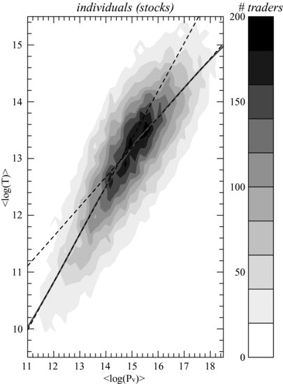
Table 7.1 Parameter values and 95 % confidence intervals for the double linear model (7.2). For each category of investors, the first and second rows correspond respectively to and . For confidentiality reasons, we have multiplied Pv and T by a random number. This only affects the true values of ax and Θ in the table

where Ti and Piv are respectively the turnover and portfolio value of investor i and are i.i.d. idiosyncratic variations independent from Pv that mirror the heterogeneity of the agents. As we shall see, portfolio optimization with heterogeneous parameters yields this precise relationship.

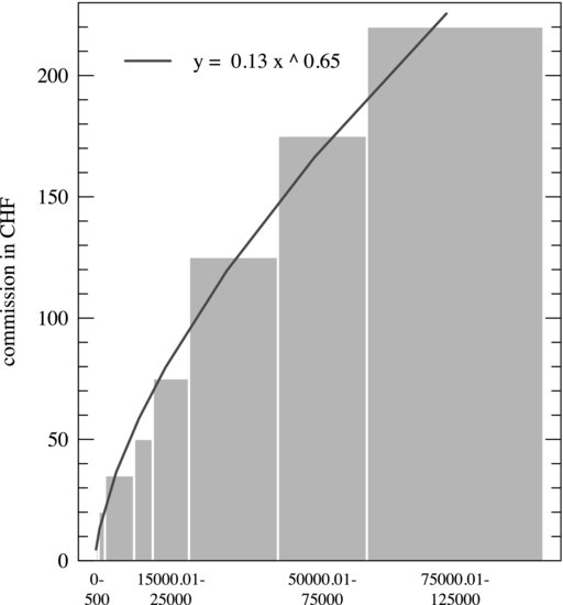
Figure 7.3 Swissquote fee curve for the Swiss stock market. Commissions based on a sliding scale of costs are common practice in the world of on-line finance. The solid line results from a nonlinear fit to Equation (7.4). Parameter values are and , where the 95 % confidence intervals are obtained from the BCa bootstrap method of Efron and Tibshirani (1993).

7.4 THE INFLUENCE OF TRANSACTION COSTS ON TRADING BEHAVIOR FROM OPTIMAL MEAN-VARIANCE PORTFOLIOS

As hinted above, we will argue that the origin lies in the Swissquote fee structure, which is shown in Figure 7.3; it is a piecewise constant, nonlinear looking function and flat for transactions larger than some given value. Fitting all increasing segments to Equation (7.4) gives .

In order to understand the influence of this peculiar transaction cost structure not accounted for in the literature, we need to derive simple portfolio optimization results. The simplest setting is found in Brennan (1975): it is a one-shot portfolio mean-variance optimization. The function to minimize is

(7.3)

where R is the stochastic return of the portfolio over the investment time horizon and λ is the relative importance of return with respect to risk. The return of the portfolio can be decomposed into contributions from risky assets, the interests of the amount kept in cash, and the total relative cost of broker commission, which we denote as R = Rrisky + Rcash − Rcost. More precisely.

• Rrisky = , where Ri is the return of stock i over this horizon, xi is the fraction of the total wealth invested in this stock, and N is the total number of investable assets; we shall denote the total fraction of wealth invested in risky assets by .
• Rcash = (1−x)r, where r is the interest rate.
• Rcost = , where F(x) is the amount charged by a broker to exchange an amount x of cash into shares or vice versa.

The fees structure of Swissquote is approximated by a power function law until up to F=Fmax and then a constant value. We hence choose

(7.4)

where δ interpolates between a flat-fee (), as in Brennan (1975), and a proportional scheme () via a power function law, and C is a constant. We assume that the return of asset i follows a one-factor model (Sharpe, 1964)

(7.5)

where is an uncorrelated white noise and the factor associated to asset i. This is a surprisingly good approximation to Swiss securities price dynamics.

Assuming an equally weighted portfolio, xi=x/N is constant for all i and we are left with only four parameters x, N, δ, and λ; since all the transactions have the same value, there is no risk to hit the two regions of Swissquote fee structure within a single portfolio, and hence δ is constant. We are mostly interested in N as a function of x. The technical details can be found in Morton de Lachapelle and Challet (2010). One finally finds that

(7.6)

where K is the ratio of residual risk to market risk, defined as

(7.7)

Given the desired level of investment x, (7.6) can be solved for N numerically in an actual portfolio optimization. Further insight is gained by considering the high diversification limit (or, equivalently, the high portfolio value limit), which yields in (7.6) and thus

(7.8)

where K is given by the right-hand side of (7.7). The latter equation generalizes (Brennan, 1975) to the case of a varying cost impact, represented here by the parameter δ (i.e. the result of Brennan, 1975, is recovered by setting and in (7.8)). These results can be to some extent generalized to nonequally weighted portfolios.

In essence, (7.8) says that the number of securities held in an equally weighted mean-variance portfolio with Sharpe-like returns is related to the amount invested as

(7.9)

in the high diversification limit, where κ is the pre-factor of in (7.8). The last equation gives N as a function of Pv for a pre-defined x in the optimal portfolio. The heterogeneity of the traders, beyond their account value, is not apparent yet, but may occur both in x and κ: first each trader may have his own preference regarding the fraction of this account to invest in risky assets, x; therefore one should replace x by xi; next, κ includes both a term related to transaction costs, which does vary from trader to trader, and some measures and expectation of market returns and variance; each trader may have his own perception or way of measuring them, and hence κ should also be replaced by . Finally, both terms can be merged in the same constant term . This explains how the heterogeneity of the traders is a cause of fluctuations in the kind of relationships we are interested in.

The result above only links the number of securities in a portfolio N with its value Pv, but one of course wishes to obtain relationships that involve the turnover per transaction, T, in order to compare Equation (7.9) with the empirical results of Section 7.3. One problem we face is that the portfolio optimization setup rests on the assumption that the agents build their portfolio by selecting a group of assets and stick to them over a period of time. This, obviously, does not include the possibility of speculating by a series of buy and sell trades on even a single asset, nor portfolio re-balancing, which consists in adjusting the relative proportions of some assets, all of which are in the data we have used in Section 7.3.

We have found a simple and effective method to select portfolio-building transactions: it consists in assuming that the latter include only the very first transaction of assets not traded previously; sell orders are ignored as Swissquote clients cannot short sell easily. In other words, if trader i owns some shares of assets A, B, and C and then buys some shares of asset D, this last transaction is deemed to contribute to his portfolio building process; the set of such transactions is denoted by , while the full set of transactions is denoted by . Subsequent transactions of shares of assets A, B, C, or D do not belong to . The number of different assets that trader i owns is supposed to be , where |X| is the cardinal of set X; this approach assumes that a trader always owns shares in all the assets ever traded; surprisingly, this is the most common case.

Let us drop the index i and now focus on , the total transaction value that helped build his portfolio. We should first check how it is related to the total portfolio value Pv. Let us define , the account value of this trader averaged at the times at which he trades a new asset. Plotting against gives a cloudy relationship, as usual, but fitting it with gives for individuals, for asset managers, and for companies with an adjusted R2=0.99 in all cases. This relationship trivially holds with for the traders who buy all their assets at once, as assumed in the portfolio model. The traders who do not lie on this line either hold positions in cash (this line is then a lower bound) or do not build their portfolio in a single day: they pile up positions in derivative products or stocks whose price fluctuations are one cause of the deviations from the line. However, the fact that the slope is close to 1 means that the average fluctuation is zero and hence that on average traders do not make money from the positions taken on new stocks. The consequence of this is that log Pv can be safely replaced by in (7.9); thus, setting x=1,

(7.10)

The x=1 assumption is in fact quite reasonable. Most Swissquote traders do not use their trading account as savings accounts and are fully invested; we do not know what amount they keep on their other bank accounts.

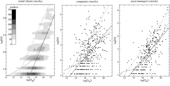
A robust nonparametric fit does reveal a linear relationship between log N and in a given region (Figure 7.4 overleaf). In this region, we have

Figure 7.4 Turnover of transactions contributing to the building of a portfolio versus the number N of assets held by a given trader at the time of the transaction. Light grey lines: nonparametric fit; dark grey lines: fits of the linear part of the nonparametric fit. From left to right: companies, asset managers, and individuals.

(7.11)

which gives

(7.12)

The fitted values are reported in Table 7.2. We still need to link and . While Section 7.3 showed that the unconditional averages lead to , one still finds that . Therefore, one can write

(7.13)

Table 7.3 contains the fitted parameters. Thus, one is finally rewarded with the needed link

(7.14)

which directly involves the transaction cost structure in the relationship between turnover and portfolio value, as argued in Section 7.3.1 This relationship allows us to close the loop as we are now able to relate directly the exponents linking T, N, and Pv. Going back to Section 7.3, this justifies the claim that the bilinear relationship between log turnover per transaction and log account value is linked to two values of δ.

Table 7.2 Slope α linking and log N for the three trader categories

Table 7.3 Results of the double linear regression of versus . For each category of investors, the first and second row correspond respectively to and , where have been determined graphically using the nonparametric method of Cleveland and Devlin (1988), as in Section 7.3. Parameters are as in the double linear model (7.2). For confidentiality reasons, we have multiplied Pv and T by a random number, which only affects the true values of and of the ordinate ax

The surprise comes from the precise value at which the transition occurs. Let us recall that the transitions between the standard Swissquote and an effective flat-fee structure occur at the same average value of T for the three categories of traders (idem for ). However, the real transition value of T is lower than 125 000 CHF (we cannot be more precise for confidentiality reasons). We propose two main reasons for this: first traders with a large account value negotiate a flat fee for all their transactions, leading to a simple and plausible explanation: most of the traders of the three categories who have a portfolio value larger than the transition value do have effectively a flat fee agreement. The other possibility is that the traders tend to either neglect, or regard as constant, transaction fees whose relative value is smaller than some threshold when they build their portfolio.

Let us finally discuss the empirical values of α, β, and δ against their theoretical counterparts, which are summarized in Table 7.4.

Table 7.4 Table summarizing the empirical and theoretical relationships between α, β, and δ

i. Small values of . It was impossible to measure α in that case since the nonparametric fit shows a nonlinear relationship in the log-log plot for retail clients, which we trust more since they have many more points than the graphs for the two other categories of clients. However, it may not make sense to expect a linear relationship since such a relationship is only expected for N large enough ( in practice) and a small is related to a small N. Hence we can only test . The reported value of β is consistent for all the clients. Retail clients have a larger δeff = than the estimated . Since the shape of the fee structure is not continuous, the values of these exponents can hardly be expected to match. However, fitting the whole curve structure may be problematic in this context: indeed, the traders with a typical small value of see a more linear relationship in the region of a small transaction value, which, when considering the whole curve – for instance, removing the two largest segments from the fee structure – yields , which is not far from δeff.

ii. Large values of . The relationships between all the exponents are verified for the three categories of clients. While uncertainties make the match not very impressive for companies and asset managers, this result is much stronger in the case of retail clients as relative uncertainties are small (1–2 %). The value of βretail is of particular interest as it corresponds to δeff = 0 or, equivalently, to a flat fee structure. Going back to the fees structure of Swissquote, one finds that the transition happens when the relative transaction cost falls below some threshold (we cannot give its precise value for confidentiality reasons; it is smaller than 1 %). A possible explanation is that either some traders with a high enough average turnover have a flat-fee agreement with Swissquote or that the rest of them simply act as if they were not able to take correctly into account transaction costs. Since not all traders have a flat-fee agreement, one must conclude that some traders disregard small relative fees. The reported value of β for companies and asset managers is larger that βretail, but it is more likely than not that the small sample size is responsible for this discrepancy, since these two categories of clients have a greater propensity to negotiate a flat-fee structure.

7.5 DISCUSSION AND OUTLOOK

We have been able to determine empirically a bilinear relationship between the average log-turnover per transaction and the average log-account value and have related it to the transaction fee structure of the broker and its perception by the agents. A theoretical derivation of optimal simple one-shot mean-variance portfolios with nonlinear transaction costs predicted relationships between turnover, number of different assets in the portfolio, and log-account values that could be verified empirically. This means that the populations of traders do take correctly on average, i.e., collectively, the transaction costs into account and act collectively as mean-variance equally weighted portfolio optimizers. This is not to say that each trader is a mean-variance optimizer, but that the population taken as a whole behaves as such – with differences across populations, as discussed in the previous section. This can be related to findings of Kirman's famous work on demand and offer average curves in Marseille's fish market (Härdle and Kirman, 1995) and more generally as what has become known as the wisdom of the crowds (see Surowiecki, 2005, for an easy-to-read account).

The fact that the turnover depends in a nonlinear way on the account value has important implications for agent-based models, which from now on must take into account the fact that the real traders do invest in a number of assets that depend nonlinearly on their wealth.

Future research will address the relationship between account value and trading frequency, which is of the utmost importance to understand if the many small trades of small investors have a comparable influence on the financial market than those of institutional investors. This will give an understanding of whom provides liquidity and what all the nonlinear relationships found above mean in this respect. This is also crucial in agent-based models, in which one often imposes such a relationship by hand, arbitrarily; conversely, one will be able to validate evolutionary mechanisms of an agent-based model according to the relationship between trading frequency, turnover, number of assets, and account value they achieve in their steady state.

ACKNOWLEDGMENTS

The authors thank the organizers of this stimulating conference. Swissquote Bank SA provided us with data and financial support to DMdL.

REFERENCES

Alfarano, S. and T. Lux (2003) A Minimal Noise Traders Model with Realistic Time Series Properties, in Long Memory in Economics, G. Teyssière and A.P. Kirman (Eds), Springer, Berlin.

Arthur, B.W. (1994) Inductive Reasoning and Bounded Rationality: The El Farol Problem, American Economic Review 84, 406–411.

Barber, B.M., Y.T. Lee, Y.J. Liu and T. Odean (2009) Just how much do individual investors lose by trading? Review of Financial Studies 22, 609.

Bauer, R., M. Cosemans and P. Eichholtz (2007) The Performance and Persistence of Individual Investors: Rational Agents or Tulip Maniacs?, http://papers.ssrn.com/sol3/papers.cfm?abstract_id=965810.

Bouchaud, J.-P., I. Giardina and M. Mézard (2001) On a universal mechanism for long ranged volatility correlations. Quantitative Finance 1, 212, cond-mat/0012156.

Brennan, M.J. (1975) The Optimal Number of Securities in a Risky Asset Portfolio When There are Fixed Costs of Transacting: Theory and Some Empirical Results, Journal of Financial and Quantitative Analysis 10(3), 483–496.

Brock, W.A. and C.H. Hommes (1997) A Rational Route to Randomness, Econometrica 65, 1059–1095.

Caldarelli, G., M. Marsili and Y.-C. Zhang (1997) A Prototype Model of Stock Exchange, Europhysics Letters 50, 479–484.

Challet, D. (2007) Inter-pattern Speculation: Beyond Minority, Majority and $-Games, Journal of Economics, Dynamics and Control (32), physics/0502140.

Challet, D., A. De Martino, M. Marsili and I.P. Castillo (2005a) Minority games with finite score memory, Journal of Experiment and Theory, P03004, cond-mat/0407595.

Challet, D., M. Marsili and Y.-C. Zhang (2005b) Minority Games, Oxford University Press, Oxford.

Cleveland, W.S. and S.J. Devlin (1988) Locally Weighted Regression: An Approach to Regression Analysis by Local Fitting, Journal of the American Statistical Association 83(403), 596–610.

Dea, S., N.R. Gondhib, V. Manglac and B. Pochirajud (2010) Success/Failure of Past Trades and Trading Behavior of Investors.

Efron, B. and R.-J. Tibshirani (1993) An Introduction to the Bootstrap, Chapman & Hall, New York.

Giardina, I. and J.-Ph. Bouchaud (2003) Crashes and Intermittency in Agent Based Market Models, European Physics Journal Series B, 31, 421–437.

Härdle, W. and A. Kirman (1995) Nonclassical Demand: A Model-Free Examination of Price-Quantity Relations in the Marseille Fish Market, Journal of Econometrics 67(1), 227–257.

Johnson, N.F., M. Hart, P.M. Hui and D. Zheng (2000) Trader Dynamics in a Model Market, ITJFA 3, cond-mat/9910072.

Lux, T. and M. Marchesi (1999) Scaling and Criticality in a Stochastic Multi-Agent Model of a Financial Market, Nature 397, 498–500.

Morton de Lachapelle, D. and D. Challet (2010) Turnover, Account Value and Diversification of Real Traders: Evidence of Collective Portfolio Optimizing Behavior, New Journal of Physics 12, 075039.

Sharpe, W.F. (1964) Capital Asset Prices: A Theory of Market Equilibrium Under Conditions of Risk, Journal of Finance 19(3), 425–442.

Surowiecki, J. (2005) The Wisdom of Crowds, Anchor Books, New York.

Szabó, G. and C. Hauert (2002) Phase Transitions and Volunteering in Spatial Public Goods Games, Physical Review Letters 89(11), 118101, August.

1 Note that this relationship can be obtained directly by assuming that all the transactions happen at the same time, and hence that T=(xPv)/N, which leads straightforwardly to (7.14).