
CHAPTER 3: Recursion
© Ake13bk/Shutterstock
This chapter introduces the topic of recursion—a distinct algorithmic problem-solving approach supported by many computer languages (Java included). What is recursion? Let us look first at a visual analogy.
You may have seen a set of brightly painted Russian dolls that fit inside one another. Inside the first doll is a smaller doll, inside of which is an even smaller doll, inside of which is yet a smaller doll, and so on. Solving a problem recursively is like taking apart such a set of Russian dolls. You first create smaller and smaller versions of the same problem until a version is reached that can no longer be subdivided (and that is easily solved)—that is, until the smallest doll is reached. Determining the overall solution often requires combining the smaller solutions, analogous to putting the dolls back together again.

Recursion, when applied properly, is an extremely powerful and useful problem solving tool. And it is fun! We will use it many times in upcoming chapters to support our work.
3.1 Recursive Definitions, Algorithms, and Programs
Recursive Definitions
You are already familiar with recursive definitions. Consider the following definition of the folder (or catalog, or directory) you use to organize files on a computer: A folder is an entity in a file system that contains a group of files and other folders. This definition is recursive because it expresses folder in terms of itself. A recursive definition is a definition in which something is defined in terms of smaller versions of itself.
Mathematicians regularly define concepts in terms of themselves. For instance, n! (read “n factorial”) is used to calculate the number of permutations of n elements. A nonrecursive definition of n! is

Consider the case of 4!. Because n > 0, we use the second part of the definition:
4! = 4 × 3 × 2 × 1 = 24
This definition of n! is not mathematically rigorous. It uses the three dots, rather informally, to stand for intermediate factors. For example, the definition of 8! is 8 × 7 × 6 × . . . × 1, with the . . . in this case standing for 5 × 4 × 3 × 2.
We can express n! more elegantly, without using the three dots, by using recursion:

This is a recursive definition because it expresses the factorial function in terms of itself. The definition of 8! is now 8 × 7!.
Recursive Algorithms
Let us walk through the calculation of 4! using our recursive definition. We use a set of index cards to help track our work—not only does this demonstrate how to use a recursive definition, but it also models the actions of a computer system executing a recursive program.
We take out an index card and write on it:

Looking at our recursive definition we determine that 4 is greater than 0, so we use the second part of the definition and continue writing:

Of course, we cannot complete the third line because we do not know the value of 3!. Before continuing with our original problem (calculating 4!), we have to solve this new problem (calculating 3!). So we take out another index card, stack it on top of our original card, and write down our new problem:

Again we look at our recursive definition. We determine that 3 is greater than 0, so we use the second part of the definition and continue writing:

As before, we cannot complete the third line because we do not know the value of 2!. We take out another index card and write down our new problem. Continuing in this way we eventually have five cards stacked on our desk:

At this point, when we turn to our recursive definition to calculate 0! we find that we can use the first part of the definition: 0! equals 1. We can complete the top card as shown here:

That finishes the problem at the top of our stack of cards. Its result is 1. Remembering that result, we throw away the top card, write the “1” into the empty slot on the card that is now on top (the Calculate 1! card), and continue working on that problem. Because we know how to calculate 1 × 1, we can quickly finish that problem and enter its result.

As before, we remember this result, discard the top card, enter the result onto the next card (the Calculate 2! card), and continue. In quick succession we determine that

ending with the solution to our original problem:

Note that we stopped creating new problem cards when we reached a case for which we know the answer without resorting to the recursive part of the definition. In this example, that point occurred when we reached Calculate 0!. We know that value is 1 directly from the definition without having to resort to recursion.
When the answer for a case is directly known, without requiring further recursion, it is called a base case. A recursive definition may have more than one base case. The case for which the solution is expressed in terms of a smaller version (or versions) of itself is called the recursive or general case. A recursive definition may also have more than one recursive case. A recursive algorithm is an algorithm that expresses a solution in terms of smaller versions of itself. A recursive algorithm must terminate; that is, it must have a base case, and the recursive cases must eventually lead to a base case.
Here is our recursive algorithm for calculating n! based directly on the recursive definition. It assumes that n is a nonnegative integer.
Recursive Programs
In Java, a method can invoke other methods. A method can even invoke itself. When a method invokes itself, it is making a recursive call. It is only natural to use recursive method calls to implement recursive-problem solutions.
Here is a Java method that corresponds to our recursive factorial algorithm. It uses a recursive call (emphasized) to calculate the factorial of its integer argument.
public static int factorial(int n)
// Precondition: n is nonnegative
//
// Returns the value of "n!"
{
     if (n == 0)
         return 1;       // Base case
     else
         return (n * factorial(n - 1));       // General case
}
The argument in the recursive call, n - 1, is different from the argument in the original call, n. This is an important and necessary condition; otherwise, the method would continue calling itself indefinitely.
Suppose, for example, an application with access to the above method invokes the following statement:
System.out.println(factorial(4));
Much the same as with our index card example above, when the system is executing factorial(4) it invokes factorial(3), that in turn invokes factorial(2), that in turn invokes factorial(1), that in turn invokes factorial(0) the base case. As you can see, the recursive calls lead to the base case where the chain of calls ends; otherwise it would recurse forever. At this point the chain of return statements begins, with factorial(0) returning 1, factorial(1) returning 1, factorial(2) returning 2, factorial(3) returning 6, and factorial(4) returning 24 which the application prints.
The factorial method is an example of direct recursion. Direct recursion is recursion in which a method directly calls itself. All of the examples in this chapter involve direct recursion. Indirect recursion is recursion in which a chain of two or more methods calls return to the method that originated the chain. For example, method A calls method B, and method B calls method A; the chain of method calls could be even longer, but if it eventually leads back to method A, then it is indirect recursion.
Iterative Solution for Factorial
Recursion is a powerful programming technique, but we must be careful when using it. Recursive solutions can be less efficient than iterative solutions to the same problem. In fact, some of the examples presented in this chapter, including factorial, are better suited to iterative approaches. This topic is discussed in depth in Section 3.8, “When to Use a Recursive Solution.”
We used the factorial algorithm to demonstrate recursion because it is familiar and easy to visualize. In practice, we would never want to solve this problem using recursion, as a straightforward, more efficient iterative solution exists. Here we look at the iterative solution to the problem:
public static int factorial2(int n)
// Precondition: n is nonnegative
//
// Returns the value of retValue: n!
{
      int retValue = 1;
      while (n != 0)
      {
         retValue = retValue * n;
         n = n - 1;
      }
      return(retValue);
}
Iterative solutions tend to employ loops, whereas recursive solutions tend to have selection statements—either an if or a switch statement. A branching structure is usually the main control structure in a recursive method. A looping structure is the corresponding control structure in an iterative method. The iterative version of factorial has two local variables (retValue and n), whereas the recursive version has none. There are usually fewer local variables in a recursive method than in an iterative method. The iterative solution is more efficient because starting a new iteration of a loop is a faster operation than calling a method. Both the iterative and the recursive factorial methods are included within the TestFactorial application in the ch03.apps package.
3.2 The Three Questions
This section presents three questions to ask about any recursive algorithm or program. Using these questions helps us verify, design, and debug recursive solutions to problems.
Verifying Recursive Algorithms
The kind of walk-through presented in Section 3.1, “Recursive Definitions, Algorithms, and Programs” (using index cards), is useful for understanding the recursive process, but it is not sufficient for validating the correctness of a recursive algorithm. After all, simulating the execution of factorial(4) tells us the method works when the argument equals 4, but it does not tell us whether the method is valid for other arguments.
We use the Three-Question Approach for verifying recursive algorithms. To verify that a recursive solution works, we must be able to answer yes to all three of these questions:
The Base-Case Question Is there a nonrecursive way out of the algorithm, and does the algorithm work correctly for this base case?
The Smaller-Caller Question Does each recursive call to the algorithm involve a smaller case of the original problem, leading inescapably to the base case?
The General-Case Question Assuming the recursive call(s) to the smaller case(s) works correctly, does the algorithm work correctly for the general case?
Let us apply these three questions to the factorial algorithm:
The Base-Case Question The base case occurs when n is 0. The
Factorialalgorithm then returns the value of 1, which is the correct value of 0! by definition. The answer is yes.The Smaller-Caller Question The parameter is n and the recursive call passes the argument n - 1. Therefore each subsequent recursive call sends a smaller value, until the value sent is finally 0, which is the base case. The answer is yes.
The General-Case Question Assuming that the recursive call
Factorial(n - 1)gives us the correct value of (n - 1)!, the return statement computes n * (n - 1)!. This is the definition of a factorial, so we know that the algorithm works in the general case—assuming it works in the smaller case. The answer is yes.
Because the answers to all three questions are yes, we can conclude that the algorithm works. If you are familiar with inductive proofs, you should recognize what we have done. Having made the assumption that the algorithm works for the smaller case, we have shown that the algorithm works for the general case. Because we have also shown that the algorithm works for the base case of 0, we have inductively shown that it works for any integer argument greater than or equal to 0.
Determining Input Constraints
For the factorial problem we assumed the original value for n is greater than or equal to 0. Note that without this assumption we cannot answer the smaller-caller question affirmatively. For example, starting with n = -5, the recursive call would pass an argument of -6, which is farther from the base case, not closer, as required.
These kinds of constraints often exist on the input arguments for a recursive algorithm. We can typically use our three-question analysis to determine these constraints. Simply check whether there are any starting argument values for which the smaller call does not produce a new argument that is closer to the base case. Such starting values are invalid. Constrain your legal input arguments so that these values are not permitted.
Writing Recursive Methods
The questions used for verifying recursive algorithms can also be used as a guide for writing recursive methods. Here is a good approach to designing a recursive method:
Get an exact definition of the problem to be solved.
Determine the size of the problem to be solved. On the initial call to the method, the size of the whole problem is expressed in the value(s) of the argument(s).
Identify and solve the base case(s) in which the problem can be expressed nonrecursively. This ensures a yes answer to the base-case question.
Identify and solve the general case(s) correctly in terms of a smaller case of the same problem—a recursive call. This ensures yes answers to the smaller-caller and general-case questions.
In the case of the factorial problem, the definition of the problem is summarized in the definition of the factorial function. The size of the problem is the number of values to be multiplied: n. The base case occurs when n is 0, in which case we take the nonrecursive path. The general case occurs when n > 0, resulting in a recursive call to factorial for a smaller case: factorial(n - 1). Summarizing this information in table form:
Debugging Recursive Methods
Because of their nested calls to themselves, recursive methods can be confusing to debug. The most serious problem is the possibility that the method recurses forever. A typical symptom of this problem is an error message telling us that the system has run out of space in the run-time stack, due to the level of recursive calls. (Section 3.7, “Removing Recursion,” looks at how recursion uses the run-time stack.) Using the Three-Question Approach to verify recursive methods and determine argument constraints should help us avoid this problem.
Success with the three questions does not guarantee, however, that the program will not fail due to lack of space. Section 3.8, “When to Use a Recursive Solution,” discusses the amount of space overhead required to support recursive method calls. Because a call to a recursive method may generate many levels of method calls to itself, the space consumed might be more than the system can handle.
One error that programmers often make when they first start writing recursive methods is to use a looping structure instead of a branching one. Because they tend to think of the problem in terms of a repetitive action, they inadvertently use a while statement rather than an if statement. The body of a recursive method should always break down into base and recursive cases. Hence, we use a branching statement. It is a good idea to double-check our recursive methods to make sure that we used an if or switch statement to select the recursive or base case.
3.3 Recursive Processing of Arrays
Many problems related to arrays lend themselves to a recursive solution. After all, a subsection of an array (a “subarray”) can also be viewed as an array. If we can solve an array-related problem by combining solutions to a related problem on subarrays, we may be able to use a recursive approach.
Binary Search
The general problem addressed in this section is finding a target element in a sorted array. Our approach is to examine the midpoint of the array and compare the element found there to our target element—if we are lucky they are “equal,” but even if not lucky we are able to eliminate half the array from further consideration depending on whether our target element is greater than or less than the examined element. We repeatedly examine the middle element in the remaining part of the array, eliminating half the remaining elements until we either find our target or determine that it is not in the array.
This approach is an example of the “decrease and conquer” algorithm design technique—we conquer the problem by decreasing the size of the array subsection to search at each stage of the solution process. The specific decrease and conquer algorithm used here is called the Binary Search algorithm.
Binary Search is a good fit for a recursive implementation. At the end of any stage in which the target is not located we continue by searching a portion of the original array— and we can use Binary Search to search that subarray.
Assume we have a sorted array of int named values that is accessible from within the recursive method binarySearch. Our specific problem is to determine if a given int named target is in the array. We pass our recursive method the target element and both the starting and ending indices of the portion of the array we are still searching. The signature for the method therefore is
boolean binarySearch(int target, int first, int last)
Here we use a specific example to help us add detail to our algorithm and create our code. Let us search for the value 20 in an array containing 4, 6, 7, 15, 20, 22, 25, and 27. At the beginning of our search first is 0 and last is 7; therefore we invoke binarySearch(20, 0, 7) resulting in

The midpoint is the average of first and last
midpoint = (first + last) / 2;
giving us the following:

If values[midpoint] (which is 15) equals target (which is 20) then we are finished and can return true. Unfortunately it does not. However, since values[midpoint] is less than target we know we can eliminate the lower half of the array from consideration. We set first to midpoint + 1 and recursively call binarySearch(20, 4, 7). A new midpoint is calculated resulting in

This time values[midpoint] is greater than target so we can eliminate the upper half of the remaining portion of the array from consideration. We set last to midpoint - 1 and recursively call binarySearch(20, 4, 4), again calculating a new midpoint, resulting in

Finally, values[midpoint]equals target so we are finished and can return true.
Through this example we have identified how to handle the cases where the element at array location midpoint is less than, greater than, and equal to target. But we still need to determine how to terminate the algorithm if the targeted element is not in the array.
Consider the above example again, but this time with 18 replacing 20 as the fifth element of values. The same sequence of steps would occur until at the very last step we have the following:

Continuing from this point we see that values[midpoint] is less than target so we set first to midpoint + 1 and recursively call binarySearch(20, 5, 4):

Note that we have eliminated the entire array from consideration and are invoking binarySearch with a first argument that is larger than the last argument. This is obviously a degenerate situation—attempting to search a space in the array that does not exist. It is in this situation where the method returns false, indicating that target is not in the array.
Here is a summary table for the algorithm:
Let us verify Binary Search using the Three-Question approach:
The Base-Case Question There are two base cases.
If
first > lastthe algorithm returnsfalse. This is correct because in this case there are no array elements to search.If
values[midpoint] == targetthe algorithm returnstrue. This is correct becausetargethas been found.
The answer is yes.
The Smaller-Caller Question In the general case
binarySearchis called with parametersfirstandlastindicating the start and end of a subarray to search, withfirst <= last. Because themidpointis calculated as(first + last)/2it must be>= firstand<= last. Therefore, the size of the ranges(midpoint+1, last)and(first, midpoint-1)must be less than the range(first, last). The answer is yes.The General-Case Question Assuming that the recursive calls
binarySearch(target, midpoint+1, last)andbinarySearch(target, first, midpoint-1)give the correct result, then thereturnstatement gives the correct result because it has already been determined thattargetcould not be in the other part of the array—whether or not it is in the array completely depends on whether or not it is in the indicated subarray. The answer is yes.
Because the answers to all three questions are yes, we can conclude that the algorithm works. Here is the code:
boolean binarySearch(int target, int first, int last)
// Precondition: first and last are legal indices of values
//
// If target is contained in values[first,last] return true
// otherwise return false.
{
   int midpoint = (first + last) / 2;
   if (first > last)
      return false;
   else
      if (target == values[midpoint])
         return true;
      else
      if (target > values[midpoint])  // target too high
         return binarySearch(target, midpoint + 1, last);
      else                           // target too low
         return binarySearch(target, first, midpoint - 1);
}
This code can be found in a file BinarySearch.java in the package ch03.apps. The code also includes an iterative version of the algorithm that is not much different than the recursive version. Note that this algorithm has already been analyzed for efficiency. It is O(log2N)—see the latter part of Section 1.6, “Comparing Algorithms: Order of Growth Analysis.”
3.4 Recursive Processing of Linked Lists
Arrays and linked lists (references) are our two basic building blocks for creating data structures. The previous section discussed some examples of recursive processing with arrays. This section does the same for linked lists. To simplify our linked list figures in this section, we sometimes use a capital letter to stand for a node’s information, an arrow to represent the link to the next node (as always), and a slash to represent the null reference.

Recursive Nature of Linked Lists
Recursive approaches often work well for processing linked lists. This is because a linked list is itself a recursive structure, even more so than the array. Section 2.7, “Introduction to Linked Lists” introduced the LLNode class, our building block for linked lists. It noted that LLNode is a self-referential class, indicating that an LLNode object contains a reference to an LLNode object as emphasized in the following code segment:
public class LLNode<T>
{
     protected T info;             // information stored in list
     protected LLNode<T> link;     // reference to a node
. . .
Self-referential classes are closely related to recursion. In a certain sense, they are recursive.
A linked list is either empty or consists of a node containing two parts: information and a linked list. For example, list1 is empty whereas list2 (the list containing A, B, and C) contains a reference to an LLNode object that contains information (A) and a linked list (the list containing B and C):

Note that the link value in the “last” node on the list is always null. When we process linked lists recursively, processing this null value is typically a base case.
Traversing a Linked List
Traversing a linked list in order to visit each element and perform some type of processing is a common operation. Suppose we wish to print the contents of the list. The recursive algorithm is straightforward—if the list is empty do nothing; otherwise, print the information in the current node, followed by printing the information in the remainder of the list (see Figure 3.1).

Figure 3.1 Printing a list recursively
Transforming this algorithm into code is also straightforward:
void recPrintList(LLNode<String> listRef)
// Prints the contents of the listRef linked list to standard output
{
   if (listRef != null)
   {
      System.out.println(listRef.getInfo());
      recPrintList(listRef.getLink());
   }
}
Within the if statement the content of the first node on the list pointed to by listRef is printed, followed by the recursive call to recPrintList that prints the remainder of the list. Our base case occurs when we reach the end of the list and listRef is null, in which case the if statement is skipped and processing stops. Here we verify recPrintList using the Three-Question Approach.
The Base-Case Question When
listRefis equal tonull, we skip the if body and return. Nothing is printed, which is appropriate for an empty list. The answer is yes.The Smaller-Caller Question The recursive call passes the list referenced by
listRef.getLink(), which is one node smaller than the list referenced bylistRef. Eventually it will pass the empty list; that is, it will pass thenullreference found in the last node on the original list. That is the base case. The answer is yes.The General-Case Question We assume that the statement
recPrintList (listRef.getLink());
correctly prints out the rest of the list; printing the first element followed by correctly printing the rest of the list gives us the whole list. The answer is yes.
Note that it is also easy to traverse a linked list using an iterative (nonrecursive) approach. When we first looked at linked lists in Section 2.7, “Introduction to Linked Lists,” we developed an iterative approach to printing the contents of a linked list. It is instructive to compare the two approaches side-by-side:
| Iterative | Recursive |
|---|---|
while (listRef != null)
{
  System.out.println(listRef.getInfo());
  listRef = listRef.getLink();
} |
if (listRef != null)
{
  System.out.println(listRef.getInfo());
  recPrintList(listRef.getLink());
} |
The iterative version moves through the list using a while loop, looping until it encounters the end of the list. Similarly, the recursive version moves through the list until it reaches the end but in this case the repetition is achieved through the repetitive recursive calls.
The same coding patterns we see above can be used to solve many other problems related to traversing a linked list. For example, consider the following two methods that return the number of elements in the linked list passed as an argument and that use the same patterns established above. The first method uses the iterative approach and the second a recursive approach.
int iterListSize(LLNode<String> listRef)
// Returns the size of the listRef linked list
{
   int size = 0;
   while (listRef != null)
   {
      size = size + 1;
      listRef = listRef.getLink();
   }
    return size;
}

int recListSize(LLNode<String> listRef)
// Returns the size of the listRef linked list
{
   if (listRef == null)
      return 0;
   else
      return 1 + recListSize(listRef.getLink());
}
Note that the iterative version declares a variable (size) to hold the intermediate values of the computation. This is not necessary for the recursive version because the intermediate values are generated by the recursive return statements.
An interesting variation of the print list problem more clearly demonstrates the usefulness of recursion, because it is more easily solved recursively than iteratively. Suppose we want to print the list in reverse order—print the information in the last node first, then the information in the next-to-last node second, and so on. As when printing in the forward direction, the recursive algorithm is straightforward (at least it is if you are comfortable with recursion)—if the list is empty do nothing; otherwise, reverse print the information in the second-through-last nodes, followed by printing the information in the first node (see Figure 3.2).

Figure 3.2 Printing a list in reverse recursively
The corresponding code is almost identical to recPrintList—we just need to switch the order of the two statements within the if statement and, of course, we also change the name of the method:
void recRevPrintList(LLNode<String> listRef)
// Prints the contents of the listRef linked list to standard output
// in reverse order
{
   if (listRef != null)
   {
      recRevPrintList(listRef.getLink());
      System.out.println(listRef.getInfo());
   }
}
Attempting to solve this version of the list printing problem is not as easy if you use an iterative method. One approach is to traverse the list and count the elements, then repeatedly retraverse the list to the next element to be printed, carefully counting one less element each time. That is an O(N2) approach. A more efficient approach is to traverse the list only once, pushing each element onto a stack. When you reach the end of the list you repeatedly pop the elements off the stack and print them. Using a stack to “replace” recursion is not uncommon—we will return to that idea in Section 3.7, “Removing Recursion.”
Transforming a Linked List
This subsection considers operations that transform a linked list, for example, adding or removing elements. Using recursive methods to make these types of changes to a linked list is more complicated than just traversing the list. We will use lists of strings in our examples in this subsection.
Suppose we wish to create a recursive method recInsertEnd that accepts a String argument and a list argument (a variable of type LLNode<String>), and inserts the string at the end of the list. We reason that if the link of the list argument is not null then we need to insert the string into the sublist pointed to by that link—this is our recursive call. Our base case is when the link is null, which indicates the end of the list where the insertion occurs. Based on this reasoning we devise the following code:
void recInsertEnd(String newInfo, LLNode<String> listRef)
// Adds newInfo to the end of the listRef linked list
{
   if (listRef.getLink() != null)
      recInsertEnd(newInfo, listRef.getLink());
   else
      listRef.setLink(new LLNode<String>(newInfo));
}
There is a problem, though, with this approach. Do you see it?
The code does work in the general case. Suppose we have a linked list of strings named myList consisting of “Ant” and “Bat.”

We wish to insert “Cat” at the end of this list so we invoke
recInsertEnd("Cat", myList);
As processing within the method begins we have the following arrangement:

It is not difficult to trace the code and see that because the link in the “Ant” node, the node referenced by listRef, is not null, the if clause will be executed. Therefore, recInsertEnd is invoked again, this time with a reference to the “Bat” node:

In this case the else clause of recInsertEnd is executed, because the link of the “Bat” node is null, and a new node containing “Cat” is created and appended to the list. So, where is the problem?
As always when designing solutions we need to ask if our approach works for all situations, in particular for special situations, what some call “borderline” conditions. What special situation can occur when inserting into a linked list? What if the list is empty to start with?

If we invoke
recInsertEnd("Cat", myList);
under this condition there is trouble—we pass a null reference to the method, so listRef is null and the method immediately attempts to use listRef to invoke getLink:
if (listRef.getLink() != null). . .
It is not possible to invoke a method on a null reference—a null pointer exception is thrown by the run-time system—to prevent this we need to handle the special case of insertion into an empty list.
In the case of an empty list we want to set the list reference itself to point to a new node containing the argument string. In our example we wish to be left with the following:

Due to Java’s pass-by-value only policy, we cannot directly change myList within the recInsertEnd method. As is shown in the figures above, the parameter listRef is an alias of the argument myList and as an alias it lets us access whatever myList is referencing (the list), but it does not give us access to myList itself. We cannot change the reference contained in myList using this approach. We need to find another way.
The solution to this dilemma is to have the recInsertEnd method return a reference to the new list. The returned reference can be assigned to the myList variable. Therefore, instead of invoking
recInsertEnd("Cat", myList);
we invoke
myList = recInsertEnd("Cat", myList);
This is the only way to change the value held in myList. We use this same approach later in the text to create transformer algorithms for trees.
Other than the fact that we return a list reference, our processing is similar to that used in the previous (erroneous) solution. Here is the corresponding code:
LLNode<String> recInsertEnd(String newInfo, LLNode<String> listRef)
// Adds newInfo to the end of the listRef linked list
{
   if (listRef != null)
      listRef.setLink(recInsertEnd(newInfo, listRef.getLink()));
   else
      listRef = new LLNode<String>(newInfo);
   return listRef;
}
Tracing this code on the case of inserting “Cat” at the end of an empty myList we see that the else clause creates a new node containing “Cat” and returns a reference to it, and therefore myList correctly references the singleton “Cat” node.
Now we must return to the general case and verify that our new approach works correctly. Again, we have a linked list of strings named myList consisting of “Ant” and “Bat.”

We wish to insert “Cat” at the end of this list so we invoke
myList = recInsertEnd("Cat", myList);

The call to recInsertEnd would return a link to the list obtained by inserting “Cat” at the end of the list “Ant”-“Bat.” It operates on the node containing “Ant.” Because that list is not empty, this first instance of recInsertEnd would recursively invoke recInsertEnd, setting the link of the node containing “Ant” to the list obtained by inserting “Cat” at the end of the list “Bat.”

Within this second instance of the method it is still the case the list is not empty, so it would invoke a third instance, setting the link of the node containing “Bat” to the list obtained by inserting “Cat” at the end of the empty list.

The third instance of recInsertEnd is invoked on an empty list, so the if clause is finally triggered and a node containing “Cat” is created. A reference to this new node is returned to the second instance, which sets the link of the node containing “Bat” to the new node.

The second instance returns a reference to the node containing “Bat” to the first instance, which sets the link of the first node on the list to refer to the “Bat” node (note: it already did refer to that node so no change is really made here).

And finally, the first instance returns a reference to the node containing “Ant,” and myList is set equal to that value (again, it already did refer to that node so no change is really made here).

All of the code developed in this section is included in the file LinkedListRecursive. java in the cho3.apps package. The application includes the methods plus test code that exercises each of the methods on lists of size 0, 1, and 5.
3.5 Towers
The Towers of Hanoi is a popular example of the expressiveness of recursion. We are able to solve a seemingly complex problem with just a few lines of recursive code.
One of your first toys may have been a plastic contraption with pegs holding colored rings of different diameters. If so, you probably spent countless hours moving the rings from one peg to another. If we put some constraints on how they can be moved, we have an adult puzzle game called the Towers of Hanoi. When the game begins, all the rings are on the first peg in order by size, with the smallest on the top. The object of the game is to move the rings, one at a time, to the third peg. The catch is that a ring cannot be placed on top of one that is smaller in diameter. The middle peg can be used as an auxiliary peg, but it must be empty at the beginning and at the end of the game. The rings can only be moved one at a time. Our task is to create a method that prints out the series of moves required to solve this puzzle.
The Algorithm
To gain insight into how we might solve the Towers of Hanoi problem, consider a puzzle that starts with four rings, as shown in Figure 3.3a. Our task is to move the four rings from the start peg, peg 1, to the end peg, peg 3, with the aid of the auxiliary peg, peg 2.
It turns out that due to the constraints of the problem and the fact that we should not recreate a previous configuration (that might leave us in an infinite loop), each move is fairly obvious. For the first move we must move the smallest ring, so we move it to peg 2 resulting in the configuration shown in Figure 3.3b. Next, because there is no reason to move the smallest ring again, we move the second smallest ring from peg 1 to peg 3, resulting in the configuration shown in Figure 3.3c. You can follow all 15 required moves in Figure 3.3. The small arrows in the figure point to the most recent target peg.
Note the intermediate configuration of the puzzle in Figure 3.3h, after seven moves have been made, the moves represented by Figures 3.3a through 3.3h. At this point we have successfully moved the three smallest rings from peg 1 to peg 2, using peg 3 as an auxiliary peg as summarized here.
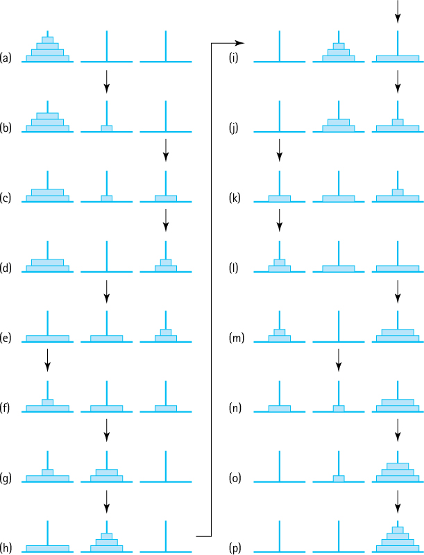
Figure 3.3 Towers of Hanoi solution for four rings

This allows us to move the largest ring from peg 1 to peg 3.

Can you see why at this point we are halfway to our completed solution? What remains is to move the three smallest rings from peg 2 to peg 3, using peg 1 as an auxiliary peg. This task is achieved by the seven moves represented by Figures 3.3i through 3.3p. These seven moves are essentially the same moves made in the first seven steps, albeit with different starting, ending, and auxiliary pegs (compare the patterns of the small arrows to verify this statement). Those last seven moves are summarized here.

We solve the puzzle for four rings by first moving three rings from peg 1 to peg 2, then moving the largest ring from peg 1 to peg 3, and finally by moving three rings (again) from peg 2 to peg 3. Aha! We solve the puzzle for four rings by solving the puzzle for three rings—in fact by solving the puzzle for three rings twice.
It is this insight, the recognition of a solution to the problem that uses solutions to smaller versions of the problem, that leads us to our recursive solution. We can solve the general problem for n rings the same way. The general recursive algorithm for moving n rings from the starting peg to the destination peg is as follows.
The Method
Let us write a recursive method that implements this algorithm. We can see that recursion works well because the first and third steps of the algorithm essentially repeat the overall algorithm, albeit with a smaller number of rings. Notice, however, that the starting peg, the destination peg, and the auxiliary peg are different for the subproblems; they keep changing during the recursive execution of the algorithm. To make the method easier to follow, the pegs are called startPeg, endPeg, and auxPeg. These three pegs, along with the number of rings on the starting peg, are the parameters of the method. The program will not actually move any rings but it will print out a message describing the moves.
Our algorithm explicitly defines the recursive or general case, but what about a base case? How do we know when to stop the recursive process? The key is to note that if there is only one ring to move we can just move it; there are no smaller disks to worry about. Therefore, when the number of rings equals 1, we simply print the move. That is the base case. The method assumes the arguments passed are valid.
public static void doTowers(
       int n,           // Number of rings to move
       int startPeg,    // Peg containing rings to move
       int auxPeg,      // Peg holding rings temporarily
       int endPeg)      // Peg receiving rings being moved

{
   if (n == 1) // Base case – Move one ring
      System.out.println("Move ring " + n + " from peg " + startPeg
                          + " to peg " + endPeg);
   else
   {
      // Move n - 1 rings from starting peg to auxiliary peg
      doTowers(n - 1, startPeg, endPeg, auxPeg);
      // Move nth ring from starting peg to ending peg
      System.out.println("Move ring " + n + " from peg " + startPeg
                          + " to peg " + endPeg);
      // Move n - 1 rings from auxiliary peg to ending peg
      doTowers(n - 1, auxPeg, startPeg, endPeg);
   }
}
It is hard to believe that such a simple method actually works, but it does. Let us investigate using the Three-Question Approach:
The Base-Case Question Is there a nonrecursive way out of the method, and does the method work correctly for this base case? If the
doTowersmethod is passed an argument equal to 1 for the number of rings (parametern), it prints the move, correctly recording the movement of a single ring fromstartPegtoendPeg,and skips the body of the else statement. No recursive calls are made. This response is appropriate because there is only one ring to move and no smaller rings to worry about. The answer to the base-case question is yes.The Smaller-Caller Question Does each recursive call to the method involve a smaller case of the original problem, leading inescapably to the base case? The answer is yes, because the method receives a ring count argument
nand in its recursive calls passes the ring count argumentn - 1. The subsequent recursive calls also pass a decremented value of the argument, until finally the value sent is 1.The General-Case Question Assuming the recursive calls work correctly, does the method work in the general case? The answer is yes. Our goal is to move n rings from the starting peg to the ending peg. The first recursive call within the method moves n – 1 rings from the starting peg to the auxiliary peg. Assuming that operation works correctly, we now have one ring left on the starting peg and the ending peg is empty. That ring must be the largest, because all of the other rings were on top of it. We can move that ring directly from the starting peg to the ending peg, as described in the output statement. The second recursive call now moves the n – 1 rings that are on the auxiliary peg to the ending peg, placing them on top of the largest ring that was just moved. As we assume this transfer works correctly, we now have all n rings on the ending peg.
We have answered all three questions affirmatively.
The Program
We enclose the doTowers method within a driver class called Towers. It prompts the user for the number of rings and then uses doTowers to report the solution. Our program ensures that doTowers is called with a positive integral argument. The Towers application can be found in the ch03.apps package. Here is the output from a run with four rings:
Input the number of rings: 4
Towers of Hanoi with 4 rings
Move ring 1 from peg 1 to peg 2
Move ring 2 from peg 1 to peg 3
Move ring 1 from peg 2 to peg 3
Move ring 3 from peg 1 to peg 2
Move ring 1 from peg 3 to peg 1
Move ring 2 from peg 3 to peg 2
Move ring 1 from peg 1 to peg 2
Move ring 4 from peg 1 to peg 3
Move ring 1 from peg 2 to peg 3
Move ring 2 from peg 2 to peg 1
Move ring 1 from peg 3 to peg 1
Move ring 3 from peg 2 to peg 3
Move ring 1 from peg 1 to peg 2
Move ring 2 from peg 1 to peg 3
Move ring 1 from peg 2 to peg 3
Try the program for yourself. But be careful—with two recursive calls within the doTowers method, the amount of output generated by the program grows quickly. In fact, every time you add one more ring to the starting peg, you more than double the amount of output from the program. A run of Towers on the author’s system, with an input argument indicating 16 rings, generated a 10-megabyte output file.
3.6 Fractals
As discussed in the “Generating Images” boxed feature in Chapter 1, digitized images can be viewed as two dimensional arrays of picture elements called pixels. In this section we investigate an approach to generating interesting, beautiful images with a simple recursive program.
There are many different ways that people define the term “fractal.” Mathematicians study continuous but not differentiable functions, scientists notice patterns in nature that repeat certain statistical measurements within themselves, and engineers create hierarchical self-similar structures. For our purposes we define a fractal as an image that is composed of smaller versions of itself. Using recursion it is easy to generate interesting and eye-pleasing fractal images.
A T-Square Fractal
In the center of a square black canvas we draw a white square, one-quarter the size of the canvas (see Figure 3.4a). We then draw four more squares, each centered at a corner of the original white square, each one-quarter the size of the original white square, that is, one-eighth the size of the canvas (see Figure 3.4b). For each of these new squares we do the same, drawing four squares of smaller size at each of their corners (see Figure 3.4c). And again (see Figure 3.4d). We continue this recursive drawing scheme, drawing smaller and smaller squares, until we can no longer draw any more squares, that is until our integer division gives a result of zero (see Figure 3.4e and a larger version in Figure 3.5a). Theoretically, using real number division, we could continue dividing the size of the squares by four forever. This is why people sometimes view fractals as infinitely recursive.
Our resulting image is a fractal called a T-square because within it we can see shapes that remind us of the technical drawing instrument of the same name. The approach used to create the T-square is similar to approaches used to create some better-known fractals, specifically the Koch snowflake and Sierpinski triangle, both based on recursively drawing equilateral triangles and the Sierpinski carpet, which is also based on recursively drawing squares but features eight squares drawn along the border of the original square.
The following program creates a 1,000 × 1,000 pixel jpg file containing a T-square fractal image. The name of the file to hold the generated image is provided as a command line argument. The program first “paints” the entire image black and then calls the recursive drawSquare method, passing it the coordinates of the “first” square and the length of a side. The drawSquare method computes the corners of the square, “paints” the square white, and then recursively calls itself, passing as arguments the coordinates of its four corners and the required smaller side dimension. This calling pattern repeats over and over until the base case is reached. The base case occurs when the size of the side of the square to be drawn is 0. The visual result of running the program can be seen in Figure 3.5a.

Figure 3.4 Stages of drawing a T-square

Figure 3.5 Samples of variations on the T-square application
//*********************************************************************
// TSquare.java              By Dale/Joyce/Weems              Chapter 3
//
// Creates a jpg file containing a recursive TSquare.
// Run argument 1: full name of target jpg file
//
//********************************************************************
package ch03.fractals;

import java.awt.image.*;     import java.awt.Color;
import java.io.*;            import javax.imageio.*;

public class TSquare
{
   static final int SIDE = 1000;     // image is SIDE X SIDE
   static BufferedImage image =
          new BufferedImage(SIDE, SIDE, BufferedImage.TYPE_INT_RGB);
   static final int WHITE = Color.WHITE.getRGB();
   static final int BLACK = Color.BLACK.getRGB();

   private static void drawSquare(int x, int y, int s)
   // center of square is x,y length of side is s
   {
      if (s <= 0) // base case
         return;
      else
      {
         // determine corners
         int left = x - s/2;     int right = x + s/2;
         int top = y - s/2;       int bottom = y + s/2;

         // paint the white square
         for (int i = left; i < right; i++)
            for (int j = top; j < bottom; j++)
             {
                image.setRGB(i, j, WHITE);
             }

         // recursively paint squares at the corners
         drawSquare(left, top, s/2);
         drawSquare(left, bottom, s/2);
         drawSquare(right, top, s/2);
         drawSquare(right, bottom, s/2);
      }
   }
   public static void main (String[] args) throws IOException
   {
      String fileOut = args[0];

      // make image black
      for (int i = 0; i < SIDE; i++)
         for (int j = 0; j < SIDE; j++)
         {
            image.setRGB(i, j, BLACK);
         }

      // first square
      drawSquare(SIDE/2, SIDE/2, SIDE/2);

      // save image
      File outputfile = new File(fileOut);
      ImageIO.write(image, "jpg", outputfile);
   }
}
Variations
By slightly modifying our TSquare.java program we can generate additional interesting images. Figure 3.5 shows some examples generated by the program variations described below. Part (a) of the figure shows the output from the original TSquare program. Note that all of the applications in this section are found in the ch03.fractals package.
The TSquareThreshold.java application allows the user to supply two additional arguments, both of type int, that indicate when to start and when to stop drawing squares. The first int argument indicates an inner threshold—if drawSqaure is invoked with a side value less than or equal to this threshold then it does nothing. For this program the base case occurs when we reach a square with a side less than or equal to this inner threshold value, rather than a base case of 0. The second int argument provides an outer threshold. Squares whose sides are greater than or equal to this threshold are also not drawn—although the recursive calls to drawSquare at their four corners are still executed. Suppressing the drawing of the larger squares allows more of the finer low-level details of the fractal image to appear. Simple if statements within the drawSquare method provide this additional functionality. Figure 3.5(b) shows the output from TSquareThreshold with arguments 10, 500 while part (c) shows the output with arguments 1, 80.
Considerations of printing costs preclude us from experimenting here with different colors (although some of the exercises point you in that direction). We can, however, play with gray levels as we did in the “Generating Images” boxed feature in Chapter 1. As explained in that feature, within the RGB color model, colors with identical red, green, and blue values are “gray.” For example, (0, 0, 0) represents black, (255, 255, 255) represents white, and (127, 127, 127) represents a medium gray. The TSquareGray.java program takes advantage of this balanced approach to “grayness” to use different gray scale levels when drawing each set of differently sized squares. A while loop in the main method calculates the number of levels needed and sets the variable grayDecrement appropriately— so that the widest range of gray possible is used within the fractal. A gray scale parameter is included for the recursive drawSquare method. It is originally passed an argument indicating white, and each time a new level of squares to be drawn is reached, the value is decremented before the recursive calls to draw the four smaller squares are executed. Figure 3.5(d) shows the output from TSquareGray with command line arguments 10, 500. The same arguments were used to generate the completely black and white image in part (b) of the figure directly above it. Can you see how the two figures are related?
3.7 Removing Recursion
Some languages do not support recursion. Sometimes, even when a language does support recursion, a recursive solution is not desired because it is too costly in terms of space or time. This section considers two general techniques that are often used to replace recursion: eliminating tail recursion and direct use of a stack. First it looks at how recursion is implemented. Understanding how recursion works helps us see how to develop nonrecursive solutions.
How Recursion Works
The translation of high-level programs into machine language is a complex process. To facilitate our study of recursion, we make several simplifying assumptions about this process. Furthermore, we use a simple program, called Kids, that is not object-oriented; nor is it a good example of program design. It does provide a useful example for the current discussion, however.
Static Storage Allocation
A compiler that translates a high-level language program into machine code for execution on a computer must perform two functions:
Reserve space for the program variables.
Translate the high-level executable statements into equivalent machine language statements.
Typically, a compiler performs these tasks modularly for separate program subunits. Consider the following program.
package ch03.apps;
public class Kids
{
   private static int countKids(int girlCount, int boyCount)
   {
       int totalKids;
       totalKids = girlCount + boyCount;
       return(totalKids);
   }
   public static void main(String[] args)
   {
       int numGirls;
       int numBoys;
       int numChildren;
       numGirls = 12;
       numBoys = 13;
       numChildren = countKids(numGirls, numBoys);
       System.out.println("Number of children is " + numChildren);
   }
}
A compiler could create two separate machine code units for this program: one for the countKids method and one for the main method. Each unit would include space for its variables plus the sequence of machine language statements that implement its high-level code.
In our simple Kids program, the only invocation of the countKids method is from the main program. The flow of control of the program is

The compiler might arrange the machine code that corresponds to the Kids program in memory something like this:
Static allocation like this is the simplest approach possible. But it does not support recursion. Do you see why?
The space for the countKids method is assigned to it at compile time. This strategy works well when the method will be called once and then always return, before it is called again. But a recursive method may be called again and again before it returns. Where do the second and subsequent calls find space for their parameters and local variables? Each call requires space to hold its own values. This space cannot be allocated statistically because the number of calls is unknown at compile time. A language that uses only static storage allocation cannot support recursion.
Dynamic Storage Allocation
Dynamic storage allocation provides memory space for a method when it is called. Local variables are thus not associated with actual memory addresses until run time.
Let us look at a simplified version of how this approach might work in Java. (The actual implementation depends on the particular system.) When a method is invoked, it needs space to keep its parameters, its local variables, and the return address (the address in the calling code to which the computer returns when the method completes its execution). This space is called an activation record or stack frame. Consider our recursive factorial method:
public static int factorial(int n)
{
   if (n == 0)
       return 1;     // Base case
   else
       return (n * factorial(n - 1));     // General case
}
A simplified version of an activation record for method factorial might have the following “declaration”:
class ActivationRecordType
{
   AddressType returnAddr;               // Return address
   int result;                           // Returned value
   int n;                                // Parameter
}
Each call to a method, including recursive calls, causes the Java run-time system to allocate additional memory space for a new activation record. Within the method, references to the parameters and local variables use the values in the activation record. When the method ends, the activation record space is released.
What happens to the activation record of one method when a second method is invoked? Consider a program whose main method calls proc1, which then calls proc2. When the program begins executing, the “main” activation record is generated (the main method’s activation record exists for the entire execution of the program).

At the first method call, an activation record is generated for proc1.

When proc2 is called from within proc1, its activation record is generated. Because proc1 has not finished executing, its activation record is still around. Just like the index cards we used in Section 3.1, “Recursive Definitions, Algorithms, and Programs,” the activation record is stored until needed:

When proc2 finishes executing, its activation record is released. But which of the other two activation records becomes the active one: proc1’s or main’s? You can see that proc1’s activation record should now be active. The order of activation follows the last in, first out (LIFO) rule. We know of a structure that supports LIFO access—the stack—so it should come as no surprise that the structure that keeps track of activation records at run time is called the run-time or system stack.
When a method is invoked, its activation record is pushed onto the run-time stack. Each nested level of method invocation adds another activation record to the stack. As each method completes its execution, its activation record is popped from the stack. Recursive method calls, like calls to any other method, cause a new activation record to be generated.
The number of recursive calls that a method goes through before returning determines how many of its activation records appear on the run-time stack. The number of these calls is the depth of the recursion.
Now that we have an understanding of how recursion works, we turn to the primary topic of this section: how to develop nonrecursive solutions to problems based on recursive solutions.
Tail Call Elimination
When the recursive call is the last action executed in a recursive method, an interesting situation occurs. The recursive call causes an activation record to be put on the run-time stack; this record will contain the invoked method’s arguments and local variables. When the recursive call finishes executing, the run-time stack is popped and the previous values of the variables are restored. Execution continues where it left off before the recursive call was made. Because the recursive call is the last statement in the method, however, there is nothing more to execute, and the method terminates without using the restored local variable values. The local variables did not need to be saved. Only the arguments in the call and its return value are actually significant.
In such a case we do not really need recursion. The sequence of recursive calls can be replaced by a loop structure. For instance, for the factorial method presented in Section 3.1, “Recursive Definitions, Algorithms, and Programs,” the recursive call is the last statement in the method:
public static int factorial(int n)
{
   if (n == 0)
       return 1;      // Base case
   else
       return (n * factorial(n - 1));    // General case
}
Now we investigate how we could move from the recursive version to an iterative version using a while loop.
For the iterative solution we need to declare a variable to hold the intermediate values of our computation. We call it retValue, because eventually it holds the final value to be returned.
A look at the base case of the recursive solution shows us the initial value to assign to retValue. We must initialize it to 1, the value that is returned in the base case. This way the iterative method works correctly in the case when the loop body is not entered.
Now we turn our attention to the body of the while loop. Each time through the loop should correspond to the computation performed by one recursive call. Therefore, we multiply our intermediate value, retValue, by the current value of the n variable. Also, we decrement the value of n by 1 each time through the loop—this action corresponds to the smaller-caller aspect of each invocation.
Finally, we need to determine the loop termination conditions. Because the recursive solution has one base case—if the n argument is 0—we have a single termination condition. We continue processing the loop as long as the base case is not met:
while (n != 0)
Putting everything together we arrive at an iterative version of the method:
private static int factorial(int n)
{
   int retValue = 1;      // return value
   while (n != 0)
   {
       retValue = retValue * n;
       n = n - 1;
   }
   return(retValue);
}
Cases in which the recursive call is the last statement executed are called tail recursion. Tail recursion always can be replaced by iteration following the approach just outlined. In fact, some optimizing compilers will remove tail recursion automatically when generating low-level code.
Direct Use of a Stack
When the recursive call is not the last action executed in a recursive method, we cannot simply substitute a loop for the recursion. For instance, consider the method recRevPrintList, which we developed in Section 3.4, “Recursive Processing of Linked Lists,” for printing a linked list in reverse order:
void recRevPrintList(LLNode<String> listRef)
// Prints the contents of the listRef linked list to standard output
// in reverse order
{
   if (listRef != null)
   {
       recRevPrintList(listRef.getLink());
       System.out.println(listRef.getInfo());
   }
}
Here we make the recursive call and then print the value in the current node. In cases like this one, to remove recursion we can replace the stacking of activation records that is done by the system with stacking of intermediate values that is done by the program.
For our reverse printing example, we must traverse the list in a forward direction, saving the information from each node onto a stack, until reaching the end of the list (when our current reference equals null). Upon reaching the end of the list, we print the information from the last node. Then, using the information we saved on the stack, we back up (pop) and print again, back up and print, and so on, until we have printed the information from the first list element.
Here is the code:
static void iterRevPrintList(LLNode<String> listRef)
// Prints the contents of the listRef linked list to standard output
// in reverse order
{
   StackInterface<String> stack = new LinkedStack<String>();
   while (listRef != null) // put info onto the stack
   {
      stack.push(listRef.getInfo());
      listRef = listRef.getLink();
   }
   // Retrieve references in reverse order and print elements
   while (!stack.isEmpty())
   {
      System.out.println(stack.top());
      stack.pop();
   }
}
Notice that the programmer stack version of the reverse print operation is quite a bit longer than its recursive counterpart, especially if we add in the code for the stack methods push, pop, top, and isEmpty. This extra length is caused by our need to stack and unstack the information explicitly. Knowing that recursion uses the system stack, we can see that the recursive algorithm for reverse printing is also using a stack—an invisible stack that is automatically supplied by the system. That is the secret to the elegance of recursive-problem solutions.
The reverse print methods presented in this section are included in the cho3.apps package in the file LinkedListReverse.java. The application includes both the recursive and iterative reverse print methods plus test code that exercises each of the methods on lists of size 0, 1, and 5.
3.8 When to Use a Recursive Solution
We might consider several factors when deciding whether to use a recursive solution to a problem. The main issues are the efficiency and the clarity of the solution.
Recursion Overhead
A recursive solution is often more costly in terms of both computer time and space than a nonrecursive solution. (This is not always the case; it really depends on the problem, the computer, and the compiler.) A recursive solution usually requires more “overhead” because of the nested recursive method calls, in terms of both time (each call involves processing to create and dispose of the activation record and to manage the run-time stack) and space (activation records must be stored). Calling a recursive method may generate many layers of recursive calls. For instance, the call to an iterative solution to the factorial problem involves a single method invocation, causing one activation record to be put on the run-time stack. Invoking the recursive version of factorial requires n + 1 method calls and pushes n + 1 activation records onto the run-time stack. That is, the depth of recursion is O(n). Besides the obvious run-time overhead of creating and removing activation records, for some problems the system just may not have enough space in the run-time stack to run a recursive solution.
Inefficient Algorithms
Another potential problem is that a particular recursive solution might just be inherently inefficient. Such inefficiency is not a reflection of how we choose to implement the algorithm; rather, it is an indictment of the algorithm itself.
Combinations
Consider the problem of determining how many combinations of a certain size can be made out of a group of items. For instance, if we have a group of 20 students and want to form a panel (subgroup) consisting of five student members, how many different panels are possible?
A recursive mathematical formula can be used for solving this problem. Given that C is the total number of combinations, group is the total size of the group to pick from, members is the size of each subgroup, and group > members,

The reasoning behind this formula is as follows:
The number of ways you can select a single member of a group (a subgroup of size 1) is equal to the size of the group (you choose the members of the group one at a time).
The number of ways you can create a subgroup the same size as the original group is 1 (you choose everybody in the group).
If neither of the aforementioned situations apply then you have a situation where each member of the original group will be in some subgroups but not in other subgroups; the combination of the subgroups that a member belongs to and the subgroups that member does not belong to represents all of the subgroups; therefore, identify a member of the original group randomly and add together the number of subgroups to which that member belongs [C(group - 1, members - 1)] (our identified member belongs to the subgroup but we still need to choose members – 1 members from the remaining group – 1 possibilities) and the number of subgroups that member does not belong too [C(group - 1, members)] (we remove the identified member from consideration).
Because this definition of C is recursive, it is easy to see how a recursive method can be used to solve the problem.
public static int combinations(int group, int members)
{
   if (members == 1)
       return group;               // Base case 1
   else if (members == group)
       return 1;                   // Base case 2
   else
       return (combinations(group - 1, members - 1) +
          combinations(group - 1, members));
}
The recursive calls for this method, given initial arguments (4, 3), are shown in Figure 3.6.
Returning to our original problem, we can now find out how many panels of five student members can be made from the original group of 20 students with the statement
System.out.println("Combinations = " + combinations(20, 5));

Figure 3.6 Calculating combinations(4,3)
that outputs “Combinations = 15504.” Did you guess that it would be that large of a number? Recursive definitions can be used to define functions that grow quickly!
Although it may appear elegant, this approach to calculating the number of combinations is extremely inefficient. The example of this method illustrated in Figure 3.6, combinations(4,3), seems straightforward enough. But consider the execution of combinations(6,4), as illustrated in Figure 3.7. The inherent problem with this method is that the same values are calculated over and over. For example, combinations(4,3) is calculated in two different places, and combinations(3,2) is calculated in three places, as are combinations(2,1) and combinations(2,2).
It is unlikely that we could solve a combinatorial problem of any large size using this method. For large problems the program runs “forever”—or until it exhausts the capacity of the computer; it is an exponential-time, O(2N), solution to the problem.
Although our recursive method is very easy to understand, it is not a practical solution. In such cases, you should seek an alternative solution. A programming approach called dynamic programming, where solutions to subproblems that are needed repeatedly are saved in a data structure instead of being recalculated, can often prove useful. Or, even better, you might discover an efficient iterative solution. For the combinations problem an easy (and efficient) iterative solution does exist, as mathematicians can provide us with another definition of the function C:
C (group, members) = group!/((members!) × (group – members)!)
A carefully constructed iterative program based on this formula is much more efficient than our recursive solution.
Clarity
The issue of the clarity of a problem solution is also an important factor in determining whether to use a recursive approach. For many problems, a recursive solution is simpler and more natural for the programmer to write. The total amount of work required to solve a problem can be envisioned as an iceberg. By using recursive programming, the application programmer may limit his or her view to the tip of the iceberg. The system takes care of the great bulk of the work below the surface.
Compare, for example, the recursive and nonrecursive approaches to printing a linked list in reverse order that were developed earlier in this chapter. In the recursive version, the system took care of the stacking that we had to do explicitly in the nonrecursive method. Thus, recursion is a tool that can help reduce the complexity of a program by hiding some of the implementation details. With the cost of computer time and memory decreasing and the cost of a programmer’s time rising, it is worthwhile to use recursive solutions to such problems.

Figure 3.7 Calculating combinations(6,4)
Summary
Recursion is a very powerful problem-solving technique. Used appropriately, it can simplify the solution of a problem, often resulting in shorter, more easily understood source code. As usual in computing, trade-offs become necessary: Recursive methods are often less efficient in terms of both time and space, due to the overhead of many levels of method calls. The magnitude of this cost depends on the problem, the computer system, and the compiler.
A recursive solution to a problem must have at least one base case—that is, a case in which the solution is derived nonrecursively. Without a base case, the method recurses forever (or at least until the computer runs out of memory). The recursive solution also has one or more general cases that include recursive calls to the method. These recursive calls must involve a “smaller caller.” One (or more) of the argument values must change in each recursive call to redefine the problem to be smaller than it was on the previous call. Thus, each recursive call leads the solution of the problem toward the base case.
Many data structures, notably trees but even simpler structures such as arrays and linked lists, can be treated recursively. Recursive definitions, algorithms, and programs are a key part of the study of data structures.
Exercises
Basics (Sections 3.1 and 3.2)
Exercises 1 to 3 use the following three mathematical functions (assume N ≥ 0):
Sum(N) = 1 + 2 + 3 + . . . + N
BiPower(N) = 2N
TimesFive(N) = 5N
-
Define recursively
Sum(N)
BiPower(N)
TimesFive(N)
-
 Create a recursive program that prompts the user for a nonnegative integer N and outputs.
Sum(N)
BiPower(N)
TimesFive(N)
Describe any input constraints in the opening comment of your recursive methods.
-
Use the Three-Question Approach to verify the program(s) you created for Exercise 2. Exercises 4 to 5 use the following method:
int puzzle(int base, int limit) { if (base > limit) return -1; else if (base == limit) return 1; else return base * puzzle(base + 1, limit); } -
Identify
The base case(s) of the
puzzlemethodThe general case(s) of the
puzzlemethodConstraints on the arguments passed to the
puzzlemethod
-
Show what would be written by the following calls to the recursive method
puzzle.System.out.println(puzzle (14, 10));System.out.println(puzzle (4, 7));System.out.println(puzzle (0, 0));
-
Given the following method:
int exer(int num)
{
   if (num == 0)
      return 0;
   else
      return num + exer(num + 1);
}
Is there a constraint on the value that can be passed as an argument for this method to pass the smaller-caller test?
Is
exer(7)a valid call? If so, what is returned from the method?Is
exer(0)a valid call? If so, what is returned from the method?Is
exer(-5)a valid call? If so, what is returned from the method?
-
For each of the following recursive methods, identify the base case, the general case, and the constraints on the argument values, and explain what the method does.
int power(int base, int exponent)
{
if (exponent == 0)
   return 1;

else
   return (base * power(base, exponent-1));
}
int factorial (int n) { if (n > 0) return (n * factorial (n - 1)); else if (n == 0) return 1; }int recur(int n) { if (n < 0) return -1; else if (n < 10) return 1; else return (1 + recur(n / 10)); }int recur2(int n) { if (n < 0) return -1; else if (n < 10) return n; else return ((n % 10) + recur2(n / 10)); }
-
 Code the methods described in parts a and b. Hint: Use recursion to iterate across the lines of asterisks, but use a for loop to generate the asterisks within a line.
Code a recursive method
printTriangleUp(int n)that prints asterisks toSystem.outconsisting ofnlines, with one asterisk on the first line, two on the second line, and so on. For example, ifnis 4 the final result would be:* ** *** ****
Code a recursive method
printTriangleDn(int n)that prints asterisks toSystem.outconsisting ofnlines, withnasterisk on the first line,n-1on the second line, and so on. For example, ifnis 4 the final result would be:**** *** ** *
-
The greatest common divisor of two positive integers m and n, referred to as gcd(m, n), is the largest divisor common to m and n. For example, gcd(24, 36) = 12, as the divisors common to 24 and 36 are 1, 2, 3, 4, 6, and 12. An efficient approach to calculating the gcd, attributed to the famous ancient Greek mathematician Euclid, is based on the following recursive algorithm:
Design, implement, and test a program
Euclidthat repeatedly prompts the user for a pair of positive integers and reports the gcd of the entered pair. Your program should use a recursive methodgcdbased on the above algorithm.
3.3 Recursive Processing of Arrays
-
The sorted values array contains 16 integers 5, 7, 10, 13, 13, 20, 21, 25, 30, 32, 40, 45, 50, 52, 57, 60.
Indicate the sequence of recursive calls that are made to
binarySearch, given an initial invocation ofbinarySearch(32,0,15).Indicate the sequence of recursive calls that are made to
binarySearch, given an initial invocation ofbinarySearch(21,0,15).Indicate the sequence of recursive calls that are made to
binarySearch, given an initial invocation ofbinarySearch(42,0,15).Indicate the sequence of recursive calls that are made to
binarySearch, given an initial invocation ofbinarySearch(70,0,15).
-
You must assign the grades for a programming class. Right now the class is studying recursion, and students have been given this assignment: Write a recursive method
sumValuesthat is passed an index into an array values ofint(this array is accessible from within thesumValuesmethod) and returns the sum of the values in the array between the location indicated byindexand the end of the array. The argument will be between 0 andvalues.lengthinclusive. For example, given this configuration:
then
sumValues(4)returns 12 andsumValues(0)returns 34 (the sum of all the values in the array). You have received quite a variety of solutions. Grade the methods below. If the solution is incorrect, explain what the code actually does in lieu of returning the correct result. You can assume the array is “full.” You can assume a “friendly” user—the method is invoked with an argument between 0 andvalues.length.int sumValues(int index) { if (index == values.length) return 0; else return index + sumValues(index + 1); }int sumValues(int index) { int sum = 0; for (int i = index; i < values.length; i++) sum = sum + values[i]; return sum; }int sumValues(int index) { if (index == values.length) return 0; else return (1 + sumValues(index + 1); }int sumValues(int index) { return values[index] + sumValues(index + 1); }int sumValues(int index) { if (index > values.length) return 0; else return values[index] + sumValues(index + 1); }int sumValues(int index) { if (index >= values.length) return 0; else return values[index] + sumValues(index + 1); }int sumValues(int index) { if (index < 0) return 0; else return values[index] + sumValues(index - 1); }
-
Assume we have an unsorted array of
intnamedvaluesthat is accessible from within the recursive methodsmallestValue. Our specific problem is to determine the smallest element of the array. Our approach is to use the fact that the smallest element in a subarray is equal to the smaller of the first element in the subarray and the smallest element in the remainder of the subarray. The subarrays we examine will always conclude at the end of the overall array; therefore we only need to pass our recursive method a single parameter, indicating the start of the subarray currently being examined. The signature for the method isint smallestValue(int first)
For example, given the values array from Exercise 11,
smallestValue(4)returns 3 andsmallestValue(0)returns 2 (the smallest value in the array). Design and code the recursive methodsmallestValueplus a test driver. -
Consider that we can define the reverse of a string
srecursively as:
Create an application that prompts the user for a string, then outputs the string in reverse. For example, if the user inputs “abcd efg,” then your application should output “gfe dcba.” Within your application include a static recursive method
reversebased on the above definition, that takes aStringargument and returns aStringthat is the reverse of the argument.Show the sequence of method calls to
reversethat your application makes if the user inputs “RECURSE.”
3.4 Recursive Processing of Linked Lists
-
This exercise uses the methods
recPrintList,recListSize, andrecRevPrintListdefined in Section 3.4. Assumelistis of typeLLNode<String>and points to the start of a linked list containing the following strings, in the order shown:alpha beta comma delta emma. For each of the following, indicate the sequence of recursive calls that results from the initial call shown. Include in your answer an indication of the information in theLLNodethat is the argument of the call, for example, “recPrintList(pointer to node containing delta).”Initial call is
recPrintList(list)(in other wordsrecPrintList(pointer to node containing alpha)).Initial call is
recListSize(list)(in other wordsrecListSize(pointer to node containing alpha)).Initial call is
recRevPrintList(list)(in other wordsrecRevPrintList(pointer to node containing alpha)).
-
You must assign the grades for a programming class. Right now the class is studying recursion, and students have been given this assignment: Write a recursive method
sumSquaresthat is passed a reference to a linked list ofIntegerelements and returns the sum of the squares of the elements. The list nodes are of classLLNode<Integer>. The objects in the list are all of classInteger. Example:
Assume that the list is not empty. You have received quite a variety of solutions. Grade the methods below, marking errors where you see them.
int sumSquares(LLNode<Integer> list)
{
   return 0;
   if (list != null)
    return (list.getInfo()* list.getInfo()+
   sumSquares(list.getLink()));
}
int sumSquares(LLNode<Integer> list) { int sum = 0; while (list != null) { sum = list.getInfo() + sum; list = list.getLink(); } return sum; }int sumSquares(LLNode<Integer> list) { if (list == null) return 0; else return list.getInfo() * list.getInfo() + sumSquares(list.getLink()); }int sumSquares(LLNode<Integer> list) { if (list.getLink() == null) return list.getInfo() * list.getInfo(); else return list.getInfo() * list.getInfo() + sumSquares(list.getLink()); }int sumSquares(LLNode<Integer> list) { if (list == null) return 0; else return (sumSquares(list.getLink()) * sumSquares(list.getLink())); }
For exercises 16 to 19 assume we have a sorted linked list of
Integer. The start of the linked list is referenced byvalueswhich, of course, is of typeLLNode<Integer>. For example purposes, assumevaluespoints to a list containing 3, 6, 6, 9, 12, 15, 18, 19, 19, and 20. You can and should assume the list in question is sorted in nondecreasing order. For each of these exercises you should also create a driver application that demonstrates that your new method operates correctly. -
Write a recursive method
numEvens(LLNode<Integer> list)that returns how many even numbers are contained inlist. For our example listnumEvens(values)would return 5 (the even numbers are 6, 6, 12, 18, and 20). -
Write a recursive method
contains(int target, LLNode<Integer> list)that returnstrueiflistcontainstargetandfalseotherwise. For our example listcontains(15, values)would return true whilecontains(10, values)would returnfalse. -
Write a recursive method
remove(int target, LLNode<Integer> list)that removes all occurrences oftargetfromlistand returns a reference to the new list. For our example list the statementvalues = remove(6, values);
would result in
valuesreferencing the list containing 3 9 12 15 18 19 19 and 20. Iftargetis not contained inlistthen the list remains unchanged. -
Write a recursive method
insertOrdered(int target, LLNode<Integer> list)that addstargetto the ordered linked list referenced bylist, such that the linked list remains sorted, and returns a reference to the new list. For our example list the statementvalues = insertOrdered(16, values);
would result in
valuesreferencing the list containing 3 6 6 9 12 16 18 19 19 and 20.
3.5 Towers
-
What are the constraints on the arguments for parameter
nof thedoTowersmethod? What happens if the constraints are not met? -
Change the Towers of Hanoi program so that it does the following:
Counts the number of ring moves and prints that out instead of the sequence of moves. Use a static variable
countof typeintto hold the number of moves.Repeatedly prompts the user for the number of rings and reports the results, until the user enters a number less than 0.
-
Using your version of the Towers of Hanoi program from Exercise 21, answer the following:
Fill in the table with the number of moves required to solve the problem, starting with the given number of rings.
Rings Moves 1 2 3 4 5 6 7 Describe the pattern you see in the number of moves listed in your table.
Assuming n > 0, define the number of moves required to move n rings using a recursive mathematical formula.
Suppose you have a physical Towers of Hanoi puzzle with 11 rings. If it takes one second to move a ring from one peg to another, how long would it take you to “solve” the puzzle?
In Java the data type
intuses 32 bits and can represent integers in the range -2,147,483,648 to 2,147,483,647. By experimenting with your program from Exercise 12, figure out the largest number of rings that the program can handle before “blowing up”—that is, before the value incountoverflows.What is the number of moves reported for that number of rings? How close is that to the maximum
intvalue? Explain.In the legend described on page xxx the monks are solving a tower that has 64 rings. How many moves are required? At the rate of one move per second, how long will it take for the monks to complete the puzzle (and end the world!)?
-
Towers of Hanoi Variation: In this new version of the Towers of Hanoi puzzle we add the additional constraint that every move must use the middle peg. For example, if the pegs are labeled 1, 2, and 3 left to right and we start with two rings, 1 and 2 (with 1 being the smaller ring) on peg 1, then to move the rings to peg 3 we would make the following moves: move ring 1 from peg 1 to peg 2, move ring 1 from peg 2 to peg 3, move ring 2 from peg 1 to peg 2, move ring 1 from peg 3 to peg 2, move ring 1 from peg 2 to peg 1, move ring 2 from peg 2 to peg 3, move ring 1 from peg 1 to peg 2, move ring 1 from peg 2 to peg 3. Done! Note that every move used peg 2, the middle peg.
Write a program named
TowersVariation, similar to theTowersprogram, which prompts the user for the number of rings and then prints out the sequence of moves needed to solve the Towers of Hanoi Variation problem.Revise your program so that it counts the number of ring moves and prints that out instead of the sequence of moves. Use a static variable
countof typeintto hold the number of moves. Your program should now repeatedly prompt the user for the number of rings and reports the results, until the user enters a number less than 0.Create a table that compares the number of ring moves needed when solving the standard Towers problem as compared to the number required for the variation, for 1 to 10 rings.
3.6 Fractals
-
Create an application
DiminishingSquaresthat accepts a command line integer argumentnand then outputs a “square” of asterisks of sizen×n, followed by another of size(n - 1) × (n – 1), and so on, stopping after it draws a1 × 1square. Your application should include a recursivedrawSquares(int side)method that is called once by the main method and that handles all of the output. For example, if the argument to the application is 3, the output would be:*** *** *** ** ** *
-
Three fractal drawing applications were presented in this section. Here we ask you to make some modifications to these programs. Some of the modifications require knowledge about the Java
Colorclass, which you can find on the Oracle website.Create
TSquare01by modifyingTSquareso that it only draws squares at every other level. Therefore, it draws the largest square at level one, skips drawing the four smaller squares at level two, and draws the eight even smaller squares at level three, and so on.Create
TSquare02by modifyingTSquareso that it uses two interesting colors (instead of black and white) for the background and the squares.Create
TSquare03by modifyingTSquareso that it uses a black background, red for the odd numbered levels of squares, and yellow for the even numbered levels. Feel free to experiment with different color combinations until you find one that you like.Create
TSquareGray01by modifyingTSquareGrayso that it uses a random color at each level.Create
TSquareGray02by modifyingTSquareGrayso that it uses a random color for each square.Create
TSquareGray03by modifyingTSquareGrayso that it uses a consistent color pattern. Figure out a way to vary the colors used at each level using a mathematical pattern.
-
The Sierpinski carpet is a well-known plane fractal based on recursive squares.
Using
TSquare.javaas a guide, create an application calledSierpinskiCarpet.java. For this fractal imagine dividing the original square canvas into nine congruent squares, essentially creating a3 × 3grid of smaller squares. Fill in the central square. Recursively repeat the dividing and filling in on each of the outer eight squares.Experiment with shades of gray and colors as described in the previous problem.
-
Design your own image generation program that uses some type of recursion. Perhaps your class can have an Art Exhibit.
3.7 Removing Recursion
-
Explain what is meant by the following terms:
Run-time stack
Static storage allocation
Dynamic storage allocation
Activation record
Tail recursion
-
Explain the relationship between dynamic storage allocation and recursion.
-
Create an iterative version of the
Euclidprogram from Exercise 9. Call your programEuclid2. Use what you learned in this section about removing tail recursion to design your iterative approach. -
Implement a program that repeatedly asks the user to input a positive integer and outputs the factorial of that input integer. Your program should be based on our recursive solution to the factorial problem, but instead of using recursion you should use a stack.
3.8 When to Use a Recursive Solution
-
Using the
combinationsmethod from Section 3.8:Create a program that repeatedly prompts the user for two integers,
NandM, and outputs the number of combinations ofMitems that can be made out ofNitems.Enhance your program so that it also outputs the number of times the
combinationsmethod is invoked when determining each result.Experiment with your enhanced program, using different variations of input values. Write a short report about the results of your experiment.
-
The Fibonacci sequence is the series of integers
0, 1, 1, 2, 3, 5, 8, 13, 21, 34, 55, 89 . . .
See the pattern? Each element in the series is the sum of the preceding two elements. Here is a recursive formula for calculating the nth number of the sequence:

Write a recursive method
fibonaccithat returns the nth Fibonacci number when passed the argumentn.Write a nonrecursive version of the method
fibonacci.Write a driver to test your two versions of the method
fibonacci.Compare the recursive and iterative versions for efficiency. (Use words, not O( ) notation.)
Additional Problems
-
The following defines a function that calculates an approximation of the square root of a
number, starting with an approximate answer (approx), within the specified tolerance (tol).
What limitations must be placed on the values of the arguments if this function is to work correctly?
Write a recursive method
sqrRootthat implements the function.Write a nonrecursive version of the method
sqrRoot.Write a driver to test the recursive and iterative versions of the method
sqrRoot.
-
A palindrome is a string that reads the same forward as well as backward. For example, “otto” and “never odd or even” are palindromes. When determining if a string is a palindrome, we ignore characters that are not letters.
Give a recursive definition of a palindrome. (Hint: Consider what you get if you remove the first and last letters of a palindrome.)
What is the base case of your definition?
Write a recursive program based on your definition that repeatedly prompts the user for a string and then reports whether the string is a palindrome.
Write an iterative program that does the same thing.
Compare your two programs in terms of time and space efficiency.
-
Create a program that uses methods provided by the Java class library for exploring files and folders. (Hint: The
Fileclass is a good place to start.) The path to a specific file folder is provided to your program as a command line argument. Your program should do each of the following tasks:“Print” to standard output a list of all of the files in the argument folder plus their size, along with a list of any folders in the argument folder. Include for each listed folder a list of its files (including sizes) and folders. Do this “recursively” as long as there are subfolders to be listed. Your output should display the hierarchy of folders and files in a visually appealing manner.
“Print” to standard output the name, path name, and size of the largest file in the list generated in part a.
Create a report about your program that includes a program listing, sample output, and a description of your experience creating the program.
-
A Context Free Grammar (CFG) is a quadruple <V, T, P, S> where
V is a finite set of variables (nonterminals)
T is a finite set of terminal symbols
P is a finite set of productions:
A production is a rewriting rule of the form:
V → α
where V is a nonterminal, α is any string of terminals/nonterminals or the empty string,
S is a special symbol called the start symbol and is a variable
We will assume that variables are surrounded by < >, and that the empty string is represented by [ ].
A CFG can be used to generate random sentences.
We will use weighted productions where the probability that a production is used is equal to its weight divided by 100. In our list of productions we assume the sum of the weights of all productions with the same variable on the left side is 100. For example, a set of productions could be:
100 <S> = My homework is <rl> late because
<reason>.
30 <reason> = it is <rl> always late
30 <reason> = my <rl> <hungry thing> ate it
20 <hungry thing> = younger <sibling>
20 <hungry thing> = older <sibling>
50 <sibling> = brother
50 <sibling> = sister
30 <hungry thing> = dog
30 <hungry thing> = printer
10 <reason> = <reason>
and besides <rl> <reason>
20 <rl> = like
80 <rl> = []
30 <reason> = I forgot my flash drive
Sentences that could be generated based on the above set of productions include, for example:
My homework is late because      My homework is like late because
it is like always late           I forgot my flash drive
and besides my older sister ate it
List five other sentences that could be generated from the given grammar.
Design your own interesting CFG following the format shown above.
Create a program
SentenceGenthat will read a set of productions such as that shown above, and that will, at the user’s request, generate and display a random “sentence” from the grammar, until the user indicates he or she wants to quit.