13.7 Tail Recursion
13.7.1 Recursive Control Behavior
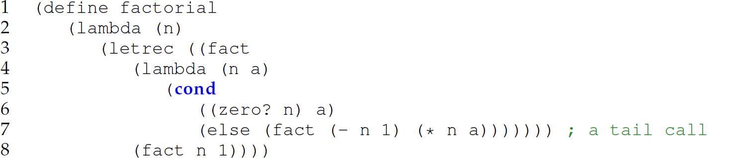
Thus far in our presentation of recursive, functional programming, we have primarily used recursive control behavior, where the definition of a recursive function naturally reflects the recursive specification of the function. For instance, consider the following definition of a factorial function in Scheme, which naturally mirrors the mathematical definition of a factorial 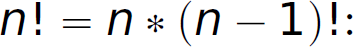
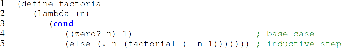
Each call to factorial is made with a promise to multiply the value returned by n at the time of the call. Examining the run-time behavior of this function with respect to the stack reveals the essence of recursive control behavior:
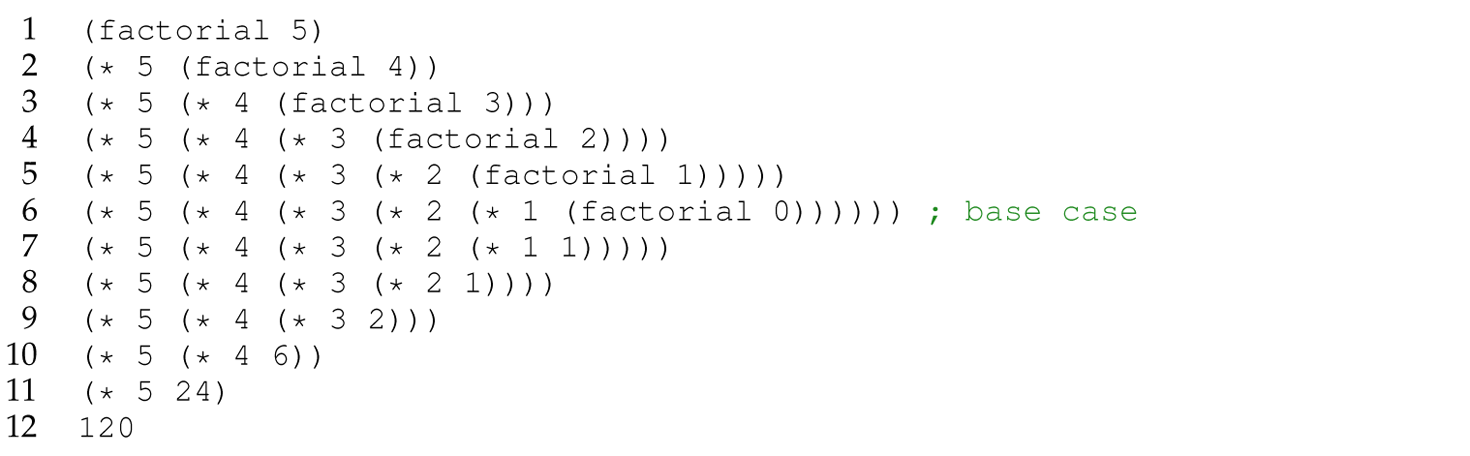
Notice how execution of this function requires an ever-increasing amount of memory (on the run-time stack) to store the control context as the depth of the recursion increases. In other words, factorial is progressively invoked in an ever larger control context as the computation proceeds. That situation occurs because the recursive call to factorial is in operand position—the return value of each recursive call to factorial becomes the second operand to the multiplication operator. The interpreter must save the context around each recursive call because it needs to remember that after the evaluation of the function invocation, the interpreter still needs to finish evaluating the operands and execute the outer call—in this case, the waiting multiplication. Thus, there is a continuation waiting for each recursive call to factorial to return. That continuation grows (lines 1–5) until the base case is reached (i.e., n = 0; line 6). The computation required to actually compute the factorial is performed as these pending multiplications execute while the activation records for the recursive calls to factorial pop off the stack (lines 7–12). Rotating the textual depiction of the control context 90 degrees to the left reveals a parabola capturing the change in the size of the stack as time proceeds during the function execution. Figure 13.7 (left) illustrates this parabola, which describes the general pattern of recursive control behavior.5 A function whose control context grows in this manner exhibits recursive control behavior. Most recursively defined functions follow this execution pattern.
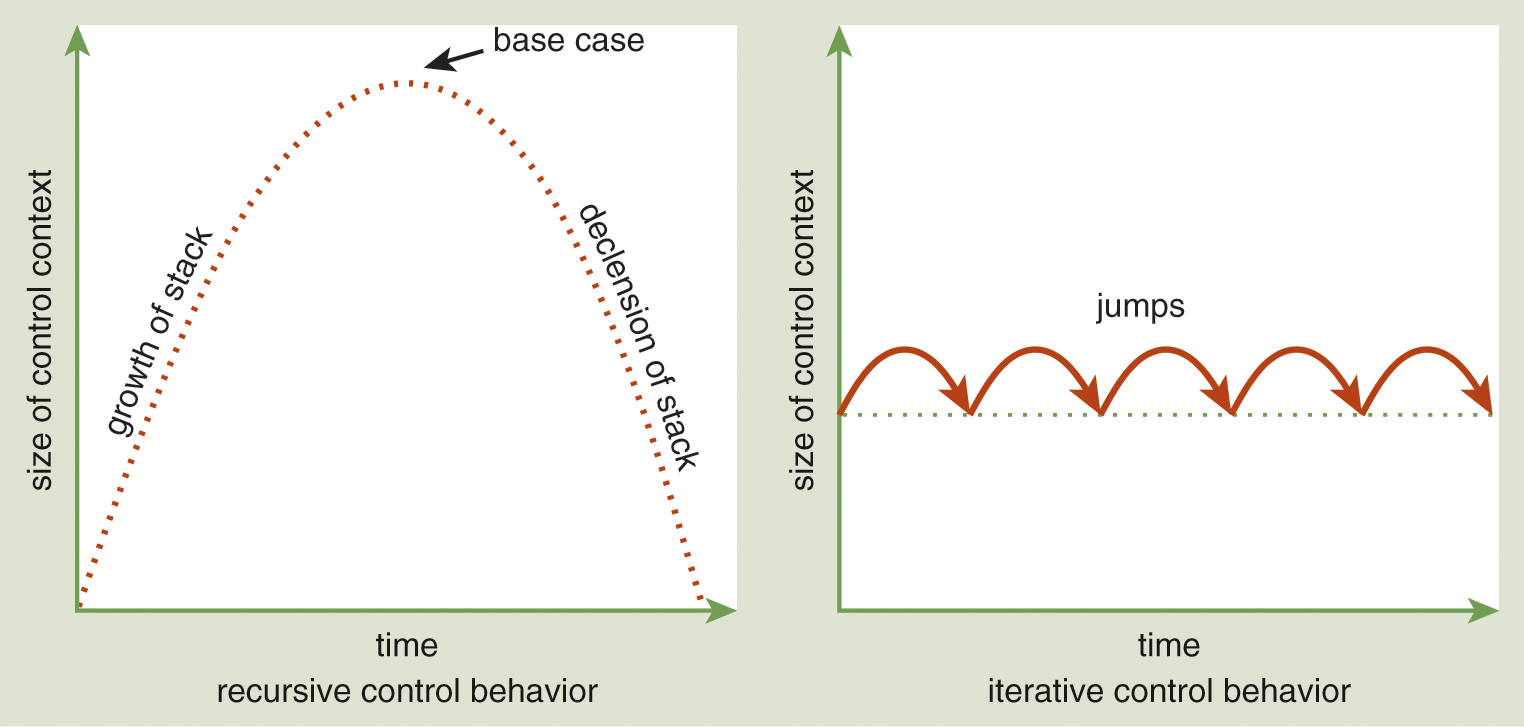
Figure 13.7 Recursive control behavior (left) vis-à-vis iterative control behavior (right).
DescriptionA key advantage of recursive control behavior is that the definition of the function reflects its specification; a disadvantage is that the amount of memory required to invoke the function is unbounded. However, we can define a recursive version of factorial that does not cause the control context to grow; in other words, this version does not require an unbounded amount of memory.
13.7.2 Iterative Control Behavior
Consider an alternative definition of a factorial function:
This version defines a nested, recursive function fact that accepts an additional parameter a, which serves as an accumulator. Unlike in the first definition, in this version of factorial, successive calls to fact do not communicate through a return value (i.e., the factorial resulting from each smaller instance of the problem). Instead, the successive recursive calls now communicate through the additional accumulator parameter.
On line 7, notice that no computation is waiting for each recursive call to fact to return; that is, the recursive call to factorial is no longer in operand position. In other words, when fact calls itself, it does so at the tail end of a call to fact. Such a recursive call is said to be in tail position—in contrast to operand position in which the recursive call to factorial is found in the first version—and referred to as a tail call. A function call is a tail call if there is no promise to do anything with the returned value. In this version of factorial, no promise is made to do anything with the return value other than return it as the result of the current call to fact. When the tail call invokes the same function in which it occurs, the approach is referred to as tail recursion. Thus, the tail call in this revised version of the factorial function uses tail recursion.
The following is a depiction of the control context of a sample execution of this new definition of factorial:
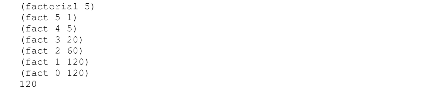
Figure 13.7 (right) illustrates this graph. Unlike with the execution pattern of the first definition of factorial, rotating this textual depiction of the control context 90 degrees to the left reveals a straight line, which indicates the control context remains constant as the function executes. That pattern is a result of iterative control behavior, where a recursive function uses a bounded control context. In this case, the function has the potential to run in constant memory space and without the use of a run-time stack because a “procedure call that does not grow control context is the same as a jump” (Friedman, Wand, and Haynes 2001, p. 262). (The strategy used to define this revised version of factorial is introduced in Section 5.6.3— through the definition of a list reverse function—as Design Guideline 7: Difference Lists Technique.)
The use of word tail in this context is slightly deceptive because it is not used in the lexicographical context of the function, but rather in the run-time context. In other words, a function that calls itself at the tail end of its definition lexicographically is not necessarily a tail call. For instance, consider line 5 in the first definition of factorial in Section 13.7.1 (repeated here):  . The recursive call to factorial in this line of code appears to be the last step of the function because it is positioned at the rightmost end of the function definition lexicographically, but it is not the final step. The key to determining whether a call is in tail or operand position is the pending continuation. If there is a continuation waiting for the recursive call to return, then the call is in operand position; otherwise, it is in tail position.
As we conclude this section, let us examine two new (tail-recursive) definitions of the product function from Section 13.3.1. The following definition is the tail-recursive version of the definition without a nonlocal exit for the exceptional case (i.e., a zero in the input list) from that section:
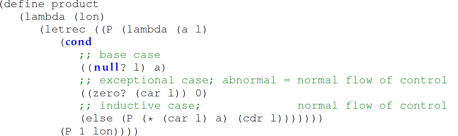
While this function is tail recursive and exhibits iterative control behavior, it may perform unnecessary multiplications if the input list contains a zero. The following definition is the tail-recursive version of the definition using a continuation captured with call/cc to perform a nonlocal exit in the exceptional case from Section 13.3.1:
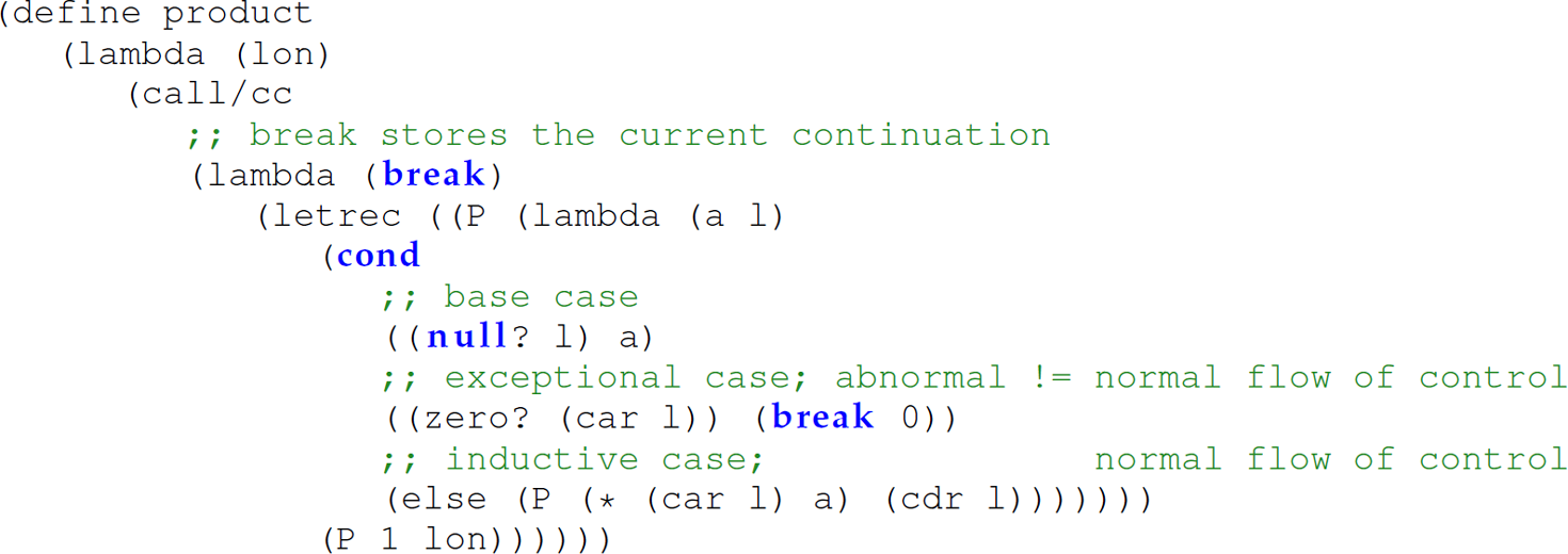
This definition, like the first one, is tail recursive, exhibits iterative control behavior, and may perform unnecessary multiplications if the input list contains a zero. However, this version avoids returning through all of the activation records built up on the call stack when a zero is encountered in the list.
13.7.3 Tail-Call Optimization
If a recursive function defined using tail recursion exhibits iterative control behavior, it has the potential to run in constant memory space. The use of tail recursion implies that no computations are waiting for the return value of each recursive call, which in turn means the function that made the recursive call can be popped off the run-time stack. However, even though tail recursion eliminates the buildup of pending computations on the run-time stack waiting to complete once the base case is reached, the activation records for each recursive tail call are still on the stack. Each activation record simply receives the return value from the function it calls and returns this value to the function that called it.
Tail-call optimization (TCO) eliminates the implicit function return in a tail call and eliminates the need for a run-time stack.6 Thus, TCO enables (recursive) functions to run in constant space—rendering recursion as efficient as iteration. The Scheme, ML, and Lua programming languages use TCO. Languages supporting functional programming can be implemented using CPS and TCO in concert (Appel 1992).
Note that TCO is not just applicable to tail-recursive calls. It is applicable to all tail calls—even non-recursive ones.7 As a consequence, a stack is unnecessary for a language to support functions. Thus, TCO should be used not just in languages where recursion is the primary means of repetition (e.g., Scheme and ML), but in any language that has functions. Consider the following isodd and iseven Python functions:
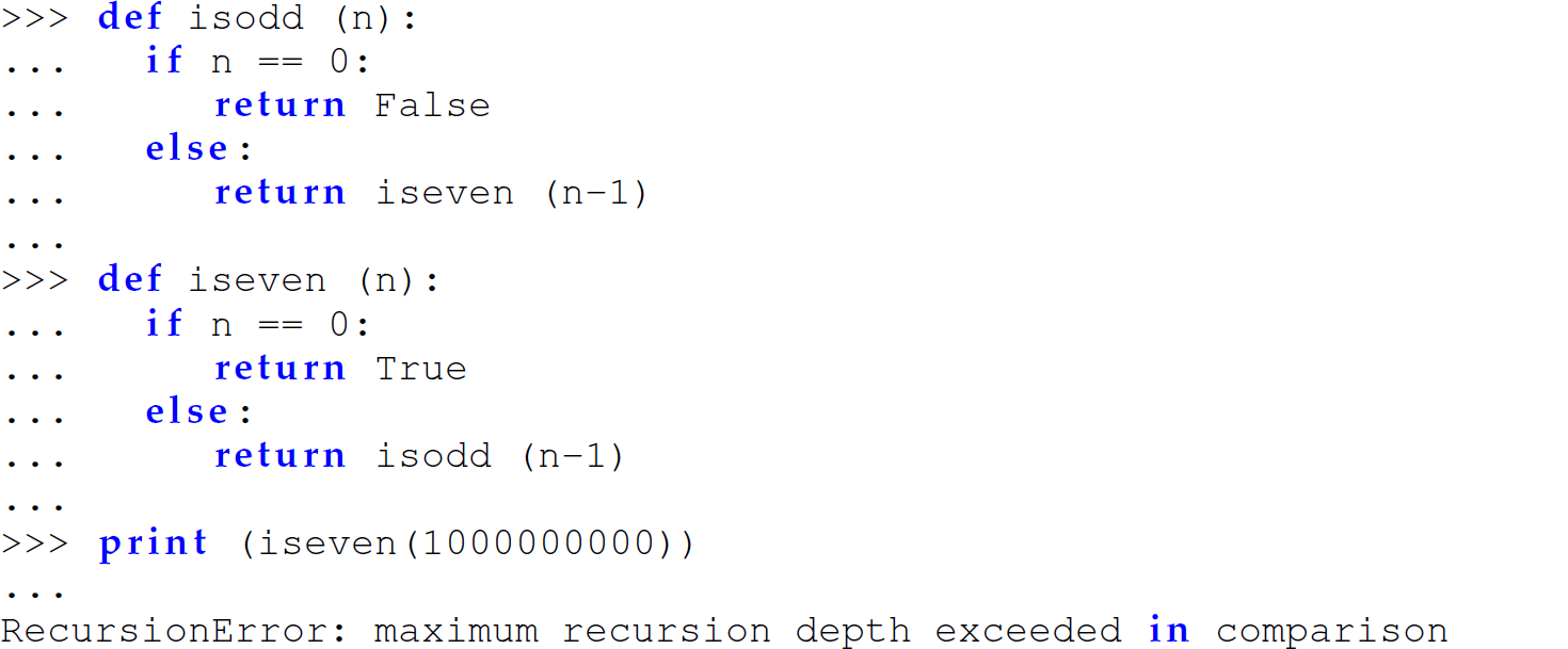
The call to isodd in the body of the definition of iseven is not tail recursion— it is simply a tail call. The same is true for the call to iseven in the body of isodd. Thus, neither of these functions is recursive independently of each other (i.e., neither function has a call to itself). They are just mutually dependent on each other or mutually recursive. Since Python does not use TCO on these non-recursive functions, this program does not run in constant memory space or without a stack.
The Scheme rendition of this Python program runs in constant space without a stack:

Thus, not only can TCO be used to optimize non-recursive functions, but it should be applied so that the programmer can use both individual non-recursive functions and recursion without paying a performance penalty.
Tail-call optimization makes functions using only tail calls iterative (in run-time behavior) and, therefore, more efficient. The revised definition of factorial using tail recursion and exhibiting iterative control behavior does not have a growing control context, so it now has the potential to be optimized to run in constant space. However, it no longer mirrors the recursive specification of the problem. By using tail recursion, we trade off function readability/writability for the possibility of space efficiency. Even so, it is possible to make recursion iterative while maintaining the correspondence of the code to the mathematical definition of the function (Section 13.8). Table 13.7 summarizes the relationship between the type of function call and the control behavior of a function.
Table 13.7 Non-tail Calls/Recursive Control Behavior Vis-à-Vis Tail Calls/Iterative Control Behavior
Functions with non-tail calls exhibit recursive control behavior: Functions with tail calls exhibit iterative control behavior: Iterative control behavior is not sufficient to eliminate the run-time stack. |
The programming technique called trampolining (i.e., converting a program to trampolined style) can be used to achieve the same effect as tail-call optimization in a language that does not implement TCO. The underlying idea is to replace a tail-recursive call to a function with a thunk to invoke that function. The thunk is then subsequently applied in a loop. Consider the following trampolined version of the previous odd/even program in Python that would not run:
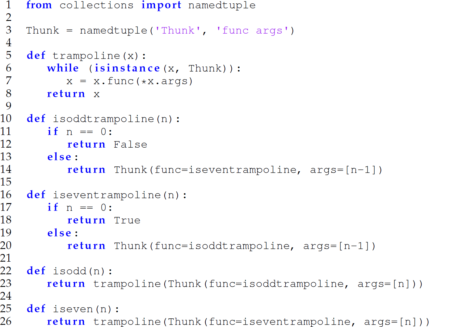
In this program, Thunk is a namedtuple, which behaves like an unnamed tuple, but with field names (line 3). We use this unnamed tuple to create the thunks that obviate the would-be recursive calls to isodd and iseven (lines 14 and 20, respectively). In lines 5–8, the function trampoline performs the computation iteratively, thereby acting as a trampoline. Therefore, we are able to write tail calls that execute without a stack:

13.7.4 Space Complexity and Lazy Evaluation
There is an interesting relationship between tail recursion and lazy evaluation in regard to the space complexity of a program. Programmers of lazy languages must have a greater awareness of the space complexity of a program. Consider the following function len defined using tail recursion in Haskell:
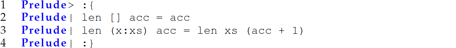
Invoking this tail-recursive definition of len in Haskell results in a stack overflow:

The following is a trace of the expansion of the calls to len:
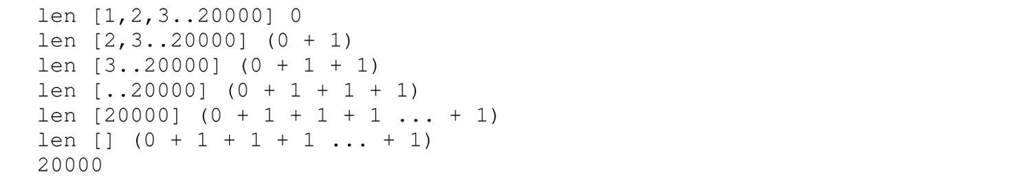
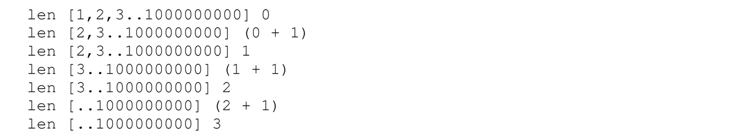
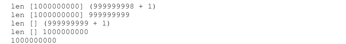
This function is tail recursive and appears to run in constant memory space—the stack never grows beyond one frame. However, the size of the second argument to len is expanding because of the lazy (as opposed to eager) evaluation strategy used. Although the interpreter no longer must save the pending computations— in this case, the additions—on the stack, the interpreter stores a new thunk for the expression (acc + 1) for every recursive call to len. Forcing the evaluation of the second parameter to len (i.e., making the second parameter to len strict) prevents the stack overflow. We can force a parameter to be strict by prefacing it with $! (as demonstrated in Section 12.5.5):

The following trace illustrates how the evaluation of the second parameter to len is forced for each recursive call:
In general, it is often recommended to make an accumulator parameter strict when defining a tail-recursive function in a lazy language.
The recursive pattern used in this definition of len is encapsulated in the higher-order folding functions. The accumulator parameter is the analog of the initial value passed to foldl or foldr. Since the combining function for len [i.e.,  ] does not use the elements in the input list, we can define len using either foldl or foldr:

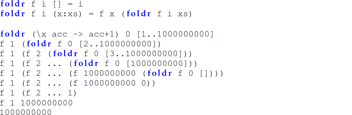
Even though this definition of len uses the accumulator approach in the combining function passed to foldr (i.e., its first parameter), its invocation results in a stack overflow:
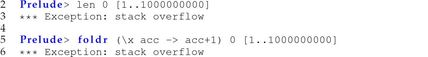
This is because foldr is not defined using tail recursion:
Conversely, foldl is defined using tail recursion:

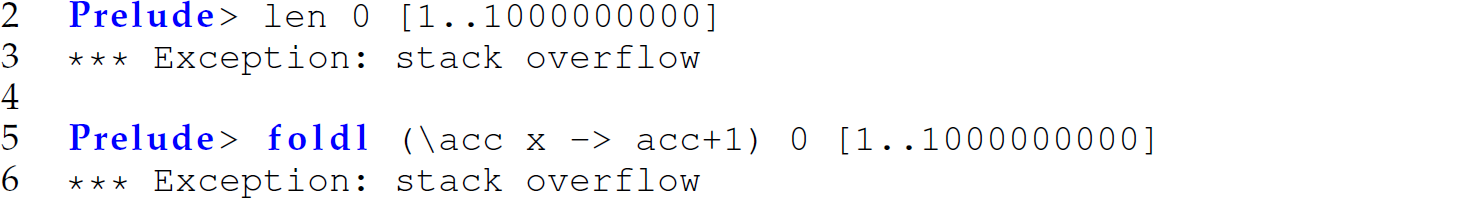
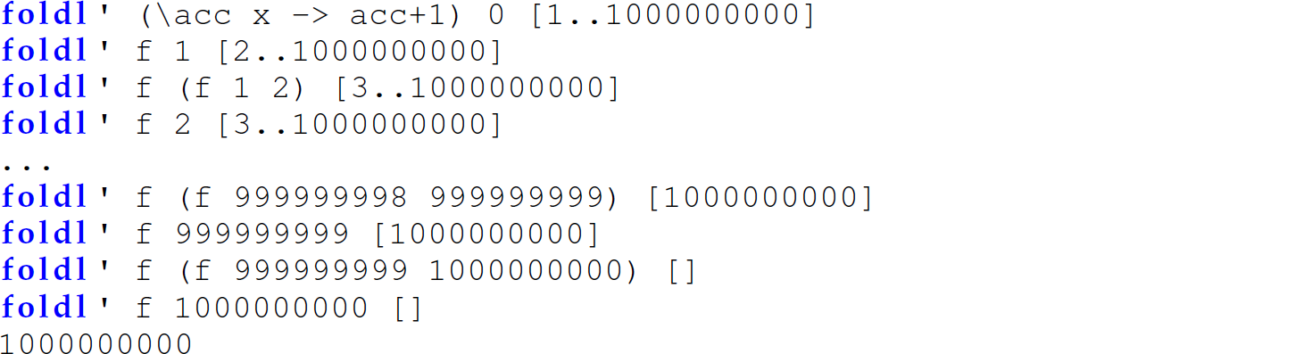
Thus, we can define a more space-efficient version of len using foldl:

Notice that in this definition of len, we must reverse the order of the parameters to the combining function (i.e., acc and x). However, this version produces a stack overflow:
The following is a trace of this invocation of len:
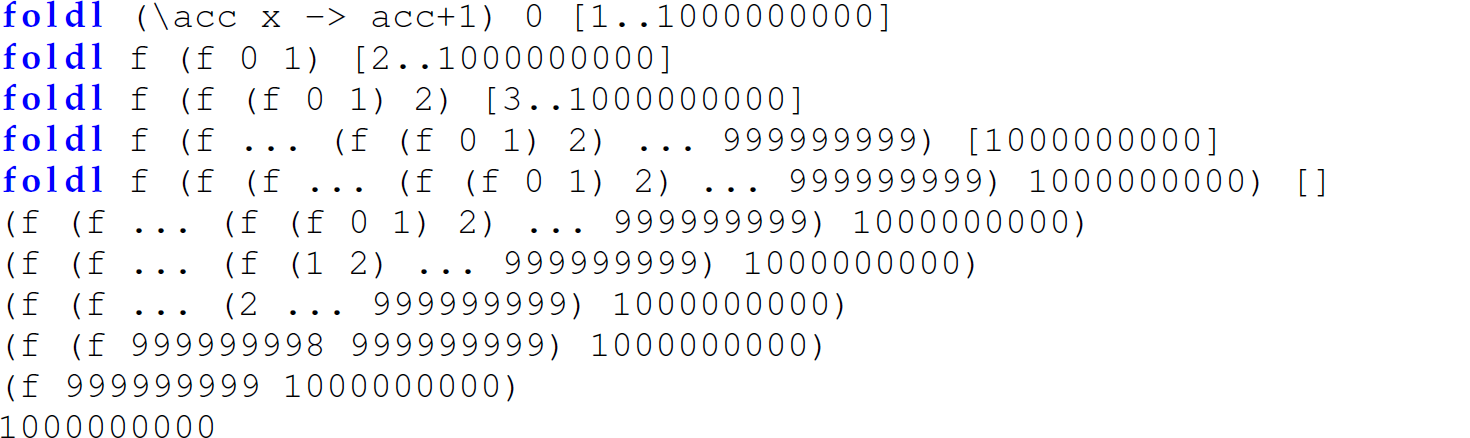
While foldl does use tail recursion, it also uses lazy evaluation. Thus, this invocation of len results in a stack overflow because a thunk is created for the second parameter to foldl—that is, the evaluation of the combining function (f i x)—for every recursive call and the second parameter continues to grow. The invocation of len builds up a lengthy chain of thunks that will eventually evaluate to the length of the list rather than maintaining a running length. Thus, this version of len behaves the same as the first version of len in this subsection.
To solve this problem, we need a version of foldl that is both tail recursive and strict in its second parameter:
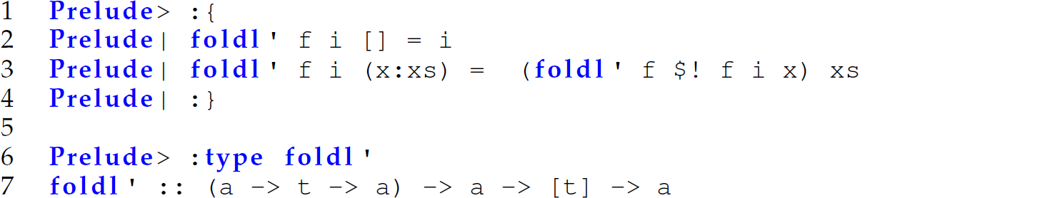
Consider the following invocation of foldl’:

The following is a trace of this invocation of foldl':
While foldr should be avoided for computing the length of a list because it is not defined using tail recursion, foldr should not be avoided in all cases. For instance, consider the following function, which determines whether all elements of a list are True:

Since (&&) is non-strict in its second parameter, use of foldr obviates further exploration of the list as soon as a False is encountered:

The following is a trace of this invocation of allTrue:

In this case, foldr does not build up the ability to perform the remaining computations. The same is not true of foldl’. For instance:

The following is a trace of this invocation of foldl’:
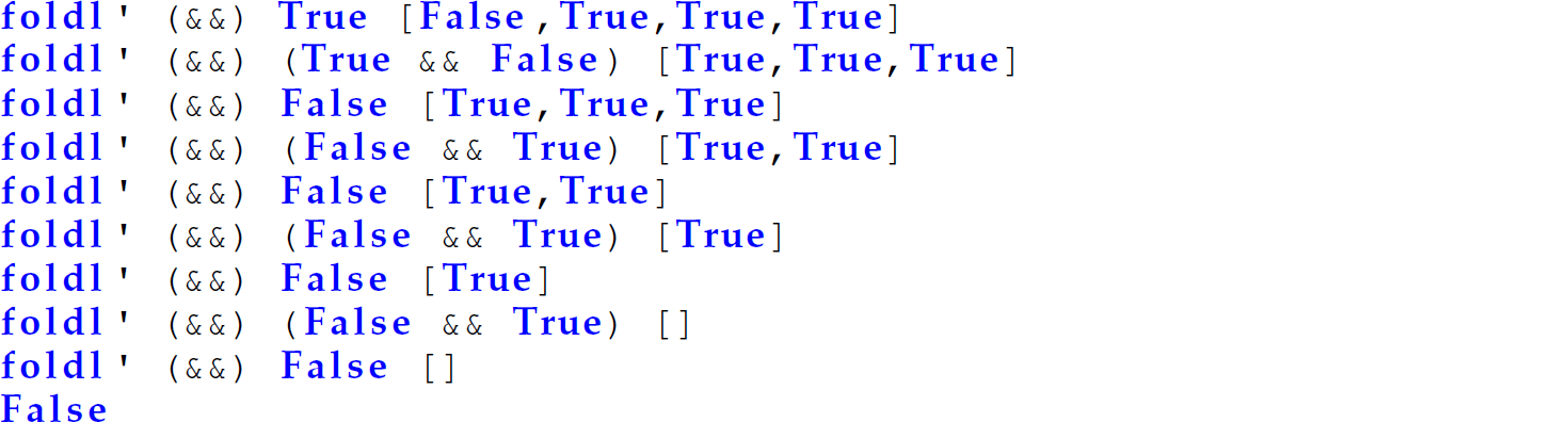
Even though this version runs in constant space because foldl’ is defined using tail recursion, it examines every element of the input list. Thus, foldr is preferred in this case. Similarly, the built-in Haskell function concat uses foldr even though foldr is not defined using tail recursion:
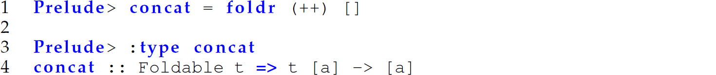
The following is an invocation of concat:

Tracing this invocation of concat reveals why foldr is used in its definition:
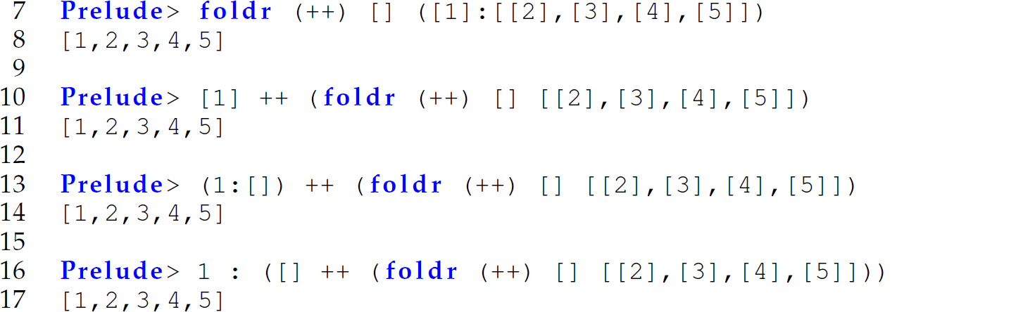
Unlike the expansion for the invocation of the definition of len using foldr in this subsection, the expression on line 16 is as far as the interpreter will evaluate the expression until the program seeks to examine an element in the tail of the result. Since we can garbage collect the first cons cell of this result before we traverse the second, concat not only runs in constant stack space, but also accommodates infinite lists. By contrast, neither foldl’ nor foldl can handle infinite lists because the left-recursion in the definition of either would lead to infinite recursion. For instance, the following invocation of foldl does not terminate (until the stack overflows):

(Note that repeat e is an infinite list, where every element is e.) However, the following invocation of foldr returns False immediately:

Since (&&) is non-strict in its second parameter, we do not have to evaluate the rest of the foldr expression to determine the result of allTrue. Similarly, since (++) is non-strict in its second parameter, we do not have to evaluate the rest of the foldr expression to determine the head of the result of concat. However, because the combining function  in len must run on every element of the list before a list length can be computed, we require the result of the entire foldr to compute a final length. Thus, in that case, foldl’ is a preferable choice.
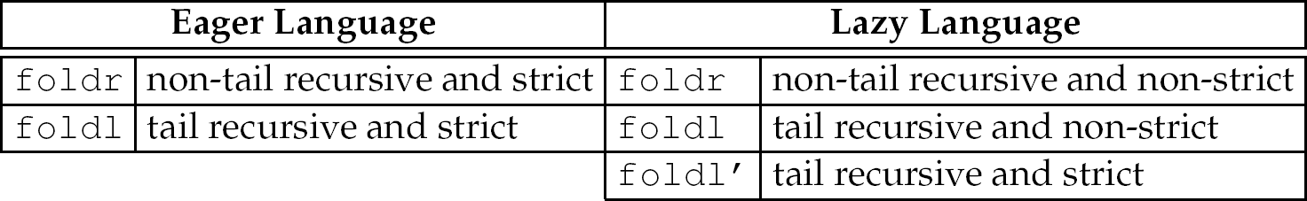
Table 13.8 summarizes these fold higher-order functions with respect to evaluation strategy in eager and lazy languages. Defining tail-recursive functions in languages with a lazy evaluation strategy requires more attention than doing so in languages with an eager evaluation strategy. Using foldl’ requires constant stack space, but necessitates a complete expansion even for combining functions that are non-strict in their second parameter. However, even though foldr is not defined using tail recursion, it can run efficiently if the combining function is non-strict in its second parameter. More generally, the space complexity of lazy programs is complex.
Table 13.8 Summary of Higher-Order fold Functions with Respect to Eager and Lazy Evaluation
We offer some general guidelines for when foldr, foldl, and foldl’ are most appropriate in designing functions (assuming the use of each function results in the same value).
Guidelines for the Use of foldr, foldl, and foldl’
In a language using eager evaluation, when both foldl and foldr produce the same result, foldl is more efficient because it uses tail recursion and, therefore, runs in constant stack space.
In a language using lazy evaluation, when both foldl’ and foldr produce the same result, examine the context:
If the combining function passed as the second argument to the higher-order folding function is strict and the input list is finite, always use foldl’ so that the function will run in constant space because foldl’ is both tail recursive and strict (unlike foldl, which is tail recursive and non-strict). Passing such a function to foldr will always require linear stack space, so it should be avoided.
If the combining function passed as the second argument to the higher-order folding function is strict and the input list is infinite, always use foldr. While the function will not run in constant space (like foldl’), it will return a result, unlike foldl’, which will run forever, albeit in constant space.
If the combining function passed as the second argument to the higher-order folding function is non-strict, always use foldr to support both the streaming of the input list, where only a part of the list must reside in memory at a time, and infinite lists. In this situation, if foldl’ is used, it will never return a result, though the function will run in constant memory space.
In general, avoid the use of the function foldl. These guidelines are presented as a decision tree in Figure 13.8.
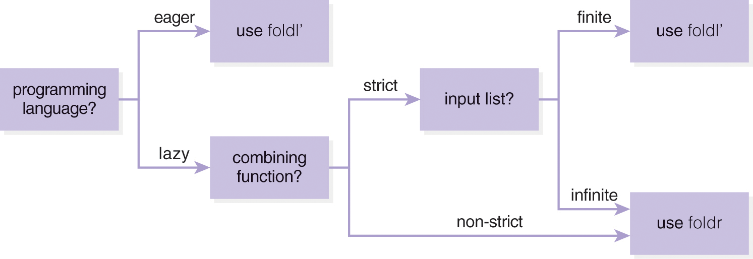
Figure 13.8 Decision tree for the use of foldr, foldl,and foldl’ in designing functions (assuming the use of each function results in the same value).
DescriptionProgramming Exercises for Section 13.7
Exercise 13.7.1 Unlike a language with an eager evaluation strategy, in a lazy language, even if the operator to be folded is associative foldl’ and foldr may not be used interchangeably depending on the context. Demonstrate this by folding the same associative operator [e.g., (++)] across the same list with the same initial value using foldl’ and foldr. Use a different associative operator than any of those already given in this section. Use program comments to clarify your demonstration. Hint: Use repeat in conjuntion with take to generate finite lists to be used as test lists in your example; use repeat to generate infinite lists to be used as test lists in your example and take to generate output from an infinite list that has been processed.
Exercise 13.7.2 Explain why map1 f = foldr ((:).f) [] in Haskell can be used as a replacement for the built-in Haskell function map, but map1 f = foldl ((:).f) [] cannot.
Exercise 13.7.3 Demonstrate how to overflow the control stack in Haskell using foldr with a function that is made strict in its second argument with $!.
Exercise 13.7.4 Define a recursive Scheme function square using tail recursion that accepts only a positive integer n and returns the square of n (i.e., n2). Your definition of square must contain only one recursive helper function bound in a letrec expression that does not require an unbounded amount of memory.
Exercise 13.7.5 Define a recursive Scheme function member-tail that accepts an atom a and a list of atoms lat and returns the integer position of a in lat (using zero-based indexing) if a is a member of lat and #f otherwise. Your definition of member-tail must use tail recursion. See examples in Programming Exercise 13.3.6.
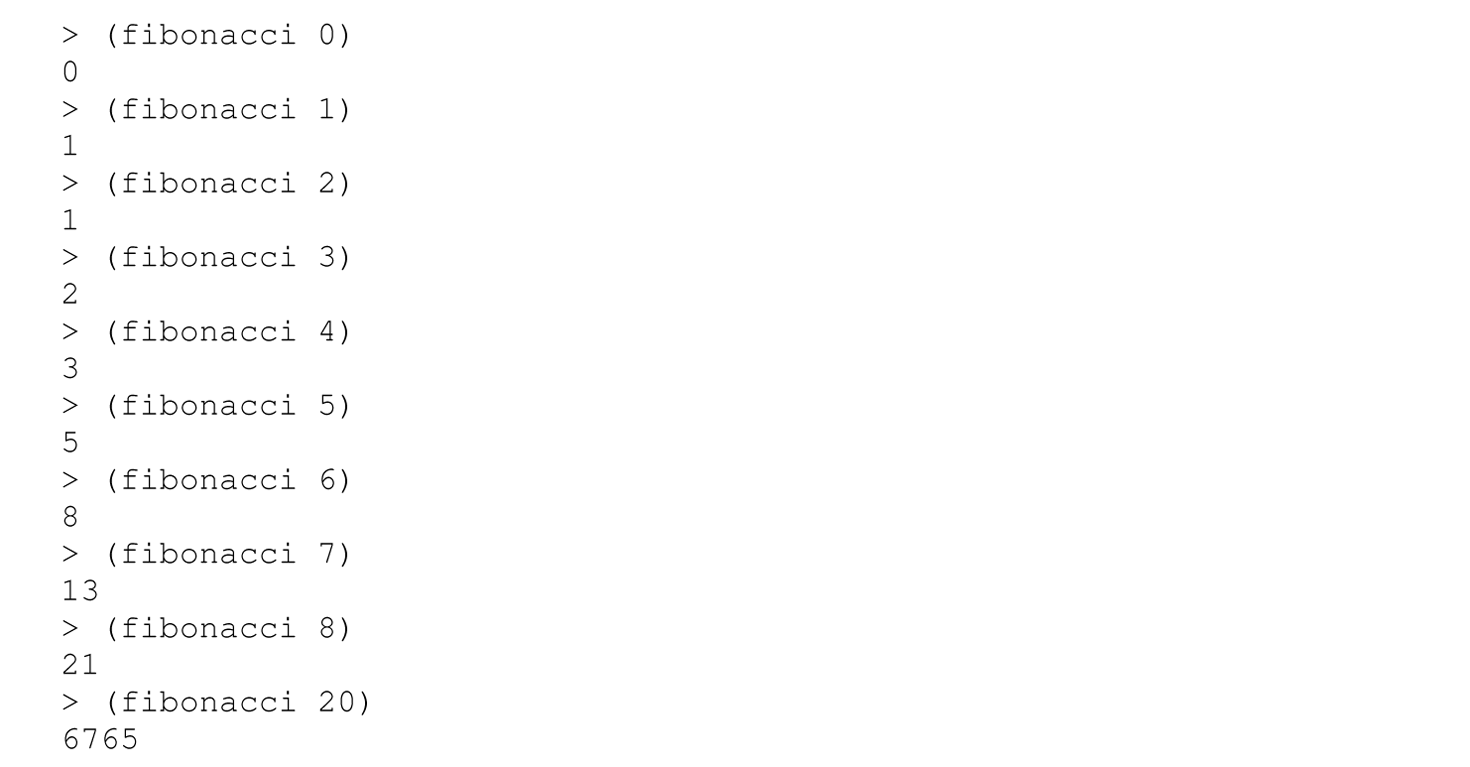
Exercise 13.7.6 The Fibonacci series 0, 1, 1, 2, 3, 5, 8, 13, 21, . . . begins with the numbers 0 and 1 and has the property that each subsequent Fibonacci number is the sum of the previous two Fibonacci numbers. The Fibonacci series occurs in nature and, in particular, describes a form of a spiral. The ratio of the successive Fibonacci numbers converges on a constant value of 1.618. . . . This number, too, repeatedly occurs in nature and has been called the golden ratio or the golden mean. Humans tend to find the golden mean aesthetically pleasing. Architects often design windows, rooms, and buildings with a golden mean length/width ratio.
Define a Scheme function fibonacci, using only one tail call, that accepts a non-negative integer n and returns the nth Fibonacci number. Your definition of fibonacci must run in O(n) and O(1) time and space, respectively. You may define one helper function, but it also must use only one tail call. Do not use more than 10 lines of code. Your function must be invocable.
Examples:
Exercise 13.7.7 Complete Programming Exercise 13.7.6 in Haskell or ML.
Exercise 13.7.8 Define a factorial function in Haskell using a higher-order function and one line of code. The factorial function accepts only a number
n and returns n!. Your function must be as efficient in space as possible.
Exercise 13.7.9 Define a function insertionsort in Haskell that accepts only a list of integers, insertion sorts that list, and returns the sorted list. Specifically, first define a function insert with fewer than five lines of code that accepts only an integer and a sorted list of integers, in that order, and inserts the first argument in its sorted position in the list in the second argument. Then define insertionsort in one line of code using this helper function and a higher-order function. Your function must be as efficient as possible in both time and space. Hint: Investigate the use of scanr to trace the progressive use of insert to sort the list.
5. This shape is comparable to the contour of an ADRS (Attack–Decay–Sustain–Release) envelope, which depicts changes in the sound of an acoustic musical instrument over time, without the decay phase: The growth of the stack is the analog of the attack phase, the base case is the analog of the sustain phase, and the computation performed as activation records pop off the stack corresponds to the release phase.
6. Tail-call optimization is also referred to as tail-call elimination. Since the caller jumps to the callee, the tail call is essentially eliminated.
7. It is tail-call optimization, not tail-recursion optimization.