
2 Norden-Rayleigh Curves for solution development
In Volume IV we discussed ways to model and estimate the time, cost or effort of recurring or repetitive tasks, but we haven’t looked at what happens before that … how long, or how much effort do we require to develop the solution that becomes the basis of our repetitive task, or of developing that one-off task, especially if it is novel or innovative?
Even if we can develop that estimate by analogy to another previous and not too dissimilar task, or by parametric means, there is nothing obvious so far that helps us say how that estimate might be profiled in time; a problem that is often more of a challenge perhaps than getting the base value itself.
Perhaps the best-known model for doing this is the Norden-Rayleigh Curve, but there are others that we might refer to collectively as ‘Solution Development Curves’.
2.1 Norden-Rayleigh Curves: Who, what, where, when and why?
John William Strut, the 3rd Lord Rayleigh, was an English physicist who discovered the gas Argon (for which he won a Nobel Prize in 1904); he also described why the sky appears to be blue. (We could say that he was one of life’s true ‘Blue Sky Thinkers’ who knew how to strut his stuff.) More importantly for us as estimators, he came up with the Probability Distribution that bears his title, not his name. (The Rayleigh Distribution has a better ring to it than the Strut Distribution, doesn’t it? That would make it sound rather like a component stress calculation.) The Rayleigh
A word (or two) from the wise?
'If we knew what it was we were doing, it would not be called research, would it?'
Attributed to Albert Einstein
Physicist
1879-1955
Distribution is often used to model reliability and failure rates, but has numerous other applications as well.
In 1963, Peter Norden contemplated the life cycle of a basic development process from a pragmatic rather than a purely theoretical perspective in relation to the software engineering sector. Paraphrasing his deliberations, which we might summarise as ‘trial and error’, the process of natural development is:
- Someone makes a request for something that doesn’t exist
- Someone comes up with a bright idea for a solution
- Resource is deployed to scope the requirements in more detail and identify what they mean, and in so doing creates a list of problems to overcome (beginning to sound familiar?)
- More resource is deployed to overcome the problems
- These problems are overcome but throw up more understanding of the needs of the solution but also raises other problems, and perhaps better ways of tackling what has already been done … all of which need more resources. (If this sounds like we don’t know what we’re doing, then just reflect on the thoughts of Albert Einstein (attributed by Amneus & Hawken, 1999, p.272).)
- Eventually the combined resources break the back of the mound of problems, and less and less new challenges are discovered, and existing solutions can be used to complete the remaining tasks, which ultimately need fewer resources
- Eventually, the solution is developed (although often the engineers will probably have thought of some enhancements and have to be forcibly prised away from the project (a crowbar is a useful project management tool in this instance!)
By analysing the profile of many such development curves, Norden concluded that a truncated Rayleigh Distribution was a good fit. The Rayleigh Distribution appeared to perform well as a model for the ramp-up of resources to a peak before tapering off again over time. The only problem is that a Rayleigh Probability Distribution extends to positive infinity, and so from a pragmatic point of view, it has to be truncated. By convention (implying that this is accepted practice, rather than something that is absolutely correct), this is taken to be at the 97% Confidence Level of a Rayleigh Distribution (Lee, 2002). However, this does cause some issues, as we will explore later, and there may be some practical alternatives we can consider instead. In other words, there is no compelling reason why we cannot have more than one convention, just as we have with physical measurement scales (Imperial vs. Metric).
Although its roots lie in the project management of software engineering projects, further studies by David Lee and others (e.g. Gallagher & Lee, 1996) have shown that the basic principles of the Norden-Rayleigh Curve can be extended to more general research and development tasks. In particular, it has been shown to fit some major defense development programmes (Lee, Hogue & Hoffman, 1993). This seems to indicate that there is an underlying consistency and commonality across complex engineering development processes. This latter article demonstrated that the cost and schedule of such development programmes could be normalised in terms of their relative scales into a single curve – the Norden-Rayleigh Curve. The implication for us, therefore, is that (theoretically speaking) we can stretch or compress the overall curve without losing its basic shape or integrity. It implies also that there are two scale factors, one for each of the horizontal and vertical scales. However, from a more empirical perspective, this does not necessarily work once we have commenced the development process.
2.1.1 Probability Density Function and Cumulative Distribution Function
Although the Norden-Rayleigh Curve is based on the Rayleigh Distribution, the Probability Density Function and Cumulative Distribution Function are not the most elegant to read or follow.
The good news is that the Rayleigh Distribution is actually a special case of the Weibull Distribution in which the Weibull parameters α = 2 (always) and β = l√2, where l is the Rayleigh Distribution Mode parameter. Why is this good news? As we discussed in Volume II Chapter 4 on Probability Distributions (unless you skipped that particular delight and left me talking to myself) Microsoft Excel has a special in-built function for the Weibull Distribution:
WEIBULL.DIST(x, alpha, beta, cumulative)
To calculate either the probability density value for x (cumulative = FALSE), or the Cumulative Probability (cumulative = TRUE) with Shape Parameter, alpha and Scale Parameter beta
In earlier versions of Microsoft Excel, the function was simply:
WEIBULL(x, alpha, beta, cumulative)


So, a Rayleigh Distribution would be WEIBULL.DIST(x, 2, Mode √2, TRUE or FALSE) in Microsoft Excel depending on whether we want the CDF or PDF values.
To convert this into a Norden-Rayleigh Curve to represent a time-phased profile of the development cost, we simply express the independent variable, x to be time from the project start, multiplied by the estimate of the total cost … and then decide where we are going to truncate it.
2.1.2 Truncation options
As the distribution is scalable in the sense that we can stretch or compress it vertically to change the project outturn values, or we can stretch or compress it horizontally to reflect a change in the chosen rate of development, i.e. its schedule, then we only need to examine the relative properties against a ‘standard distribution’. For this purpose, we will only consider the cost profile values (vertical axis) in relation to the percentage of the final outturn cost being 100%. For the horizontal axis, we will look at time elapsed from the start relative to a multiplier of the mode position. For simplification, we will define the mode to occur at time 1 relative to a start time of 0. Table 2.1 and Figure 2.3 illustrates the invariable percentage values from the Cumulative Distribution Function.
As we will observe, the Mode occurs when Development is theoretically 39.347% complete (that’ll be at around 40% in Estimating Speak!).
The ‘conventional’ truncation point for a Norden-Rayleigh Curve is at the 97% Confidence Level (Lee, 2002), which always occurs at 2.65 times the Mode. (We might as well call it two and two-thirds.)
However, for those of us who are uncomfortable with this, being perhaps a somewhat premature truncation point, we will see that there are other Rules of Thumb we can use that infer a truncation at different levels of decimal place precision closer to 100%, such as 3.5 times the Mode. The nice thing about the 3.5 factor is that it is visually close enough to 100% (see Figure 2.1) and it is also analogous to the Normal Distribution’s ‘standard Confidence Interval’ of the Mean +3 Standard Deviations (99.73%).

Table 2.1 Cumulative Distribution Function of a Standard Rayleigh Probability Distribution

Figure 2.1 Norden-Rayleigh Curve Compared with a Standard Rayleigh Probability Distribution
The question we should be asking ourselves when we select a truncation point is:
How precisely inaccurate do we want our profile to be?
Some of us may be wondering why we have highlighted the 63.212% at the Mode x SQRT(2) in Table 2.1. This links back to the standard property of a Weibull Distribution (Volume II Chapter 4 if you missed that particular delight).
There are three benefits to be had with choosing an end-point at the 3.5 factor point in time:
- We don’t ‘have to’ factor the vertical scale to accommodate the truncation because if we do choose to do so, the Uplift Factor is only 1.0022. (Our development estimate is not going to be that precise, is it?)
- The PDF can be used to model the resource profile by time period without a sudden cut-off implied by the conventional approach (see Figure 2.1.) However, if this is what happens in reality, then perhaps we should adopt the convention of a 2.65 Truncation Ratio unswervingly at the 97% Completion Level.
- We don’t have a long and procrastinated tail to higher levels of hypothetical precision for true values greater than 3.5 times the Mode.
There is a case to be made that a value of 3 is an acceptable compromise, achieving a level of some 98.9% with a much easier multiplier to remember and without the additional crawl through to 3.5 for a paltry 0.9%. (Try using that argument with an accountant when the total is in the millions or billions!)
Any truncation activity should consider what is likely to happen in the environment in question. Ask ourselves whether any development is truly completed in an absolute sense. If the answer is ‘yes’ then in terms of recurring production learning there would be no contribution required from engineering etc. So at what point do we just say ‘enough is enough’ and terminate the development (probably to the annoyance or relief of some engineers)?
2.1.3 How does a Norden-Rayleigh Curve differ from the Rayleigh Distribution?
The main difference between the two is one of scale. The cumulative of any probability distribution is always 100% (or 1) whereas the Norden-Rayleigh Curve is geared to the final outturn cost. This is complicated because the Rayleigh Distribution as a special case of a Weibull Distribution ‘goes on indefinitely’ and by implication only reaches 100% at infinity. Design and Development programmes do not go on indefinitely (although sometimes, to some of us, some of them appear to go on forever) and a practical limitation has to be placed on them, hence the manual truncation of the cost-schedule curve.
For the Formula-philes: Norden-Rayleigh Curve
Consider a Norden-Rayleigh Curve with an outturn value of CT (the vertical scale parameter) and a completion time of T relative to its start time at zero, and a mode at time λ (the horizontal scale parameter) Let C∞ be the notional cost at infinity if development was allowed to continue indefinitely.

In Figure 2.2, we can see the characteristic asymmetric S-Curve of a Cumulative Rayleigh Distribution Function (CDF) with its positive skew. In comparison, we can see how the Norden-Rayleigh Curve truncates and uplifts the Rayleigh Distribution. In this example we have truncated and uplifted the Rayleigh Distribution at the 97% Confidence/Completion Level.
Note that we have not stipulated any definition with regards to the scale of the Time axis. That’s because we can define it in relation to any scale, be it days, weeks, lunar months, calendar months or years; it can also be in hours, minutes, seconds, decades, centuries etc. but these are totally impractical which is why I never mentioned them … oh! I just have now … well please ignore them.

Figure 2.2 Norden-Rayleigh Curve as a Truncated Cumulative Rayleigh Probability Distribution
For the Formula-philes: Time is a relative term with a Norden-Rayleigh Curve
Consider a Norden-Rayleigh Curve with an outturn value of CT (the vertical scale parameter) and a completion time of T relative to a start time of zero, and a mode at time λ.
Let the Cumulative Cost at time t on a Norden-Rayleigh Curve with


We can easily redefine the Time axis measurement scale by applying different scale factors. For instance, the scale factor to convert a NRC expressed in years to one expressed in months is 12. Table 2.2 illustrates that there is no difference. Both curves use the same Excel function for the Rayleigh Distribution but use the different Time scales.
The left hand Curve uses WEIBULL.DIST(year, 2, 1.414, TRUE) where 1.414 is the Mode of 1 multiplied by the Square Root of 2.
The right hand Curve uses WEIBULL.DIST(month, 2, 16.971, TRUE) where 16.971 is the Mode of 12 multiplied by the Square Root of 2
The Norden-Rayleigh Curve equivalent of the Rayleigh Probability Density Function (PDF) is the relative resource loading or cost expenditure ‘burn rate’ at a point in time. We can see the consequences of the truncation and uplift of the former to the latter in Figure 2.3.

Table 2.2 Norden-Rayleigh Curves are Independent of the Time Scale

Figure 2.3 Implication of a Norden-Rayleigh Curve as a Truncated Rayleigh Probability Density Function
2.1.4 Some practical limitations of the Norden-Rayleigh Curve
Dukovich et al (1999) conducted an extensive study into the practical application of Norden-Rayleigh Curves and expanded our understanding of how, when and why they are appropriate in the research and development environment:
- The characteristic shape and constancy of the Rayleigh Distribution implies that there is a relationship between the resource loading and the total effort or cost expended in achieving the development goals.
- Any development project has a finite number of problems which must be overcome but not all these problems are known at the start of the project.
- Most of the development cost incurred must be the labour cost incurred by the development team in the time they take to resolve problems. Non-labour costs should be relatively small. (It is probably safe for us to assume in many instances that any costs for outsourced development is considered to be predominantly labour costs.)
- The total number of people actively engaged on the development at a given time is in directly proportion to the number of problems being worked at that time, and their relative complexity (Norden, 1963).
- In resolving problems, this uncovers other problems which were previously unforeseen. This effectively limits the introduction of new members of the team (and their skill requirements) until the problems are identified. As a consequence, it is often impractical to compress development timescales except in cases where ‘resource starvation’ is a matter of policy, e.g. where it is temporarily unavailable due to other priorities. If additional resource (people) are added prematurely, this adds cost but achieves virtually nothing as there is a risk that they will be under utilised.
A word (or two) from the wise?
Augustine's Law of Economic Unipolarity:
'The only thing more costly than stretching the schedule of an established project is accelerating it, which is itself the most costly action known to man.'
Norman R Augustine
Law No XXIV
1997
As Augustine (1997, p.158) rightly points out, tinkering with a schedule once it has been established is going to be expensive.
Dukovich et al (1999) concurred with Putnam & Myers (1992) that the development project must also be a bounded development project through to its completion with a consistent set of objectives, i.e. no change in direction. However, they did consider the aspect of concurrent or phased development projects and we will return to this later in Section 2.2.1.
In essence, the development objective is expected to remain largely (if not totally) unchanged, and there is no realistic expectation that spend profiles on incremental development projects, or ones whose objectives evolve over time will be adequately represented by a Norden-Rayleigh Curve. Likewise, any project that we undertake that has a finite resource cap which is less than that required to meet the emerging problems to be solved, may not follow the pattern of the Norden-Rayleigh Curve. However, again we will revisit that particular scenario later.
In some respects, it may seem to be very limiting and that a Norden-Rayleigh Curve might only be applicable to small, relatively simple, research and development projects. Not so! Using data published by the RAND Corporation (Younossi et al, 2005), we can demonstrate that they work for major Aircraft Engineering & Manufacturing Development (EMD) programmes such as the United States F/A-18 and F/A-22 Fighter Aircraft (except they would have spelt it with one ‘m’ not two).

Figure 2.4 Indicative Example of F/A-18 EMD Costs Plotted Against a Rayleigh Distribution
Source: © 2005 RAND Corporation
Younossi O, Stem DE, Lorell MA & Lussier FM, (2005) Lessons Learned from the F/A-22 and F/A-18 E/F Development Programs, Santa Monica, CA, RAND Corporation.
In fact, the normalised expenditure profile is a reasonable approximation to a Rayleigh Distribution for F/A-18E/F, heralded as a successful development programme in terms of cost and schedule adherence (Younossi et al, 2005), as we can see from Figure 2.4. The Actual Cost of Work Performed data (ACWP) has been extracted with permission from Figure 4.3 of the RAND Report (Younossi et al, 2005, p.51) and superimposed on a Norden-Rayleigh Curve; the tail-end is less well-matched but it does recover in the latter stages. We might speculate that this could be as a consequence of funding constraints in the latter stages.
In respect of the F/A-22 as shown in Figure 2.5, the ACWP data (extracted from Younossi et al (2005) Figure 4.1, p.39) is a very good fit to the Norden-Rayleigh Curve … at least as far as the data published allows us; we will note that it is incomplete with potentially an additional 7% cost to be incurred to complete the development programme. It is possible that this spend profile was subsequently truncated. We will revisit the implications of this discussion in Section 2.5.
We might want to reflect on this. Military Aircraft Development Projects are rarely ‘single, integrated development projects’ with unchanging objectives as allegedly required for a Norden-Rayleigh to be valid, but they seem to work well here … and potentially without the need for the ‘conventional’ truncation at 97%. Here we have used the 3.5 Truncation Ratio at the 99.97% Confidence Level.
Putnam and Myers (1992) had previously applied a variation of the Norden-Rayleigh Curve to the development of software applications. These are often referred to as the Putnam-Norden-Rayleigh Curve (or PNR Curves) and date back to 1976.

Figure 2.5 Indicative Example of F/A-22 EMD Costs Plotted Against a Rayleigh Distribution
Source: © 2005 RAND Corporation
Younossi O, Stem DE, Lorell MA & Lussier FM, (2005) Lessons Learned from the F/A-22 and F/A-18 E/F Development Programs, Santa Monica, CA, RAND Corporation.
However, there are many instances (Dukovich et al, 1999) where the principles of a Norden-Rayleigh Curve are not met and hence the Rayleigh Distribution is not (or may not) be appropriate:
- a) Software Development projects characterised by:
- A phased development and release of interim issues
- Evolving or changing development objectives following each interim release
- An emphasis on ‘bug fixing’ and minor enhancements to existing versions (Yes, yes, I can hear the cynics muttering ‘Well, that’ll be all software projects then!’)
- b) Phased Development projects/contracts in which:
- The objectives of each development phase are not clearly distinct from each other
- There is a gap between the phases, and the resourcing strategy differs for each phase
Note: where the resourcing strategy is the same, the gap may be accommodated by ‘stopping the clock’ for the duration of the gap, or slowing it down during the ramp down of one phase and the ramp-up of the next. We will look at this more closely in Section 2.2.4.
- c) Independent Third-Party Dependencies (sounds like an oxymoron but isn’t) in which:
- The development requires an activity to be performed that is not in the control of the development project but is essential to the natural ongoing development process. This could include Government Testing using dedicated facilities for which there are other independent demands and constraints on its availability
- There is another parallel development programme (with its own objectives) on which there is an expectation of a satisfactory outcome to be exploited by the current project
- The delays caused by independent third-parties lead to additional resource ramp-downs, the inevitable attrition of key members of the team and subsequent ramp-up again after the delay … possibly with new team members
Note: It may be possible to accommodate such delays by ‘stopping the clock’ or slowing it down for the duration of the delay if this occurs during the ramp-up or ramp-down phases of the project rather than during the main problem resolution phase. Again, we will look at this more closely in Section 2.2.4.
- d) Multiple Prototype Development Programmes in which:
- Each prototype is a variation of the first and there is a high degree of commonality requiring the purchase of many common items
- There are multiple hardware purchases, requiring little or no development investment, but which are disproportionate to the scale of the development tasks interspersed between the purchase required
- The procurement activity and delivery is often phased to attract economically favourable terms and conditions from suppliers, creating spikes and plateaus in expenditure profiles
- The unique development task peculiar to each new prototype variant may be shown to follow the pattern of a Norden-Rayleigh Curve if resource, time and cost are recorded separately for each prototype, but where the same resource is working on multiple tasks this may ‘distort’ the profile of every prototype
In all cases, especially where the development extends across a number of years it is strongly recommended that all costs and labour time are normalised to take account of economic differences such as escalation, and any adjustments to accounting conventions including changes in overhead allocations (see Volume I Chapter 6).
2.2 Breaking the Norden-Rayleigh ‘Rules’
Despite the tongue-in-cheek nature of the ‘Law of Economic Unipolarity’ (Augustine, 1997) to which we referred in Section 2.1.2, stretching the schedule of development programmes is not unknown and as Augustine’s 24th Law suggests is not without its consequences. However, let’s look at schedule elongation due to four different reasons:
- Additional work scope (on top of and not instead of the original objectives)
- Correction of an overly optimistic view of the problem complexity
- Inability to recruit resource to the project in a timely fashion
- Premature resource reduction (e.g. due to budget constraint)
2.2.1 Additional objectives: Phased development (or the ‘camelling’)
In theory, this could be the easiest to deal with. It is not unreasonable to assume that the additional development objectives also follow the Norden-Rayleigh Curve and principles. If the additional work scope is independent of the original work scope other than it may be dependent of the satisfactory resolution of some problem from the original scope in order to begin or progress beyond a certain point. Let’s consider the first of these semi-independent conditions.
Suppose we have an additional 20% work scope that we can start when the original project is around two-thirds complete; that would be at Time period 1.5 relative to a mode at time period 1. Figure 2.6 shows the addition of two Norden-Rayleigh Curves with identical relative modes that only differ in their start date and their modal value. The resultant curve, although positively skewed, is not a Norden-Rayleigh Curve as the ratio of the duration to the Mode is 5.

Figure 2.6 Phased Semi-Independent Developments with an Elongated Single Hump

Figure 2.7 Phased Semi-Independent Developments with Suppressed Double Hump
This is something of a fluke because if the start point of the second development was earlier or later, or its duration was shorter, we would most probably get a suppressed double hump as shown in Figure 2.7. So, if the first example was a Dromedary (single hump) Camel, then this is tending towards being more of a Bactrian (double-humped) Camel. The later into the original schedule the additional work is commenced, and the more significant the work content is, then the more Bactrian-like the development resource profile will look.
However, if the additional work scope is more interdependent on the original objectives, then it may be more appropriate to consider this to be more akin to an underestimation of the project complexity …
2.2.2 Correcting an overly optimistic view of the problem complexity: The Square Rule
In this situation, we are considering the situation where perhaps the original estimate or the allocated budget was too low (Shock, horror! It’s true: estimators do get it wrong sometimes, and other times they just get overruled!)

Figure 2.8 The Penalty for Underestimating the Complexity of Solution Development
If the project is being allowed to ramp-up resource naturally as new problems are discovered then the principles will continue to apply, reaching a higher mode at a later time, and eventually finishing later than originally planned. In cases like this, we can use the inviolable shape property of the Norden-Rayleigh Curve to assess the likely cost of schedule slippage. In fact, it’s a Square Rule; a percentage increase in schedule generates an increase in cost equal to the square of the slippage increase, adding some insight into Augustine’s observation that schedule slippage is extremely expensive.
We can illustrate this with Figure 2.8. The NRC Cost Density Functions in the left-hand graph show that the actual mode occurred 50% later than the budgeting assumption with a corresponding knock-on to the project completion date. Also, we have the situation where the actual Modal Value was 50% greater than that assumed in the budget, but that initially the ramp-up rates were the same. In the right-hand graph, we show the corresponding cumulative cost distributions; whilst the development project ‘only’ took 50% longer than planned, the outturn cost was a whacking 125% over budget, i.e. 225% is the square of 150%. Such is the potential penalty for underestimating engineering complexity, giving us our Square Rule.
This rule also works in cases where the development turns out to be less complex than originally expected and we find that we don’t need to ramp-up our resource as high and for as long. In theory, this allows us to shorten the schedule with the consequential square root benefit on cost.
However, do not confuse natural early completion with artificial compression …
The same principle of squaring the scale factors can be extended to any distribution-based resource profile and its associated Cumulative S-Curve, as illustrated by the Formula-phobe call-out on the cost of schedule slippage based on a Triangular Distribution.
Shortening a project schedule because the project is simpler than expected is not the same as compressing the schedule artificially to accelerate the completion date without any corresponding reduction in assumed complexity. The intellectual thought processes and physical validation results synonymous with Solution Development generally cannot be hastened.
For the Formula-phobes: Square Rule for the cost of schedule slippage
If we accept the principles and properties of the Norden-Rayleigh Curve then the effective end date is some 3.5 times the Mode or point of peak resource or expenditure.
The S-Curve is the area under the resource profile graph. So if the resource is proportionately taller and lasts for longer, then the area will increase by the product of the two. If the two proportions are the same then the profile will be increased by the square of the slippage.
Consider a Triangular Distribution as an analogy. (We could liken the Norden-Rayleigh Distribution to be a sort of ‘rounded triangle’.)
As we may recall from school Maths lessons (unless those memories are still too painful), the area of a triangle is always: ‘Half the Base times the Perpendicular Height’

If we scale both the height and the base by the same factor we keep the same shape but change the area by the square of the scaling factor. In the example, we have scaled the base and height by 1.5 and the area is then 2.25 times bigger. The smaller triangle has an area of 4, whilst the area of the larger dotted triangle with the same basic shape, has an area of 9. Each mini triangle has an area of 1.
For the Formula-philes: Norden-Rayleigh Square Rule
Consider a Norden-Rayleigh Curve (NRC) with an Outturn Cost of Cλ and a Mode at λ, based on a truncated Rayleigh Distribution using an uplift factor of k:

2.2.3 Schedule slippage due to resource ramp-up delays: The Pro Rata Product Rule
If we accept the principles and properties of the Norden-Rayleigh Curve, then the number of problems to be solved are finite, and many of these problems are unknown until earlier problems are investigated (problems create problems.) If we cannot resource our project quickly enough, we may discover a new problem that has to wait until the resource is available. Let’s say that we eventually resource up to the same level of resource as planned, albeit late. We can exploit the shape integrity of the Norden-Rayleigh Curve to estimate the impact of the schedule delay. In this case the cost increase is pro rata to the schedule slippage as illustrated in Figure 2.9. Here, the actual Mode occurs 50% later than expected and the overall project also finishes 50% later. In contrast to the previous scenario, we are assuming that the peak resource (Modal Value) remains the same; the net result is that the cost overrun is pro rata to the schedule slippage, giving us a Pro Rata Product Rule.
Now you might well ask why we have referred to this as ‘Pro Rata Product Rule’ and not simply the ‘Pro Rata Rule’. Well, consider this … in some instances we may not need to resource up to the same level as existing resource may be freed up to look at new problems, thus reducing the need for additional resource. In this case, we may find that there is no impact on cost outturn even though there is a schedule slippage. Let’s look at that one in Figure 2.10. In this case even though the schedule slips by 50%, the actual peak resource is only two-thirds of the budgeted level. If we take the product of the Peak Resource factor (i.e. ⅔) and the Schedule Change factor (1.5), we get unity, i.e. our factors cancel out.
I can see that one or two of us have spotted that the previous Square Rule is just a special case of the Pro Rata Product Rule, in which both factors are the same. Maybe we can exploit this in the third and most difficult context, i.e. when budget restrictions are introduced after the project has commenced.

Figure 2.9 The Penalty of Late Resourcing

Figure 2.10 The Opportunity of Late Resourcing
2.2.4 Schedule slippage due to premature resource reduction
Here we are considering a development project in which the project has already been started and has been geared to an original schedule, but later, possibly after the peak resource has been passed, funding is restricted going forward, or resource is re-prioritised to another project. In this case, stretching the cycle due to a budgetary constraint disrupts Norden’s hypothesis of how and why resource ramps up sharply initially as new problems are discovered, and then decays later over a longer period.
It can be argued that the need to take off resource quickly or prematurely leaves some problems unresolved until the remaining resource is free to take them on board. Potentially this could imply some duplication of prior effort as they review the work done previously by those who have now departed the project (or worse, they simply just repeat it). How do we deal with such an eventuality, or do we just throw our hands in the air and resign ourselves to the fact that they will probably just blame any overspend on the estimator? (We can probably still feel the pain and indignity of it.)
Let’s consider a controlled slow down, where for reasons of cash flow, or alternative business priorities, the development project needs to free up half its resource from a point in time. Inevitably, the schedule will slip, but what will happen to the cost? Let’s look at how we might tackle it from a few different perspectives:
- Slowing Down Time (The Optimistic Perspective)
- Marching Army Penalty (A More Pragmatic Perspective)
- Creating a Bactrian Camel Effect (The Disaggregated Perspective)
- Modal Re-positioning (A Misguided Perspective)
Let’s look at each in turn.
(1) Slowing Down Time (The Optimistic Perspective)
We could say that anyone who thinks that they can slow down time is optimistic (or deluded!).
From an optimistic perspective, we could argue that had we known that we would only have access to half the resource in the first place, then we might have assumed that the development cycle would have taken twice as long. We could splice two Norden-Rayleigh Curves together using the fully resourced curve until the resource capping is imposed, followed by the capped resourced curve until the development is completed. In effect this is the same as saying that from the point of the resource reduction to 50% of the previous level, we can achieve the same resolution to our challenges but in twice the time.
The easiest way to create the data table for this is to slow down time! The following procedure explains what we mean by this.
- Create the normal Norden-Rayleigh Curve for both the Cost Density Function and the Cumulative Distribution Function (as per the Budget) based on a truncated Rayleigh Distribution.
- Multiply the Cost Density Function by the resource reduction factor (in this example 50%).
- Create a second Time variable which matches the original time used in Step 2 UNTIL the point at which the artificial spend constraint is to be imposed. After that point increase the time increment by dividing by the resource reduction factor. This in effect slows down time!
See the example in Table 2.3 (showing values until time = 2 for brevity) and Figure 2.11. The left hand graph depicts the resource profile and the right hand graph the cumulative cost profile.
Now we can see why this approach is an optimistic one (some would say ‘naïve’) in that there is no prime cost penalty, only a schedule penalty, irrespective of when the
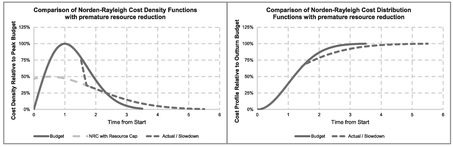
Figure 2.11 Optimistic View of Premature Resource Reduction

Table 2.3 Stretching Time to Model the Optimistic View of Premature Resource Reduction
intervention occurs! (Any cost penalty will come from additional inflationary aspects due to slippage in time.) The schedule penalty is to double the time remaining to completion.
For many of us, however, that will seem to be counter-intuitive, and certainly conflicts with the observations of Augustine in relation to schedule slippage. The reason that it has happened is that it makes the presumption that there is no handover or rework penalty. It implies that had we started earlier with half the resource then we would have reached the same point in development at the same time. (Really? I wish you luck with that one!)
Let’s look at the basic principle of it from a more pessimistic viewpoint with a handover or rework penalty.
(2) Marching Army Penalty (A More Pragmatic Perspective)
In terms of a penalty (conspicuous by its absence in the previous option) one possible model we might consider adopts the principle of the ‘Marching Army’ (some people prefer the term ‘Standing Army’):
- We follow a standard Norden-Rayleigh Curve until the intervention point (in this case at period 1.5).
- We reduce the level of resource available to us … in this example to a half.
- We create another Norden-Rayleigh Curve using the reduced resource and a proportionately longer schedule (in this case double the schedule with half the resource) and align it horizontally so that it intersects the original curve at the position equivalent to the reduced resource level.
- We maintain a Marching Army of constant resource from the point at which we reduced the resource at step 2 until the slow-down curve from step 3 intersects the original curve from step 1 (as determined in step 3).
- We then follow the slow-down curve through to completion, gradually reducing the resource.
- The cumulative version is then the two Norden-Rayleigh Curves spliced together either side of a linear ‘slug’ corresponding to the duration of the ‘Marching Army’.
Figure 2.12 illustrates the effect of this on the resource profile and the resultant cumulative cost profile also, showing a cost penalty of some 13.8%.
The problem we will have with this model and technique is in determining the horizontal offset of the slow-down curve and the intersection point of the two resource profiles. Table 2.4 illustrates how we can use Microsoft Excel’s Solver to help us with this procedure.
In this little model we have only one variable … the offset for the second Norden-Rayleigh Curve. The model exploits the property of the Rayleigh Distribution as the key component of the Norden-Rayleigh Curve. If we factor the resource (equivalent to the Probability Density Function) of a curve, we extend the overall distribution cycle by the inverse of the factor; so in this case halving the resource doubles the cycle time.

Figure 2.12 More Pragmatic View of Premature Resource Reduction Using the Marching Army Principle

Table 2.4 Determining the Marching Army Parameters

Table 2.5 Determining the Marching Army Parameters – Alternative Model
We can then find the intersection point where the two Probability Density Functions are equal by allowing the second to be offset to the right or left. The degree to which it moves is dependent on the Intervention Time relative to the original curve’s start time of zero. The only constraint that we have enforced here is that the Offset must be less than the Mode of the original curve … otherwise we might get a match on the upward side rather than the downward side of the distribution. An alternative but somewhat less intuitive Solver model can be set up as in Table 2.5.
This Solver model relies on the identity in row (8) of the adjacent Formula-phile call-out on ‘Determining the Marching Army parameters’. The model allows the Intersection Time to vary until the Difference between the two calculations based on the Intervention Time and the Intersection Time is zero. Note that formula based on the Intervention Time also includes the Natural Log of the Modal Factor (the inverse of the resource reduction factor).
For the Formula-philes: Determining the Marching Army parameters
Consider a Rayleigh Distribution with a Scale parameter, λ, which is its Mode. Consider a second Rayleigh Distribution with a Mode at a factor p times that of the first distribution.


Table 2.6 Marching Army Parameters and Penalties
We can use either model to generate the Intersection Point and Offset Parameters for a range of Intervention Points and Resource Reduction Factors. The penalty is calculated directly from the duration of the Marching Army and the level of resource:
(Intervention Time – Intersection Time) x Marching Army Resource Level
Some examples of Intersection Points and Offset Parameters are given in Table 2.6. We may have noticed that there is an anomalous pattern in the cost penalties. We might expect that the largest cost penalty occurs with the largest resource reduction, as it does with the schedule penalty, but this is not the case, as illustrated more clearly in Figure 2.13.
Closer examination of this anomalous penalty in Figure 2.14 reveals that the worst case cost penalty varies in the range of approximately 40% to 60% Resource Cap depending on the timing of the Resource Cap Intervention.
For those of us who prefer tabular summaries, Table 2.7 provides a summary of the Cost and Schedule Penalties implied by the Marching Army Technique for a range of Intervention Times and Resource Caps.
(3) Creating a Bactrian Camel Effect (The Disaggregated Perspective)
Sticking with the example that 50% of the resource will be removed prematurely from the project, we could argue that the equivalent of half the outstanding development problems could continue through to the original completion date. However, this still leaves half of the outstanding problems unresolved. Suppose that as the ‘continuing half’

Figure 2.13 Marching Army Penalties for Premature Resource Reduction at Different Intervention Points

Figure 2.14 The Anomalous Distribution of the Marching Army Cost Penalties

Table 2.7 Marching Army Parameters and Penalties
starts to shed its resource as part of the normal development process, we can then retain them to resolve the remaining problems. In essence, we are treating this as if it were a Phased Development Project. (Yes, we’re back to the Camels.)
Let’s assume that the remaining problem resolution follows a Norden-Rayleigh Curve of its own; the question is where is the mode likely to be. We might consider the following four choices:
- The Mode is the same as the original programme (in this case 1), but is it offset by the point in time that the intervention occurs (in this case 1.5). The mode therefore occurs at period 2.5 and the project end-point is at period 5 (i.e. 3.5 +1.5).
- We set the Mode to occur when the maximum resource becomes available, which will be at the end of the original schedule. In this case that would be at 3.5, making the Mode equal to 2 relative to the start point at period 1.5. This implies that the end-point will occur at period 8.5 (i.e. 3.5 x 2 +1.5).
- We choose the Mode so that the overall end date is only affected pro rata to the resource reduction. In this case there were 2 time periods to go when the resource was reduced by half, implying a doubling of the time to completion. This would imply that a Mode would occur at 1.143 time periods after the intervention (i.e. 4 divided by NRC Truncation Ratio of 3.5), giving a Mode at period 2.643 and an end-point at 5.5.
- Pick it at random, it’s all guesswork at the end of the day, (but that’s hardly the right spirit, is it?).
Let’s reject the last one as me being a little bit silly and playing ‘Devil’s Advocate’, just testing to see if anyone has dropped off my personal RADAR (Reader Attention Deficit And Recall); besides which this option would be completely at odds with the principles of TRACEability (Transparent, Repeatable, Appropriate, Credible and Experientially-based).
For clarity, let’s summarise the key parameters and values in Table 2.8 for the first three options in our example. In all cases the NRC End is given by the NRC Start + 3.5 x Mode. The Cost Penalty is the delta cost to the total programme based on the schedule slippage of the deferred work, using the Pro Rata Product Rule.
Table 2.8 Options for Modelling Premature Resource Reduction by Disaggregation (Bactrian Camel)
| Value | Original Programme | Deferred Work Option i | Deferred Work Option ii | Deferred Work Option iii |
|---|---|---|---|---|
| NRC Start | 0 | 1.5 | 1.5 | 1.5 |
| NRC Mode | 1 | 2.5 | 3.5 | 2.643 |
| NRC End | 3.5 | 5 | 8.5 | 5.5 |
| Overall Schedule Penalty | N/A | 43% | 143% | 57% |
| Overall Cost Penalty | N/A | 0% | 16% | 2.3% |
Options i and iii do not ‘feel right’ suggesting virtually no cost penalty for a dramatic reduction in resource. The cost penalty for Option ii is more in line with the output from our previous Marching Army technique, albeit the schedule slippage is more severe. Figure 2.15 illustrates the Disaggregation Technique for Option ii, with the second hump just being visible in the left-hand graph.
If we were to run this model assuming that the resource cap was applied at time 1 (i.e. the Mode) then the cost penalty at some 43% (see Figure 2.16) would be significantly more than that which we generated using the Marching Army Technique.
Table 2.9 summarises the Cost and Schedule Penalties implied by the Disaggregation Technique for a range of Intervention Times and Resource Caps.

Figure 2.15 Premature Resource Reduction Using a Disaggregation (Bactrian Camel) Technique
However, the main problem that this technique highlights is that it ignores the interdependence of the development tasks in question. If it is possible to draw this distinction in outstanding tasks then this may be an appropriate model, especially if we adopt the attitude that towards the project end, the error in any outstanding cost to completion is likely to be very small in the context of what has been achieved previously.

Figure 2.16 Premature Resource Reduction at the Mode Using the Disaggregation Technique

Table 2.9 Summary of Cost and Schedule Penalties Using Disaggregation Technique
(4) Modal Re-positioning (A Misguided Perspective)
Caveat augur
Don’t try this at home ... or at work! The logic is fundamentally flawed.
Why are we even discussing this? Well, it helps to demonstrate that we should always test any theoretical model fully from a logic perspective before trying it with any real data. We could easily mislead or delude ourselves.
The simplest of all possible techniques we could try would be to assume that the reduction to a new level of resource could be interpreted as a new Mode for the revised Norden-Rayleigh Curve for the outstanding work (problem resolution) through to completion. This may sound very appealing to us, as it appears to be very simple.
Let’s consider our example again of a resource cap to a 50% level at time = 1.5 (based on the Mode occurring at time = 1). We will assume that we need to double the time to completion from two time periods to four (3.5 minus 1.5, i.e. the difference between the nominal endpoint and the Resource Capping Intervention point). Assuming that the Mode of the outstanding work is pitched at the Intervention Point, then this will give us an overall NRC theoretical duration of 5.6 with a Mode at 1.6, giving us an equivalent offset of 0.1 time units to the left. Table 2.10 and Figure 2.17 illustrates the principle. As we can see, perhaps surprisingly, it returns a very modest penalty of just under 7%.
… However, that’s not the worst of it. If we were to increase the intervention point to later in the programme, this penalty reduces even further as shown in Table 2.11.
By flexing the intervention point we can show that there are some fundamental anomalies created using with this technique:
- There is no penalty if we cap the resource at the Mode, which we would probably all agree is nonsensical
- The penalty is independent of the resource cap, i.e. it is the same no matter how much or how little resource is reduced
- A resource reduction just before the end is beneficial – it saves us money. Consequently, this model of progressive intervention should be the model we always use! Perhaps not

Table 2.10 Calculation of the Modal Re-Positioning Parameters

Figure 2.17 Premature Resource Reduction Using the Modal Re-Positioning Technique
For some of us this may be sufficient to reject the technique on the grounds of reductio ad absurdam. Consequently, we should completely discard the theory of modelling development resource reduction in this way. It would appear to be fundamentally flawed!
Reductio ad absurdum: Latin phrase use by mathematicians meaning ‘reduction to absurdity’ – used when demonstrating that an assumption is incorrect if it produces an illogical result (proof by contradiction of an assumption).
(5) Conclusion
There are of course other scenarios that we could be consider, but as estimators the main thing that we need to do is understand the nature of how the project slowdown will be enacted and how we might be able to adapt the principles of Norden-Rayleigh Curves (if at all) to our environment. With that knowledge the informed estimator can choose a logical model that best fits the circumstances. As we demonstrated with the last theoretical model, some models don’t stand scrutiny when tested to the limits, or with different parameters.
Please note that no camels have been harmed in the making of this analogy. So, there’s no need to get the ‘hump’ on that account.
2.3 Beta Distribution: A practical alternative to Norden-Rayleigh
The most significant shortcoming of the Norden-Rayleigh Curve is the need to truncate the Rayleigh Distribution CDF at some potentially arbitrary point in time, or in some cases, the development cycle. This is because the Rayleigh Distribution has an undefined endpoint (if we describe positive infinity as an unquantifiable right wing concept).

Table 2.11 Summary of Cost and Schedule Penalties Using the Modal Re-Positioning Technique
Caveat augur
There are situations where development programmes have been truncated fairly arbitrarily in the natural development cycle if the number of issues to be resolved are too numerous and complex, and the funding available is insufficient to fulfil the original full development objectives.
In those circumstances, it has been known that a development programme will be stopped and the team takes stock of what has been achieved and what has yet to be demonstrated. These may be known as ‘Measure and Declare’ projects, and may be sufficient to allow other developments to be started when funding is available
One very flexible group of probability distributions that we reviewed in Volume II Chapter 4 was the family of distributions that we call the Beta Distribution. In addition to their flexibility, Beta Distributions have the added benefit of having fixed start and endpoints.
Let’s remind ourselves of the key properties of Beta Distributions, highlighted in Figure 2.18. In this case we may have already seen the similarity between this particular distribution and the characteristic positive skew of the Rayleigh Distribution without the ‘flat line’ to infinity.
We can use Microsoft Excel’s Solver to determine the parameters of the best fit Beta Distribution to the Norden-Rayleigh Curve (i.e. a truncated Rayleigh Distribution). We can see how good (or indifferent) the Best Fits are for Truncation Ratios of 2.65 (the Conventional 97% Truncation) and 3.5 (as we have been using in most of our examples), when we constrain the Sum of Errors to be zero in Figure 2.19. If we are advocates of the conventional Truncation Ratio, then based on this we probably wouldn’t use a Beta Distribution as an alternative because the Best Fit is not really a Good Fit. However, if we favour the approach of truncating the Norden-Rayleigh Curve at a higher Ratio (say 3.5) then the two curves are more or less indistinguishable.

Figure 2.18 Probability Density Function for a Beta Distribution

Figure 2.19 How Good is the Best Fit Beta Distribution for a Truncated Norden-Rayleigh Curve?
In fact because there is some flexibility in where we take the truncation, we can run a series of Solvers to see if there is any pattern between the Beta Distribution parameters and the truncation point. When we set up our Solver and look to minimise the Sum of Squares Error between the Norden-Rayleigh Curve and the Beta Distribution to get the Least Squares Best Fit, we have a choice to make:
- a) Do we force the Sum of Errors to be zero?
- b) Do we leave the Sum of Errors to be unconstrained?
If we were fitting the Beta Distribution to the original data values then we should be saying ‘Option a’ to avoid any bias. However, as the Norden-Rayleigh Curve is already an empirical ‘best fit curve’ with its own intrinsic error, then trying to replicate it with a Beta Distribution is running the risk of over-engineering the fit. True, we would expect that the Best Fit Norden-Rayleigh Curve would pass through the mean of any actual data, and hence the sum of the errors should be zero, but as we have seen in terms of Logarithmic Transformations, this property is not inviolate. However, in deference to the sensitivities of followers of both camps, we will look at it both ways.
If you have been reading some of the other chapters first then you’ll be getting familiar with the general approach to our Least Squares Curve Fitting procedure using Microsoft Excel’s Solver algorithm. The initial preparation for this is slightly different. As the Outturn value is purely a vertical scale multiplier that applies to both curves, we will only consider fitting the Beta Distribution to the Cumulative Percentage of a Norden-Rayleigh Curve.
- Decide on the Norden-Rayleigh Curve Truncation Ratio. This is the ratio between the assumed Development end-point relative to the Mode (as discussed in Section
- 2) with a given start time of zero, for example 2.65 or 3.5.
- Using the fact that a Rayleigh Distribution is a special case of the Weibull Distribution with parameters of 2 and Mode √2, we can create a Rayleigh Distribution with a Mode of 1 for time values of 0 through to the chosen Truncation Ratio using the Weibull function in Excel: WEIBULL.DIST(time, 2, SQRT(2), TRUE). In earlier versions of Microsoft Excel, the function is simply WEIBULL with the same parameter structure.
- We now need to calculate the Rayleigh Distribution Cumulative value at the Truncation Ratio Point, e.g. 2.65 or 3.5, or whatever we decided at Step 1. We use this to divide into the Rayleigh Distribution values created at step 2 in order to uplift the curve to attain 100% at the Truncation Ratio Point. This uplifted Curve is our ‘Norden-Rayleigh Curve’.
- We can create a Beta Distribution using a random pair of alpha and beta parameters but with defined start and end-points of 0 and a value equal to the selected Truncation Ratio Point chosen at Step 1 and enforced at Step 3.
- We can then calculate the difference or error between the Norden-Rayleigh Curve and the Beta Distribution at various incremental time points.
- Using Microsoft Excel Solver, we can set the objective of minimising the Sum of Squares Error by changing the two Beta Distribution parameters chosen at random in Step 4.
- We should aim to add appropriate constraints such as ensuring the Mode of the Beta Distribution occurs at value 1. In this case as the Start Point is zero, the Beta Distribution Mode occurs at (α – 1) x Truncation Ratio Point/(α + β – 2).
- W e should also set the constraint that both the Beta Distribution parameters are greater than 1 to avoid some ‘unnatural’ results such as twin telegraph poles or washing line effect (see Volume II Chapter 4). We also have that option to consider of forcing the Sum of Errors to be zero.
- Finally, we mustn’t forget to uncheck the tick box for ‘Make Unconstrained Variables Non-Negative’.
Table 2.12 illustrates Steps 1–5 and 7 up to the Mode only but in the model extends through to Time equalling the Norden-Rayleigh Truncation Ratio.
In Table 2.13 we show the results for a range of Norden-Rayleigh Curve (NRC) Truncation Ratios, with and without the Sum of Errors constraint. Figure 2.20 compares the two alternatives. (Note that the Sum of Errors and the Sum of Squares Error are based on time increments of 0.05 from zero through to the Truncation Ratio value.)

Table 2.12 Best Fit Beta Distribution for a Truncated Rayleigh Distribution Using Excel’s Solver

Table 2.13 Solver Results for the Best Fit Beta Distribution for a Range of NRC Truncation Ratios

Figure 2.20 Solver Results for the Best Fit Beta Distribution for a Range of NRC truncation Ratios
The best fit curve with the Sum of Errors being constrained to zero occurs around a Norden-Rayleigh Truncation Ratio of 3.66. With an unconstrained Sum of Errors, the ratio is a little lower between 3.5 and 3.66. From Table 2.13 we can see that the sum of the two Beta Distribution parameters for the ‘lower Least Square Error’ (if that’s not an oxymoron) is in the region of 6.0 to 6.7 … hold that thought for a moment …
2.3.1 PERT-Beta Distribution: A viable alternative to Norden-Rayleigh?
Within the Beta family of distributions there is the PERT-Beta group, in which the sum of the two distribution shape parameters is six. These are synonymous with the Cost and Schedule research of the 1950s that gave rise to PERT analysis (Program Evaluation and Review Technique) (Fazar, 1959). Bearing in mind that Norden published his research in 1963, we might speculate that it is quite conceivable that Norden was unaware of the work of Fazar (it was pre-internet after all), and hence may not have considered a PERT-Beta Distribution. This line of thought then poses the question ‘What if the Solution Development Curve could or should be represented by a PERT-Beta Distribution instead, rather than a Norden-Rayleigh Curve?’ What would be the best parameters? Well, running Solver with the additional constraint on the sum of the two parameters being 6 and constraining the Truncation Ratio to 3.5, we get Figure 2.21 in which α = 2.143 and β = 3.857.
Note: If we prefer to think or recall in fractions, then and with 7 being twice the Norden-Rayleigh Truncation Ratio of 3.5.
If we were to use the ‘convention’ of a 2.65 ratio, this would give PERT-Beta parameters of α = 2.51 and β = 3.49. A ratio of 2⅔ would give PERT-Beta parameters of α = 2.5 and β = 3.5 (Notice how estimators always gravitate towards rounded numbers?)

Figure 2.21 Best Fit PERT-Beta Distribution for a NRC Truncation Ratio of 3.5
As we can see the relative difference between the PERT-Beta Distribution and the more general Beta Distribution alternative for a Norden-Rayleigh Curve is insignificant, especially in the context of the likely variation around the curve that we will probably observe when the project is ‘actualised’. The beauty of the PERT-Beta analogy with the Norden-Rayleigh is that they are both synonymous with Cost and Schedule analysis.
For the Formula-philes: PERT-Beta equivalent of a Norden-Rayleigh Curve
Consider a PERT-Beta Distribution with parameters α and β, with a start time of A and a completion time of B

2.3.2 Resource profiles with Norden-Rayleigh Curves and Beta Distribution PDFs
Figure 2.22 illustrates that our Best Fit PERT-Beta Distribution PDF is also a reasonable fit to the Norden-Rayleigh Curve Resource Profile, with a Truncation Ratio of 3.5 (to avoid that nasty step-down. For those of us who favour the step-down, we may need to consider how we deal with the inevitable cost creep that we often observe, potentially from external purchases).

Figure 2.22 PERT-Beta Distribution PDF cf. Norden-Rayleigh Resource Profile
We could also use Microsoft Excel’s Solver to model a Beta Distribution PDF (general or PERT) to the cost expenditure per period. However, we may find that the data is more erratic whereas the Cumulative Distribution Function approach does dampen random variations, often caused by external expenditure or surge in overtime etc.
2.4 Triangular Distribution: Another alternative to Norden-Rayleigh
If we look at a Norden-Rayleigh Curve we may conclude that it is little more than a weather-worn Triangular Distribution … essentially triangular in shape but with rounded off corners and sides. In fact, just as we fitted a Beta Distribution to represent a NRC, we could fit a Triangular Distribution … only not as well, as illustrated in Figure 2.23.
The appeal of the Triangular Distribution is its simplicity; we only need three points to define its shape so for a quick representation of resource requirements, we may find it quite useful. The downside of using it is the fact that Microsoft Excel is not ‘Triangular Friendly’ in that there is no pre-defined function for it and we have to generate the calculations long-hand (see Volume II Chapter 4).

Figure 2.23 Best Fit Triangular Distribution PDF cf. Norden-Rayleigh Resource Profile
Most of us will probably have also spotted the key difference between a ‘pure’ Norden-Rayleigh Curve and the Best Fit Triangular Distribution (don’t worry if you didn’t) … the latter is offset to the left in terms of the three parameters that define a Triangular Distribution (Minimum, Mode and Maximum) as summarised in Table 2.14:
These may seem like some fundamental differences in the two sets of parameters but we should ask ourselves how precise we think the original research and analysis really was that spawned the Norden-Rayleigh Curve as a truncation of the Rayleigh Distribution? (This is not meant to be taken as a criticism of their valuable contribution.) The question we should be posing is not one of precision but one of appropriate level of accuracy. If we compare the two Cumulative Distribution Functions, we will see that they are virtually indistinguishable (Figure 2.24).
2.5 Truncated Weibull Distributions and their Beta equivalents
2.5.1 Truncated Weibull Distributions for solution development
As we have said already, the Rayleigh Distribution is just a special case of the more generalised Weibull Distribution. Let’s turn our thinking now to whether that can be utilised for profiling Solution Development costs in a wider context.
Table 2.14 Triangular Distribution Approximation to a Norden-Rayleigh Curve
| Distribution | Norden-Rayleigh | Triangular |
|---|---|---|
| Minimum | 0 | –0.07 |
| Mode | 1 | 0.856 |
| Maximum | 3.5 | 2.93 |
| Range (Max-Min) | 3.5 | 3 |
| Mode-Min | 1 | 0.927 |
| (Max-Min) / (Mode-Min) | 3.5 | 3.238 |

Figure 2.24 Best Fit Triangular Distribution CDF cf. Norden-Rayleigh Spend Profile
Let’s consider two related development programmes running concurrently, each of which ‘obeys’ the Norden-Rayleigh criteria proposed by Norden (1963) in Section 2.1. Suppose further that the two developments are slightly out of phase with each other, but not so much as to create one of our Bactrian Camel effects from Section 2.2.1. In essence, we just have a long-backed Dromedary Camel effect.
Suppose we have two such developments that follow the Norden Rayleigh Curve (NRC) patterns of behaviour:
- One development project (NRC 1) commences at time 0 and has a peak resource at time 1.25, finishing at time 4.375 (i.e. 3.5 x 1.25). Let's suppose that this development generates 70% of the total development cost
- The second development project (NRC 2) commences at time 0.75, peaks at time 2.25, has a nominal completion at time 6 (i.e. 3.5×(2.25 — 0.75)+0.75), and of course accounts for the remaining 30% of the work.
Using Microsoft Excel’s Solver, we can generate a Weibull Distribution that closely matches the sum of the two NRCs as shown in Figure 2.25. In this case the Weibull Distribution has parameters α = 2.014 and β = 2.1029.

Figure 2.25 Best Fit Weibull Distribution for the Sum of Two Norden-Rayleigh Curves (1)
However, this could easily be overlooked as being a more general Weibull Distribution, as it is so close to a true Norden-Rayleigh Curve. The first parameter of 2.014 being a bit of a giveaway and could be taken as 2 as would be the case for the true NRC without any material effect on the curve error. In fact, the Best Fit NRC for the combined development would commence at time 0 and have a β Parameter of 2.1, giving a mode of 1.485 and an implied finishing time at 5.2. (For a Norden-Rayleigh Curve, the Weibull parameters are α = 2 and β = Mode × √2). In the context of estimating, the difference is insignificant, implying perhaps that the Norden-Rayleigh Curve 'rules' of a single set of integrated development objectives are not sacrosanct, and that there is some pragmatic flexibility there! Under certain conditions, they can be relaxed, indicating why the basic shape of a Norden-Rayleigh Curve may seem to fit larger development projects with evolving objectives such as some major defense platforms, as we saw with the F/A-18 and F/A-22 in Section 2.1.2.
Now let’s consider the same two NRCs but with a greater overlap due to the second project slipping to the right by half a time period. (In terms of the inherent ‘camelling effect’ we still have a basic single hump Dromedary Camel’s profile and not a double hump Bactrian Camel):
- The first development project (NRC 1) still commences at time 0 and has a peak resource at time 1.25, finishing nominally at time 4.375. Let’s suppose that this development generates 70% of the total development cost.
- The second development project (NRC 2) now commences at time 1.25, peaks at time 2.75, with a nominal finishing at time 6.5. Again, this accounts for the remaining 30% of the development work.
These can be approximated by a general Weibull Distribution with parameters α = 1.869 and β = 2.283. Clearly not a Norden-Rayleigh Curve (see Figure 2.26).
In reality we will always get variances between our actuals in comparison to any empirical model. This will be the case here, and any such variances could easily hide or disguise the better theoretical model. It may not matter in the scheme of things but this illustrates that models should be viewed as an aid to the estimator and not as a mathematical or intellectual straitjacket.
2.5.2 General Beta Distributions for solution development
Just as we demonstrated in Section 2.4 where we could substitute a particular PERT-Beta Distribution for a Norden-Rayleigh Curve, we can just as easily substitute a truncated Weibull distribution with a general Beta Distribution. The benefit is that we don’t have to bother with all that truncation malarkey as the Beta Distribution has fixed start and endpoints.
If we were to re-run our Excel Solver models for the two scenarios in the preceding section but substitute a Beta Distribution for the Weibull Distribution as an approximation for the sum of two NRCs, then we will get the results in Figures 2.27 and 2.28. Note: we may need to add a constraint that prevents the Model choosing Parameter values equalling 1, or forcing the model to take a value of 0 at the start time as Excel’s BETA.DIST function can return errors in some circumstances.
The Beta Distribution parameters that these generate are as follows:
- Case 1: α = 2.408 β = 4.521 α + β = 6.930
- Case 2: α = 1.997 β = 3.493 α + β = 5.490

Figure 2.26 Best Fit Weibull Distribution for the Sum of Two Norden-Rayleigh Curves (2)

Figure 2.27 Best Fit Beta Distribution for the Sum of Two Norden-Rayleigh Curves (1)

Figure 2.28 Best Fit Beta Distribution for the Sum of Two Norden-Rayleigh Curves (2)
Note: Unlike the Beta Distribution approximation for a simple Norden-Rayleigh Curve, the sum of the two parameters are distinctly not 6. Hence, in these cases a PERT-Beta Distribution is unlikely to be an appropriate approximation model.
2.6 Estimates to Completion with Norden-Rayleigh Curves
Where we have an ongoing research and development project, it is only to be expected that we will want to know what the likely outturn will be, i.e. when will we finish, and at what cost?
Let’s assume that our project follows the criteria expected of a Norden-Rayleigh Curve, and that we have been tracking cost and progress with an Earned Value Management System. How soon could we realistically create an Estimate or Forecast At Complete (EAC or FAC)?
In the view of Christensen and Rees (2002), earned value data should be sufficient to fit a Norden-Rayleigh Curve after a development project has achieved a level of 20% completion or more. Although this 20% point is not demonstrated empirically, the authors believe that EACs are sufficiently stable after this. However, under the premise suggested by Norden, the problems and issues to be resolved as an inherent part of the development process, are still being identified at this point faster than they can be resolved, hence the need to increase the resource. Once we have achieved the peak resource (nominally at the 40% achievement point), we may find that the stability of the EAC/FAC only improves after this. (After this, it’s all downhill, figuratively speaking.) For the time being, just hold this thought, as we will return to it at the end of Section 2.6.3.
We have a number of options available to us in terms of how we tackle this requirement, as summarised in Table 2.15.
2.6.1 Guess and Iterate Technique
This is the simplest technique, but not really the most reliable, so we won’t spend much time on it. We can use it with either a pure Norden-Rayleigh Curve, or its PERT-Beta Distribution lookalike. In terms of our TRACEability paradigm (Transparent, Repeatable, Appropriate, Credible and Experientially-based), it fails on Repeatability. True, we can repeat the technique but we cannot say that another estimator would necessarily come up with the same (or even similar) results.
We’ll demonstrate the ‘hit and miss nature’ of this technique with an example using both a Norden-Rayleigh Curve and a PERT-Beta lookalike. Figure 2.29 illustrates our progress against a budget profiled using a Norden-Rayleigh Curve. Clearly we are not following the budget, having started late and now apparently spending at a higher rate than planned.
In this case we have varied the Start and Endpoints, and the Cost Outturn values until we have got what appears to be a good visual fit. The values we have settled on are:
Start = 3 End = 24 Outturn = € 6,123 k
Table 2.15 Options for Creating EACs for Norden-Rayleigh Curves
| Basic Technique | Truncated Rayleigh Distribution | Beta Distribution Lookalike | Comment |
|---|---|---|---|
| 1. Guess and Iterate and judge the goodness of fît by the “rack of eye” | ✔ | ✔ | This could also be called the “Hit and Miss” Technique |
| 2. Curve Fitting and Extrapolation with Microsoft Excel Solver | ✔ | ✔ | Using the principle of Least Squares Error |
| 3. Linear Transformation, Linear Regression | ✔ | ✘ | Using the principle of Least Squares backed up by measures of statistical significance |
| 4. Curve Fitting and Extrapolation exploiting Weibull's Double Log Linearisation | ✔ | ✘ | Similar to Option 2 but with an added constraint on the Least Squares algorithm |

Figure 2.29 Extrapolating NRC to Completion Using the Guess and Iterate Technique (1)
Note that we could equally have chosen the Mode instead of the Endpoint as one of our parameters … or even the Mode instead of our Start point.
However, an alternative ‘Guess’ from a different iteration shown in Figure 2.30 looks just as convincing, and we’re not just talking about a small sensitivity here. The values here are:
Start = 3 End = 30 Outturn = € 8,250 k
Whilst fitting the cumulative curve to the cumulative actuals to date has the benefit of smoothing out any random variations between individual time periods, it does rather suggest that we can fit a whole range of Norden-Rayleigh Curves through the data that looks good enough to the naked eye. What instead if we were to look at the equivalent spend per month data instead? Figure 2.31 does just that for us for both the parameter ‘Guess’ iterations above. The left-hand graph, which corresponds to our first guess, appears to suggest that the mode occurs to the right of where our guesses at the Start and Endpoints have implied (using the 3.5 Ratio rule for Mode relative to the End). However, the right-hand graph has some bigger variances on the ramp-up than the left-hand graph. (This could take some time to get a better result if we want to continue iterating!)
However, in fitting the model to the monthly spend patterns we must not let ourselves be drawn into using the PDF version of the NRC …
If we choose to use the ‘Guess and Iterate’ (or the Microsoft Excel Solver Technique, for that matter) on the Monthly Spend profile rather than the Cumulative Spend profile, we should avoid fitting the data to a model based on the Probability Density Function of the Weibull Distribution. The PDF gives us the ‘spot value’ of cost, or ‘burn rate’ at a point in time, not the cost spend between points in time.
The way around this is to disaggregate the Cumulative Curve taking the difference between cumulative values of each pair of successive time periods
What if we were to try the same thing using the PERT-Beta lookalike? Would it be still as volatile? In Figure 2.32 we have simply used the same parameter ‘Guesses’ as we did in the two iterations above using the ‘pure’ Norden-Rayleigh Curve. Whilst the cumulative curve in the top-left appears to be a very good fit to the actual data, the equivalent Monthly Spend below it suggests that we have been too optimistic with the Endpoint and the Outturn Value. In contrast the right-hand pair of graphs suggest that the Endpoint and Outturn values are too pessimistic.

Figure 2.30 Extrapolating NRC to Completion Using the Guess and Iterate Technique (2)
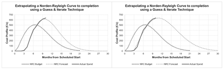
Figure 2.31 Extrapolating NRC to Completion Using the Guess and Iterate Technique (3)

Figure 2.32 Extrapolating a PERT-Beta Lookalike to Completion Using a Guess and Iterate Technique (1)
If instead we were to try to ‘Guess and Iterate’ values between these two we might conclude that the results in Figure 2.33 are better, and importantly that the range of outturn values for both cost and schedule have narrowed:
| Parameter | Left | Right |
| Start | 3 | 3 |
| End | 25.5 | 27 |
| Outturn | € 7,000 k | € 7,100 k |

Figure 2.33 Extrapolating a PERT-Beta Lookalike to Completion Using a Guess and Iterate Technique (2)
However, there is both a risk and an opportunity in the psychology of using this technique (with either an NRC or PERT-Beta.) There is a risk that we tend to iterate with fairly round numbers and miss the better fit that we might get by using more precise values for the three parameters. Paradoxically, therein lies the opportunity. We avoid going for the perfect best fit answer because we know that life doesn’t work that way; performance will change so we should not delude ourselves into sticking unswervingly to the current trend as the absolute trends do and will change, and consequently, so will the EAC. What we should be looking for is some stability over time.
2.6.2 Norden-Rayleigh Curve fitting with Microsoft Excel Solver
This technique will give us that more precise, albeit not necessarily more accurate result. The main benefit over ‘Guess and Iterate’ is its speed and repeatability. Appropriateness and Explicitness comes in the definition of any constraints we choose to impose, thus meeting our TRACEability paradigm.
In Table 2.16 we show a Model Set-up that allows Microsoft Excel’s Solver to vary the Start, Endpoint and Cost Outturn by minimising the Sum of Squares Errors

Table 2.16 Solver Model Set-Up for Norden-Rayleigh Curve Forecast
between the Actual Cumulative Spend and the Cumulative NRC Forecast Model. We have some options for the constraints that we choose to impose. Generally we would expect to set the constraint that the Sum of the Errors should be zero in line with usual practice for Least Squares Error, but there are occasions where we will get a ‘better fit’ if we relax that constraint, especially if we feel that there is already inherent bias in the model towards the Start point. We can also exercise our judgement to limit the range of possible values for Solver to consider in terms of the parameters; for instance, in this case we might want to specify that the Start point must be no less than 2 … and again we shouldn’t forget to untick the box marked ‘Make Unconstrained Values Non-negative’. Here, we have taken the starting parameter guesses to be the budget parameters; the results shown in Table 2.17 and Figure 2.34 relate to those in which the Sum of Errors is zero.

Table 2.17 Solver Model Results for Norden-Rayleigh Curve Forecast

Figure 2.34 Extrapolating a NRC to Completion Using Microsoft Excel’s Solver (1)
This gives us an Outturn value of € 6,777 k based on a Start point at month 2.86 and an Endpoint at month 25.74 (with a Mode at month 9.4).
We may recall from the previous technique that whilst we had what appeared to be a good fit to the cumulative profile, when we looked at it from a monthly perspective, it was not such a good result. Solver will overcome this in general, if it can, as illustrated in Figure 2.35.
Let’s see what happens if we use Solver with the NRC PERT-Beta lookalike. The model set-up is similar to the above but uses a BETA.DIST function instead with fixed parameters and . The Solver variable parameters are as before, and our Solver results are shown in Figures 2.36 and 2.37, and are based on the following parameters:
Start = 2.88 End = 27.51 Outturn = € 7,697 k
This result also appears to be an excellent fit to the data from both a cumulative and monthly burn rate perspective. However, it is fundamentally different to the forecast to completion created using the ‘pure’ Norden-Rayleigh Curve Solver model. Not only is it different, but it is substantially different! (Put that bottom lip away and stop sulking.) Let’s look at why and how we can use this to our benefit rather than detriment.

Figure 2.35 Extrapolating a NRC to Completion Using Microsoft Excel’s Solver (2)

Figure 2.36 Extrapolating a PERT-Beta Lookalike to Completion Using Microsoft Excel’s Solver (1)

Figure 2.37 Extrapolating a PERT-Beta Lookalike to Completion Using Microsoft Excel’s Solver (2)
If we recall from Figure 2.21 in Section 2.3.1, we saw the PERT-Beta Distribution was an excellent substitute for a Norden-Rayleigh Curve. However, in Figure 2.22 in Section 2.3.2 we showed that whilst the mode occurs in the same place there is a difference in the Probability Density Functions of the two distributions. The PERT-Beta has a slightly smaller Modal height, which is compensated for elsewhere. As our actuals are only available until around the Mode this will create a measurable difference between the two models. Look on the bright side … we now have a range estimate; the Norden-Rayleigh Model gives us a more optimistic prediction in this position than the PERT-Beta lookalike.
Once we get past the mode, things should begin to stabilise more and the gap will begin to narrow (assuming that this is a development project that follows the ‘rule’ of a single, bounded development as described in Section 2.1.4 to a reasonable extent).
2.6.3 Linear transformation and regression
Now from the look on some of our faces, we may be wondering how on Earth we can transform something like a Norden-Rayleigh Curve into straight line.
For the Formula-philes: Simple linear representation of a Norden-Rayleigh Curve
Consider a Norden-Rayleigh Curve generated from a Rayleigh Distribution with a Start point at time 0, a Mode at time λ and a nominal completion time at time τ, giving an uplift factor of k relative to the corresponding Rayleigh Distribution, in order to get an Outturn Cost of CT

Therefore, we can say that the Natural Log of the Rayleigh Distribution Estimate To Infinity is a linear function of the Square of Time Elapsed and the Rayleigh Distribution Estimate At Infinity.
The problem seems to be that we need to know the outturn value in order to perform the transformation … in other words, if we knew the answer then we would be able to solve the problem … which all seems a bit of a pointless circular argument because if we knew the answer then we wouldn’t have a problem. It isn’t just me, is it?
However, before we throw our arms in the air in despair, let’s take a step back; all is not lost. Microsoft Excel’s Solver can come to our rescue again! In Table 2.18 we show a possible model setup.

Table 2.18 Solver Model Setup for Linear Transformation of a Norden-Rayleigh Curve
- The left-hand three columns allow us to profile the budget of € 5,000 k as a Norden-Rayleigh Curve commencing at month 0 with a Mode at month 6, giving a nominal endpoint at month 21. In Microsoft Excel this is based on the Rayleigh Distribution as a special case of the Weibull Distribution with parameters of 2 and Mode √2 multiplied by an uplift factor of 100.219%, derived from the Truncation Ratio of 3.5
- The fourth column shows the actuals to date
- The header section of the next two columns depict the Solver starting parameters for our Solver model to determine the Best Fit Norden-Rayleigh Curve through the actuals. Here we have taken the budget values for the Start point, Mode and Outturn, although we could have picked any non-negative values at random
- The NRC Outturn multiplied by the Uplift Factor gives us our theoretical Rayleigh Distribution Estimate At Infinity (RD-EAI), shown as € 5,011 k in the example
- We can calculate the new variable ‘s’ as the square of the time from commencement, i.e. the actual month number minus the actual start parameter (not necessarily zero once Solver begins its iterations)
- We can determine the error between Actuals and the current ‘Best Fit’ Model allowing errors to be generated where the month is less than the Starting month parameter. (Errors will be generated when the ‘Time from Start’ value is less than zero.) We will exploit this in Step 8
- The Rayleigh Distribution Estimate To Infinity column (RD-ETI) is calculated by taking the RD-EAI minus the Actuals to date. We can then take the Natural Log of this in the next column
- Above these we can now calculate the number of points we should be using in the Regression step; this is simply the number of points which do not generate an error in Step 5. We do this by performing a simple count in Excel using the COUNT(range) function as it will ignore errors generated at Step 6
- Now this is the part where the Excel bit might get a bit stretching. We can now calculate the Regression Slope and Intercept using a combination of Excel Function SLOPE in conjunction with OFFSET, and also INTERCEPT in conjunction with OFFSET
- SLOPE(ETI-range, s-range) and INTERCEPT(ETI-range, s-range)
- ETI-range = OFFSET(Blank-ETI,-RegPoints,0,RegPoints,1)
- s-range = OFFSET(Blank-s,-RegPoints,0,RegPoints,1)
- Blank-ETI is the first blank cell immediately under the data range in column Natural Log Ln(RD-ETI)
- Blank-s is the first blank cell immediately under the data range in column Time from Start Squared (s)
- RegPoints is the number of valid regression points calculated in Step 8
Using the OFFSET function here allows us to count back the number of non-negative data points from Step 8 and creates an array or range one column wide and includes the number of rows defined by the number of Regression Points
- Using the calculated Slope of the regression line between time square variable 5 and Natural Log of RD-ETI, we can calculate the Offset Mode of the implied NRC as the reciprocal of (-2×Slope) .The cell RD-EAI can be calculated in Excel as EXP(Intercept) to reverse the transformation.
- The penultimate column is the Line of Best Fit using the calculated Intercept and Slope applied to the SquaredTime variable s, i.e. Intercept plus Slope multiplied by 5
- The final column expresses the difference between the 'actual' and Best Fit Ln(RD-ETI) columns, i.e. the error terms
- We can then calculate the Sum of these error values (which should always be zero as we have forced a regression through the data ... if they are not, we need to check our model out for mistakes). We can determine the Sum of Squares Errors (SSE) using SUMSQ in conjunction with OFFSET
- SUMSQ(Error-range )
- Error-range = OFFSET(Blank-Error,- RegPoints,0, RegPoints,1)
- Blank-Error is the first blank cell immediately under the data range in the end column
- RegPoints is the number of valid regression points calculated in Step 8
- No w for a little trick to make Excel Solver work that little bit harder for us. SSE is our Solver objective to minimise, but it will only try to minimise to a specified number of decimal places. As we are dealing with relatively small numbers with the Natural Log of the error values, we can force a more stringent convergence requirement in the Solver options … or we can take the lazy option and simply multiply the SSE by a fixed large number, like a million. (‘ Efficiency is intelligent laziness’ as they say)
- Finally, we can set up our Solver model using the inflated SSE as the objective to minimise by varying the Start, Mode and Outturn parameters subject to the following constraints:
- The two calculations in the header section for the theoretical Rayleigh Distribution Estimate At Infinity, RD-EAI, are the same (i.e. fifth column and the last column, highlighted by chevrons)
- The calculated Mode based on the Regression Slope equals the Solver input variable (sixth column and last column of the header section, highlighted by chevrons)
- The Outturn is greater than or equal to the actuals to date
- The Project Endpoint is greater than current month for which we have actual data
Ensure that the ‘Make Unconstrained Variables Non-negative’ option is not selected
We can now run Solver … only to find that it fails to converge in this instance. (Now, now, there’s no need to use language like that! ) Solver is an algorithm and works by incrementing its parameter values up to a maximum number of iterations. If we start it off too far away from the optimum solution, or point it in the wrong direction, then it may fail to converge, as it has here!
However, as the familiar adage advises, let’s try again with different starter values. A simple look at the data would suggest that the project has started around 3 months late, so we can try using that as an alternative starting parameter. We can also try moving the Mode by the same amount from month 6 to month 9. Let’s just increase the outturn randomly to € 6,000k, before trying again…
A word (or two) from the wise?
'If at first you don't succeed, Try, try, try again.'
William E Hickson
British Educational Writer
1803-1870
… and as if by magic, it now converges to the result in Table 2.19 and Figure 2.38 giving us a start month of 2.84, a Mode midway through month 10 (i.e. 9.581) and an outturn EAC of € 6,986 k.
If the false start has shaken your confidence in Solver, then try running it again several times using different input parameter values for start, mode and outturn. Hopefully this will return more consistent results, unless the actuals are not fitting a Norden-Rayleigh Curve pattern, in which case the transformation and regression are not valid.
The next question an enquiring estimator is bound to ask is ‘How stable is this EAC?’ Well, that’s a good question! Let’s add a couple of months’ worth of data and re-run the model. We get the results in Table 2.20 and Figure 2.39, which give us a similar start position, but a slightly later mode and an increased EAC outturn.
In fact, if we were to track the EAC and projected completion date, we would find a pattern emerging, as shown in Table 2.21 and Figure 2.40. In this particular case we can see that as the schedule slips each month the cost outturn also increases at a rate greater than the Pro Rata Product Rule (Section 2.2.3) but less than the Square Rule (Section 2.2.4) and that the average of the two is a very close approximation to what has happened here. We can imply therefore that the cost outturn increases in line with a general quadratic relationship in relation to schedule slippage in this instance; we should not infer that this will always be the case and should not use this as justification for fitting a quadratic curve of best fit to the Norden-Rayleigh Cost Creep Trend Analysis in Figure 2.41; if we did it would turn back on itself!

Table 2.19 Solver Model Results for Linear Transformation of a Norden-Rayleigh Curve (1)

Figure 2.38 Solver Model Results for Linear Transformation of a Norden-Rayleigh Curve (1)

Table 2.20 Solver Model Results for Linear Transformation of a Norden-Rayleigh Curve (2)
Now, as promised at the start of Section 2.6, we will return to the suggestion of Christensen and Rees (2002) that EVM systems can be used to predict EACs after they have reached the 20% completion level. This example shows that this may not be the case. The outturn prediction only starts to stabilise until we’re safely past the Mode, which is at around 40% completion, and in this particular case we are in excess of 50% of the predicted trend! Let’s just agree that it may be possible to get a stable view of a NRC EAC at a relatively early stage, but let’s not bank on it; we should track it regularly.
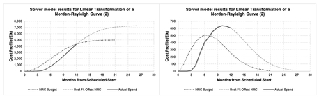
Figure 2.39 Solver Model Results for Linear Transformation of a Norden-Rayleigh Curve (2)

Table 2.21 Solver Outturn Creep Follows the Average of the Two Schedule Slippage Cost Rules

Figure 2.40 Solver Outturn Creep Follows the Average of the Two Schedule Slippage Cost Rules

Figure 2.41 Solver Outturn Creep Trend Analysis
2.6.4 Exploiting Weibull Distribution's double log linearisation constraint
This technique is essentially a variation on that discussed in the last section, exploiting the same basic property.
If we look back at Volume II Chapter 4 on the properties of Weibull Distributions we will find that we can transform any Weibull Distribution into a Linear Function using a double Natural Log. As a Norden-Rayleigh Curve is based on the Rayleigh Distribution which is just a special case of a Weibull Distribution, then the same must be true of a NRC.
For the Formula-philes: Alternative linear representation of a Norden-Rayleigh Curve
Consider a Norden-Rayleigh Curve generated from a Rayleigh Distribution with a Start point at time 0, a Mode at time λ and a nominal completion time at time τ, giving an uplift factor of k relative to the corresponding Rayleigh Distribution, and an Outturn Cost of CT

The relationship can be expressed as the:
Double Natural Log of the Underpinning Rayleigh Distribution’s Cumulative Percentage to Completion is a linear function of the Natural Log of the Elapsed Time
… which admittedly doesn’t quite flow off the tongue too readily.
In other words, this is another of those ‘we need to know the answer, to get the answer’, but as we have already seen in the previous section, Microsoft Excel’s Solver can help us to get around that one.
It has the property that the slope of this transformation is always 2, and that the Intercept is always -2 LN (Mode √2).
Table 2.22 and Figure 2.42 illustrate the transformation with a ‘perfect’ Norden-Rayleigh Curve:
- The outstanding Rayleigh Distribution % is 100% minus Column (A)
- Column (F) is the reciprocal of Column (E)
- Column (G) is the Natural Log of the Natural Log of Column (F), i.e. LN(LN(Column F))

Table 2.22 Transformation of a ‘Perfect’ Norden-Rayleigh Curve to a Linear Form
The slope of the transformation is always 2, and the intercept is always -2 LN (Mode √2).
However, by way of verification that the double Log Transformation is working, we have also shown these values calculated using the Excel functions SLOPE and INTERCEPT using range (G) as the known-y’s and range (D) as the known-x’s.

Figure 2.42 Transformation of a ‘Perfect’ Norden-Rayleigh Curve to a Linear Form
Now let’s try exploiting this property using our example actual data we considered in the previous three techniques. We are going to use Solver to find the Best Fit Norden-Rayleigh Curve to the actual data, but with the added constraint that exploits this Double Log linear transformation property. Table 2.23 illustrates an appropriate set-up procedure.
- The left-hand three columns set-up the Budget Norden-Rayleigh Curve as a reference
- The Actual costs to date are in the fourth column
- The fifth column header holds the parameter values for our intended ‘Best Fit’ NRC model. The Start point, Mode and Outturn Cost (EAC) will be used as the Solver variables but initially can be set at random. Here we have assumed that they are the Budget values
- The lower section of the fifth column offsets the Time (Months) by the Start point value (initially zero offset)
- The sixth column header summarises the revised Start and Mode parameters that will be used in the revised NRC calculation (i.e. they are normalised to reflect a start time of zero). It also multiplies the Outturn parameter by the Uplift Factor we have chosen to apply. Here we are assuming the 3.5 Truncation Ratio discussed previously. This gives us the theoretical cost at infinity required for the underlying Rayleigh Distribution which we will use in Steps 6 and 9

Table 2.23 Solver Setup Exploiting the Linear Transformation Property of a Norden-Rayleigh Curve
- The lower section of the sixth column depicts the revised NRC as defined above. Initially, as we have assumed the budget parameters, this column is identical to the third column (although it won’t be when Solver starts to run)
- The seventh column calculates the error between the Actual Cumulative Cost and the revised NRC. It summarises the Sum of Squares Error (or SSE); this is the value which we will get Solver to minimise, i.e. our usual Least Squares technique
- The last four columns are a repeat of the logic used in Table 2.22. In the header section we have calculated the Linear Transformation Intercept based on the revised Mode as -2 multiplied by the natural log of the revised mode and the square root of 2.
- In the lower section of these four columns we perform the linear transformation of the revised NRC using the double natural log of the reciprocal of the outstanding Rayleigh Distribution percentage. The important thing to note here is that the outstanding Rayleigh Distribution percentage in the column marked (E) is calculated by taking the Outturn (€ 5,000 k as the starting value in this case) minus the Actuals divided by the Outturn multiplied by the uplift factor. (Although in practice it makes little difference to the result)
- We can then determine the number of data points that we should use in our regression calculation of the slope and intercept of this linear transformation. If the revised start time is less than 1, we have chosen to exclude this from the regression. Values less than 1 generate negative natural log values, usually associated with a comparatively small cumulative cost. This in turn can create a distorted view of the transformation resulting in wildly inflated or deflated outturn values, as shown in Figure 2.43; this particular fit gives an EAC in excess of € 13,000 k! (Now you might think that this ‘random’ exclusion sounds very naughty but it is done from a pragmatic perspective, but I note your concern)
- Depending on the value of the Start point parameter the number of Regression Points to include will change dynamically within Solver. To avoid a failure to converge error, the number of Regression Points to include can be determined by taking the minimum of COUNTIF(range(D),’>0’) and COUNTIF(range(F),’>1’). The latter avoids an error value in column denoted as (G) by taking the Double Natural Logarithm of 1 as LN(1)=0, so LN(LN(1)) gives an #NUM error
- Next we calculate the slope and intercept of the linear transformation using the selected data points and the Microsoft Excel functions SLOPE(y-range, x-range) and INTERCEPT(y-range, x-range) where the y-range is in the column denoted as (G) and the x-range is in that denoted as (D)
- As the number of Regression Points to include will vary according to Step 10, we can use the OFFSET function in conjunction with SLOPE and INTERCEPT for the y-range and x-range

Figure 2.43 Distortion of the Linear Transformation of a NRC due to Negative Log Values
- y-range = OFFSET(G-Blank, -Regression Points, 0, Regression Points, 1) where G-Blank is the blank cell below the last data point in column denoted (G)
- x-r ange = OFFSET(D-Blank, -Regression Points, 0, Regression Points, 1) where D-Blank is the blank cell below the last data point in column denoted (D)
- The OFFSET function then counts back the number of non-negative data points from Step 10 and creates an array or range one column wide and includes the number of rows defined by the number of Regression Points
- We can now set up the Excel Solver to minimise the Sum of Squares Error value subject to the constraints that the Slope must be 2 (initially 4.8120), and the two intercept calculations must be equal also (initially they are 4.814 and -10.7986.) It is also a good idea to tell Solver that the Endpoint must be greater than ‘time now’ and that the outturn must be greater than the Actual cost to date, just to avoid it scooting off in the wrong direction and failing to converge
- Finally, let’s not forget to uncheck the box that forces all unconstrained parameters to be non-negative!

Table 2.24 Solver Results Exploiting the Linear Transformation Property of a Norden-Rayleigh Curve (1)
Clicking ‘Solve’ will yield us results similar to those in Table 2.24. This gives us an Outturn or EAC of some € 6,205 k and a completion date just after the end of Month 24, having started just before the end of month 3, and reaching a Mode at month 9 (and a bit). Figure 2.44 illustrates the result. It appears to be a reasonably good cumulative fit (left-hand graph) but the right-hand graph depicting the monthly spend suggests that the Modal value has been understated, relatively speaking.

Figure 2.44 Extrapolating a NRC to Completion Using a Transformation and Regression Technique (1)

Table 2.25 Solver Results Exploiting the Linear Transformation Property of a Norden-Rayleigh Curve (2)
If we re-run the model two months later as we did with the basic Least Squares Solver technique in the last section, we again get a different result, as shown in Table 2.25 and Figure 2.45. With an Outturn of € 6,826 k with a completion date midway through Month 26, having commenced just before the end of month 3. Worryingly, however, these values are significantly lower than those generated by the previous technique; also, we will note that the right-hand graph of Figure 2.45 suggests that the programme is likely to slip even more with a knock-on to costs. Whilst this technique exploits a property of the Rayleigh Distribution, it does pre-suppose that the model is true in an absolute sense, which may be a somewhat misplaced reliance. (After all, since when did anything to do with estimating become an exact science?)

Figure 2.45 Extrapolating a NRC to Completion Using a Transformation and Regression Technique (2)

Table 2.26 Solver Outturn Creep Follows a Weighted Average of the Two Schedule Slippage Cost Rules
In Table 2.26 and Figure 2.46 we can track the performance of this technique over time and there appears to be little convergence to a steady state condition. This technique may suffer from an over reliance on a model which is really only an empirical observation that employs a truncation rule in order to work. The mere fact that we had to interject a fairly random step of ignoring negative Log Values should have warned us that pragmatic decisions are not always practical decisions.

Figure 2.46 Solver Outturn Creep Trend Analysis
Our conclusion here must surely be that this may not be the most robust technique (or application of it). It seems to be a question of a good theory looking for a relevant problem to solve. Perhaps this is one to put in the ‘Don’t try this at home, or at work’ pile or may be one just to use as a sensitivity check value. In other situations, it may work a treat.
2.6.5 Estimates to Completion – Review and conclusion
As a refresher let’s compare the results of Period 10 and Period 12 across the four techniques and six answers. (We have two techniques that can be used with either the Norden-Rayleigh Curve or the PERT-Beta Lookalike.)
Table 2.27 summarises the results, and as we can see, there is a degree of variation in the values generated. Before we throw it all in the bin, let’s look on the bright side; we can use the various techniques to develop a range estimate as shown in Figure 2.47. If we were to continue the process with additional monthly updates, we would find (unsurprisingly) that the set of technique results are likely to continue to converge; this is a typical example of the Cone of Uncertainty (Volume I Chapter 4) articulated by Bauman (1958) and Boehm (1981) applied to the life of an Estimate to

Table 2.27 Comparison of Outturn Predictions Using Four Techniques
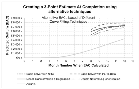
Figure 2.47 Creating a 3-Point Estimate at Completion Using Alternative Techniques
Completion. Here, we are progressively replacing and reducing uncertainty around future values with the certainty of actuals. The key thing for us here is to get over the hump, i.e. the mode (rather than get the hump over the differences). In this test, the PERT-Beta appears to be more likely to continue to give a slightly more pessimistic forecast, but generally appears to stabilise earlier, whereas the Double Natural Log Linearisation still tends to be understated. A combination of these techniques could be used to generate a 3-Point Estimate.
We mustn’t lose sight of the fact that the Norden-Rayleigh Curve is an empirical relationship, around which certain development behavioural characteristics have been postulated. If those characteristics do not describe our situation then we may find that none of these EAC/ETC techniques are appropriate. However, we may be able to use the general Least Squares Curve Fitting technique described in Volume III using either a general Weibull or, perhaps even better to avoid truncation issues, a general Beta Distribution. The Double Natural Log Linearisation Technique could be adapted for a general Weibull Distribution, but as we have seen with the Norden-Rayleigh Curve, it may be trying to enforce too exacting a constraint on what is after all only a representation of reality and not a physical law.
2.7 Chapter review
In this chapter we have looked at using Norden-Rayleigh Curves for Non-Recurring Development (or NRC4NRD).
We started by briefly reviewing its history and how Norden observed that spend patterns on Non-Recurring Development projects followed a Rayleigh Distribution. He postulated reasons why this was the case and expressed a number of conditions in which the empirical relationship was valid; the main one was that the development should be a self-contained development for which the final objective remains unchanged.
The main problem with a Rayleigh Distribution is that it goes on forever (sorry, did someone say, ‘Just like this chapter’?) Although some development projects may seem to be never-ending, we do need to have a practical limit on when the development is deemed to have been completed. There is no single view of when this should be; some choose the 97% Confidence Level as the truncation point giving a 2.65 ratio between the development Mode (peak effort) and the endpoint. Others prefer to use a 3.5:1 ratio between Mode and endpoint. The benefit of the latter is that it requires much less ‘adjustment’ to take account of premature truncation.
For those of us who are averse to random truncations, we can always consider using a PERT-Beta Distribution with parameters and . (Note that 7 is twice the NRC Truncation Ratio of 3.5, which may make it easier to remember.)
Whilst the NRC was originally conceived for projects that follow a natural development cycle unhindered, we can assess the impact when these ‘rules are broken’. This gives us some rule of thumb for schedule slippage such as the Pro Rata Product Cost Rule and the Square Cost Rule, depending on the reason for the slippage. We can also model phased developments by layering multiple Norden-Rayleigh Curves. Depending on the level and timing of the additional development tasks, we can get a Dromedary or Bactrian Camel effect. This ‘camelling’ effect might be suitably modelled as general Weibull or Beta Distributions. We might find also that in certain circumstances a phased development project may easily be mistaken for a pure Norden-Rayleigh single contained development project. In the scheme of things, it probably does not matter.
We ended our exploration into Norden-Rayleigh Curves by looking at potential techniques we can try to generate Estimates to Completion for existing Development projects. We could use a ‘Guess and Iterate’ technique, but that is prone to subjective opinion and fails our TRACEability paradigm. We could use a Least Squares Curve Fitting with either the Norden-Rayleigh Curve or the PERT-Beta Lookalike, the latter potentially giving a more pessimistic perspective than the NRC option.
If we exploit the properties of a Rayleigh Distribution (as a special case of the Weibull Distribution) and transform the Estimate To Completion into a linear format, we can then perform a linear regression. However, if we go for the Double Natural Log transformation of a Weibull Distribution then it appears to place too much of a purist constraint on what is after all an empirical relationship. As a consequence, this last technique may give spurious results until later in the project life cycle, and so is probably not the best option to use.
All this makes you wonder if the effort required by an organisation to pull together a major complex bid for new work, also follows a Norden-Rayleigh Curve? Now, who’s developing a headache? Time for a lie-down.
References
Amneus, D & Hawken, P (1999) Natural Capitalism: Creating the Next Industrial Revolution, Boston, Little Brown & Co, p.272.
Augustine, NR (1997) Augustine’s Laws (6th Edition), Reston, American Institute of Aeronautics and Astronautics, Inc.
Bauman, HC (1958) ‘Accuracy considerations for capital cost estimation’, Industrial & Engineering Chemistry, April.
Boehm, BW (1981) Software Engineering Economics, Upper Saddle River, Prentice-Hall.
Christensen, DS & Rees, DA (2002) ‘Is the CPI-based EAC a lower bound to the final cost of post A-12 contracts?’, The Journal of Cost Analysis and Management, Winter 2002.
Dukovich, J, Houser, S & Lee, DA (1999) The Rayleigh Analyzer: Volume 1 – Theory and Applications, AT902C1, McLean, Logistics Management Institute.
Gallagher, MA & Lee, DA (1996) ‘Final-Cost Estimates for research & development programs conditioned on realized costs’, Military Operations Research, Volume 2, Number 2: pp.51–65.
Fazar, W (1959) ‘Program evaluation and review technique’, The American Statistician, V olume 13, Number 2, April: p.10.
Lee, DA, Hogue, MR & Hoffman, DC (1993) Time Histories of Expenditures for Defense Acquisition Programs in the Development Phase. – Norden-Rayleigh and Other Models, ISPA Annual Meeting.
Lee, DA (2002) ‘Norden-Raleigh Analysis: A useful tool for EVM in development projects’, The Measurable News, Logistics Management Institute, March.
Norden, PV (1963) ‘Useful tools for project management’ in Dean, BV (Ed.) Operations Research in Research and Development, John Wiley and Sons.
Putnam, LH & Myers, W (1992) Measures for Excellence – Reliable Software on Time, within Budget, Upper Saddle River, Prentice-Hall.
Younossi, O, Stem, DE, Lorell, MA & Lussier, FM (2005) Lessons Learned from the F/A-22 and F/A-18 E/F Development Programs, Santa Monica, CA, RAND Corporation, [online] Available from: http://www.rand.org/pubs/monographs/MG276.html [Accessed 24–01–2017].