![]()
The Equities Market
Owning shares of company profits is one of the most common ways to invest and generate wealth. A large number of people who have made a fortune have achieved it by creating or buying an equity stake in a successful corporation. This is the reason the equity market is so popular among all kinds of investors. Moreover, the stock market is so vast that it provides opportunities for everyone willing to participate: from small investors to large hedge funds, you will find an investment style for each kind of participant.
The equities market is also an exciting area for software engineers, since it provides so many opportunities to apply computational techniques, which can be implemented in C++. Software engineers are also great allies to market analysts and investors in general, helping in vital activities such as modeling market data and devising algorithms needed to make fast and accurate trading decisions.
Due to their large size, equity markets are multifaceted and offer a huge variety of investment vehicles. From small cap stocks to blue chips, ETFs (exchange-traded funds), equity and index options, and other derivatives, there are a great number of opportunities for employing investment algorithms, in order to get an edge in the market. As a result, there is also great incentive (from banks and other investment institutions) to apply high-speed C++ programming techniques to solve such problems.
In this chapter we present C++ recipes for a few selected problems occurring in the equities markets and their derivatives. We will consider financial programming topics such as the following:
- Calculating simple moving averages.
- Computing exponential moving averages.
- Calculating volatility.
- Computing correlation of equity instruments.
- Modeling and calculating fundamental indicators.
The equity markets exist to expedite the trading of equity-based investments. The goal of an equity investment is to allocate money directly or indirectly to company stock, which gives buyers a certain share of ownership in a company. The idea behind this investment is to profit from the growth of the institution represented by that particular investment vehicle. For example, buying shares of IBM stock gives ownership of a small part of the company, along with the future profits associated with that ownership.
Direct stock ownership is the simplest example of an equity investment. Anyone with a brokerage account can buy shares in public companies, that is, companies that have put their shares for sale in the public market. Using their particular trading accounts or retirement accounts, individual investors have the ability to invest in any one of the thousands of publicly traded companies in the US and international markets.
However, directly controlling a company stock is not the only (or even the easiest) way to participate in the stock market. There are nowadays a plethora of products that offer alternative ways to invest in equity. This includes mutual funds, ETFs, index funds, options, and other more exotic derivatives. How to select the right instrument from such a large array of tradable issues is one of the many problems faced by money managers and individual investors.
Market Participants
The equities market is composed of many participants. They have different goals and interests; however, they work continuously to maintain market prices while trying to profit from them.
Large institutions form a sizable portion of the equities market landscape. These big, sell-side investment institutions (such as investment banks and exchanges) are viewed as the backbone of the market. Therefore, they are also commonly referred to as market makers. These large companies are buying and selling great volumes of equity investment vehicles (such as stocks) daily, with the goal of having small profits in each operation. More recently, high-frequency trading was added to this picture, resulting in increased volume and speed in market transactions.
Following is a quick list of the most common players in the equities market:
- Mutual funds: These funds receive investments from retail investors and institutions and make investments in areas of the market that they believe will have larger than usual investment returns. Mutual funds are mostly limited to buying stocks and ETFs, so their performance is limited when the market is in a downtrend.
- Hedge funds: Hedge funds use more advanced techniques, such as shorting stocks and buying options and futures, so they are limited to wealthier investors and some kinds of institutions that can cope with the increased risk.
- Investment banks: These institutions are actively working on the market composition. For example, they act in bringing to the market new issues (also known as IPOs) that will be traded by other investors. They are also allowed to trade for themselves and other large clients.
- High-frequency trading funds: These funds use high-performance computational techniques to provide instant liquidity to the markets, while making small profits in a large number of transactions.
- Brokerage companies: These companies work directly with individual investors providing the ability to buy or sell stocks, ETFs, mutual funds, and options for a small commission per transaction. Their services are made available through the Internet on several platforms such as desktops, web browsers, and mobile devices.
- Pension funds: These are institutions that hold large pools of investment money derived from retirement funds. They are geared toward long-term investments that will support the desired growth of the fund for an extended time period.
- Retail investors: These are individuals who control a brokerage account and do their own research and make their own decisions on what to buy and sell in the market.
As you can see, there is a great deal of competition for profits in the equities market. Most large institutions spend a lot of money on research that can give them an edge on the future moves of the market. This type of analytical approach depends on accurate information and instant access to trading data, which is possible only with the computational power provided by computer software, most of it written in languages such as C++.
In the next few sections I provide C++ recipes for common problems found in the analysis of equity investments. You will learn about tools and concepts that can be used in a large number of situations in which equity investments are involved.
Moving Average Calculation
Problem
Given a particular equity investment, determine the simple moving average and the exponential moving average for a sequence of closing prices.
Solution
One of the most common strategies to analyze equity instruments such as stocks and ETFs is to use supply/demand methods that consider price and volume as the important variables to observe. Traders who use price/volume-based strategies call this set of methods technical analysis (TA). With TA, traders look at special price points that have been defined by previous price movements, such as support, resistance, trend lines, and moving averages, with the objective of identifying pricing regions with a higher probability of profit.
For example, support and resistance values are typically used to determine price areas that are considered to be of importance for a given instrument. If a stock reaches a certain price when moving up and reverses course, the high price point is considered to be a resistance price. In the future, when the price again reaches the same area, traders will tend to sell around in the same region, creating an even stronger resistance point. Similarly, support prices are formed when traders buy the same stock or ETF in a well-known region.
A similar type of pattern occurs with moving averages. Buyers and sellers tend to look at moving averages to determine if a particular stock is on a low-risk buy or sell point. These psychological price points are self-reinforcing and play an important role in the dynamics of equity trading. Figure 2-1 shows an example of a moving average used in the analysis of common stock for Apple.
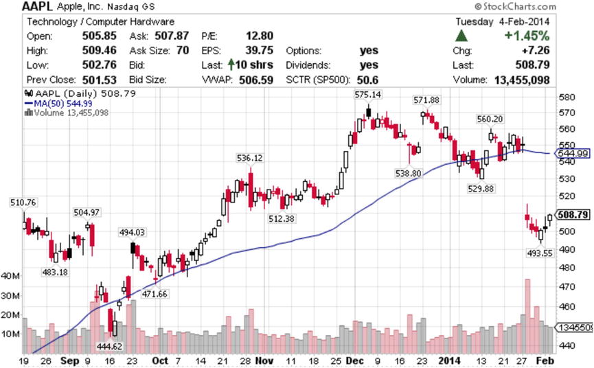
Figure 2-1. Simple moving average for daily prices of Apple (AAPL), with parameter 50
The moving average can be calculated using a simple average formula that is repeated for each new period. Given prices p1, p2, ..., pN, the general formula for a particular time period is given by
MA = (1/N) (p1 + p2 + ... + pN)
You can easily perform this calculation if you maintain and update the sequence of prices as new values are added to the sequence.
To calculate the moving average in C++, we first create a new class that stores a sequence of prices using a STL (standard templates library) vector object. The object is responsible for adding new values to the sequence, using the addPriceQuote member function. The implementation of this member function is simple because it relies on the functionality provided by std::vector to maintain a sequence of numbers, as well as the storage requirements.
void MACalculator::addPriceQuote(double close)
{
    m_prices.push_back(close);
}
The number of periods for moving average calculation is determined by the parameter to the constructor of the MACalculator class. For example, to compute a moving average for 20 time periods (normally the equivalent to four trading weeks when the period is a single trading day), you can create an object of the MACalculator class in the following way:
MACalculator calculator(20); // will compute the moving average for 20 periods.
The calculation of the simple moving average is performed by the calculateMA member function of the MACalculator class. The main idea of this function is to iterate through the sequence of prices stored in the MACalculator class, as shown in the following code:
std::vector<double> MACalculator::calculateMA()
{
    std::vector<double> ma;
    double sum = 0;
    for (int i=0; i<m_prices.size(); ++i)
    {
        sum += m_prices[i];
        if (i >= m_numPeriods)
        {
            ma.push_back(sum / m_numPeriods);
            sum -= m_prices[i-m_numPeriods];
        }
    }
    return ma;
}
To calculate a moving average, it is necessary to have at least the number of observations determined by the number of periods (let N be the number of periods). Therefore, the first N elements of the vector of prices don’t generate a corresponding moving average. These initial elements are simply added to the sum local variable, so their values are used later.
For each element after the Nth position, it is possible to calculate the moving average. This is achieved using the sum of the previous N elements and dividing it by the value N. The resulting value is appended to the vector of moving average elements. Finally, it is necessary to update the variable sum, so that the first item of the N-element sequence is dropped from the summation. This happens when the algorithm subtracts the value m_prices[i-m_numPeriods], preparing for the next iteration.
The exponential moving average (EMA) is different from the simple moving average because each new value is multiplied by a factor. This factor is used to give more weight to new values, as compared to older observations. As a result, the EMA is more responsive to changes in the observed values, and it can indicate new trends sooner and with better accuracy. This may be an advantage if you want to quickly spot changes in trend. Following is the code that I used:
std::vector<double> MACalculator::calculateEMA()
{
    std::vector<double> ema;
    double multiplier = 2.0 / (m_numPeriods + 1);

    // calculate the MA to determine the first element corresponding
    // to the given number of periods
    std::vector<double> ma = calculateMA();
    ema.push_back(ma.front());

    // for each remaining element, compute the weighted average
    for (int i=m_numPeriods+1; i<m_prices.size(); ++i)
    {
        double val = (1-multiplier) * ema.back() + multiplier * m_prices[i];
        ema.push_back(val);
    }
    return ema;
}
The initial part of the calculation is similar to the simple moving average. Values are added using the sum variable, until at least N values have been observed. This is used as the initial value for the EMA. Different implementations of EMA use other ways to initialize the sequence, but the results converge to the same values after a few iterations. You can see a graphical example of EMA in Figure 2-2.
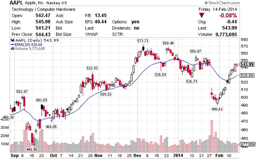
Figure 2-2. Exponential moving average with a parameter of 20 days
The main step of the EMA calculation is the addition of new values that are weighted by the multiplier. The default multiplier ρ for EMA computation is given by

This multiplier gives greater weight to new values, thus making the EMA more responsive to price changes than the simple moving average.
Complete Code
In Listing 2-1 you can see the complete implementation of the simple moving average as well as the EMA. I also show a sample main function that is responsible for reading a few data points from standard input and calculate the corresponding moving averages.
Listing 2-1. MACalculator
//
//  MACalculator.h

#ifndef __FinancialSamples__MACalculator__
#define __FinancialSamples__MACalculator__

#include <vector>

class MACalculator {
public:
    MACalculator(int period);
    MACalculator(const MACalculator &);
    MACalculator &operator = (const MACalculator &);
    ~MACalculator();

    void addPriceQuote(double close);
    std::vector<double> calculateMA();
    std::vector<double> calculateEMA();
private:
    // number of periods used in the calculation
    int m_numPeriods;
    std::vector<double> m_prices;
};

#endif /* defined(__FinancialSamples__MACalculator__) */

//
//  MACalculator.cpp

#include "MACalculator.h"

#include <iostream>

MACalculator::MACalculator(int numPeriods)
: m_numPeriods(numPeriods)
{

}

MACalculator::~MACalculator()
{

}

MACalculator::MACalculator(const MACalculator &ma)
: m_numPeriods(ma.m_numPeriods)
{

}

MACalculator &MACalculator::operator = (const MACalculator &ma)
{
    if (this != &ma)
    {
        m_numPeriods = ma.m_numPeriods;
        m_prices = ma.m_prices;
    }
    return *this;
}

std::vector<double> MACalculator::calculateMA()
{
    std::vector<double> ma;
    double sum = 0;
    for (int i=0; i<m_prices.size(); ++i)
    {
        sum += m_prices[i];
        if (i >= m_numPeriods)
        {
            ma.push_back(sum / m_numPeriods);
            sum -= m_prices[i-m_numPeriods];
        }

    }
    return ma;
}

std::vector<double> MACalculator::calculateEMA()
{
    std::vector<double> ema;
    double sum = 0;
    double multiplier = 2.0 / (m_numPeriods + 1);
    for (int i=0; i<m_prices.size(); ++i)
    {
        sum += m_prices[i];
        if (i == m_numPeriods)
        {
            ema.push_back(sum / m_numPeriods);
            sum -= m_prices[i-m_numPeriods];
        }
        else if (i > m_numPeriods)
        {
            double val = (1-multiplier) * ema.back() + multiplier * m_prices[i];
            ema.push_back(val);
        }
    }
    return ema;
}

void MACalculator::addPriceQuote(double close)
{
    m_prices.push_back(close);
}

//
//  main.cpp

#include "MACalculator.h"

#include <iostream>

// the main function receives parameters passed to the program
// and calls the MACalculator class
int main(int argc, const char * argv[])
{
    if (argc != 2)
    {
        std::cout << "usage: progName <num periods>" << std::endl;
        return 1;
    }

    int num_periods = atoi(argv[1]);

    double price;
    MACalculator calculator(num_periods);
    for (;;) {
        std::cin >> price;
        if (price == -1)
            break;
        calculator.addPriceQuote(price);
    }

    std::vector<double> ma = calculator.calculateMA();

    for (int i=0; i<ma.size(); ++i)
    {
        std::cout << "average value " << i << " = " << ma[i] << std::endl;
    }

    std::vector<double> ema = calculator.calculateEMA();

    for (int i=0; i<ema.size(); ++i)
    {
        std::cout << "exponential average value "
            << i << " = " << ema[i] << std::endl;
    }

    return 0;
}
Running the Code
You can compile this code using the gcc compiler (as well as any other standards-compliant compiler such as Visual Studio or C++ builder). For example, the following command line can be used from the UNIX shell:
gcc -o macalc main.cpp macalculator.cpp
Following is a display of a sample execution of the program:
$ ./macalc 5
10
11
22
12
13
23
12
32
12
3
2
22
32
-1
average value 0 = 18.2
average value 1 = 18.6
average value 2 = 22.8
average value 3 = 20.8
average value 4 = 19
average value 5 = 16.8
average value 6 = 16.6
average value 7 = 20.6
exponential average value 0 = 18.2
exponential average value 1 = 16.1333
exponential average value 2 = 21.4222
exponential average value 3 = 18.2815
exponential average value 4 = 13.1877
exponential average value 5 = 9.45844
exponential average value 6 = 13.639
exponential average value 7 = 19.7593
Program ended with exit code: 0
In the first line, I entered the command that calls the moving average program (which here is simply called macalc). The single argument in the command line means that I want to calculate the moving average for five data points. Then, I entered a sequence of numbers that represents the observed prices for a certain investment vehicle. Finally, I entered the value -1, which indicates the end of the input. The next few lines then give a list of values that define the simple moving average and the EMA.
Problem
Calculate the volatility of a particular equity instrument, given a sequence of prices for the last few days.
Solution
One of the important characteristics of stocks and other equity instruments is that they change in price very frequently. For highly liquid stocks and ETFs, prices will change during the whole trading day, as new buyers and sellers exchange shares. The result is a high degree of volatility, as compared to other investment instruments.
Volatility is also an important concept when comparing investment options. For example, an Internet stock will vary in price much more widely than a traditional food producer. Their volatility profiles will be completely different. Higher volatility may be an advantage or a disadvantage, depending on your investment objectives.
The important thing to consider about volatility is that it is not just a one-dimensional concept. Different investment strategies require different ways of viewing price variations. For example, if you are making investment decisions based on the expected volatility for the next few days (due to a news event or earnings release), then the previous week’s volatility may not be so important.
In this section, I present three ways to measure volatility given a sequence of prices. The first strategy is computing the range of values observed during that period. This is probably the simplest way to view volatility: calculate the highest and lowest observed values and return its difference. It is also a common indicator used by many investors. Most newspapers print a list of one-year high and low prices, so you can quickly see the simple range for the previous year. Following is the implementation using a vector of prices:
double VolatilityCalculator::rangeVolatility()
{
    if (m_prices.size() < 1)
    {
        return 0;
    }

    double min = m_prices[0];
    double max = min;
    for (int i=1; i<m_prices.size(); ++i)
    {
        if (m_prices[i] < min)
        {
            min = m_prices[i];
        }
        if (m_prices[i] > max)
        {
            max = m_prices[i];
        }
    }
    return max - min;
}
The second strategy is calculating the average range for a given time period. For example, many investment strategies use the idea of looking at the past few days and taking an average of the observed ranges. The result is then charted as an indicator of the rate of change for a particular stock, for example. Simply calculating the average of the previously observed daily ranges can be used to return this value. Here is our code.
double VolatilityCalculator::avgDailyRange()
{
    unsigned long n = m_prices.size();
    if (n < 2)
    {
        return 0;
    }

    double previous = m_prices[0];
    double sum = 0;
    for (int i=1; i<m_prices.size(); ++i)
    {
        double range = abs(m_prices[i] - previous);
        sum += range;
    }
    return sum / n - 1;
}
Finally, a more sophisticated way to gauge the variation of values for an equity instrument is to use the statistical definition of standard deviation. The standard deviation is useful as a way to derive volatility from the expected value (also known as mean) of a set of prices. A well-known formula is used to calculate the standard deviation, which is given by
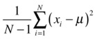
In this equation, N is the number of data points (prices) and μ is the average of these values. The standard deviation can be calculated in C++ with the following code:
double VolatilityCalculator::stdDev()
{
    double m = mean();
    double sum = 0;
    for (int i=0; i<m_prices.size(); ++i)
    {
        double val = m_prices[i] - m;
        sum += val * val;
    }
    return sqrt(sum / (m_prices.size()-1));
}
Complete Code
Listing 2-2 provides the complete code for the strategies just described. I introduce a new C++ class named VolatilityCalculator, which encapsulates the concept of computing the price volatility. We have these three strategies coded in the rangeVolatility, avgDailyRange, and stdDev member functions. You can use this class as a starting point, and later add other methods for volatility calculation as additional member functions.
Listing 2-2. VolatilityCalculator.h
//
//  VolatilityCalculator.h

#ifndef __FinancialSamples__VolatilityCalculator__
#define __FinancialSamples__VolatilityCalculator__

#include <vector>

class VolatilityCalculator
{
public:
    VolatilityCalculator();
    ~VolatilityCalculator();
    VolatilityCalculator(const VolatilityCalculator &);
    VolatilityCalculator &operator=(const VolatilityCalculator &);

    void addPrice(double price);
    double rangeVolatility();
    double stdDev();
    double mean();
    double avgDailyRange();
private:
    std::vector<double> m_prices;
};

#endif /* defined(__FinancialSamples__VolatilityCalculator__) */

//
//  VolatilityCalculator.cpp

#include "VolatilityCalculator.h"

#include <iostream>
#include <cmath>

VolatilityCalculator::VolatilityCalculator()
{

}

VolatilityCalculator::~VolatilityCalculator()
{

}

VolatilityCalculator::VolatilityCalculator(const VolatilityCalculator &v)
: m_prices(v.m_prices)
{

}

VolatilityCalculator &VolatilityCalculator::operator =(const VolatilityCalculator &v)
{
    if (&v != this)
    {
        m_prices = v.m_prices;
    }
    return *this;
}

void VolatilityCalculator::addPrice(double price)
{
    m_prices.push_back(price);
}

double VolatilityCalculator::rangeVolatility()
{
    if (m_prices.size() < 1)
    {
        return 0;
    }

    double min = m_prices[0];
    double max = min;
    for (int i=1; i<m_prices.size(); ++i)
    {
        if (m_prices[i] < min)
        {
            min = m_prices[i];
        }
        if (m_prices[i] > max)
        {
            max = m_prices[i];
        }
    }
    return max - min;
}

double VolatilityCalculator::avgDailyRange()
{
    unsigned long n = m_prices.size();
    if (n < 2)
    {
        return 0;
    }

    double previous = m_prices[0];
    double sum = 0;
    for (int i=1; i<m_prices.size(); ++i)
    {
        double range = abs(m_prices[i] - previous);
        sum += range;
    }
    return sum / n - 1;
}

double VolatilityCalculator::mean()
{
    double sum = 0;
    for (int i=0; i<m_prices.size(); ++i)
    {
        sum += m_prices[i];
    }
    return sum/m_prices.size();
}

double VolatilityCalculator::stdDev()
{
    double m = mean();
    double sum = 0;
    for (int i=0; i<m_prices.size(); ++i)
    {
        double val = m_prices[i] - m;
        sum += val * val;
    }
    return sqrt(sum / (m_prices.size()-1));
}

//
//  main.cpp

#include "VolatilityCalculator.h"

#include <iostream>

// the main function receives parameters passed to the program
int main(int argc, const char * argv[])
{
    double price;

    VolatilityCalculator vc;
    for (;;)
    {
        std::cin >> price;
        if (price == -1)
        {
            break;
        }
        vc.addPrice(price);
    }

    std::cout << "range volatility is " <<  vc.rangeVolatility()  << std::endl;
    std::cout << "average daily range is " <<  vc.avgDailyRange()  << std::endl;
    std::cout << "standard deviation is " <<  vc.stdDev()  << std::endl;
    return 0;
}
Running the Code
Here is an example of the volatility class being used. You can compile the code presented in Listing 2-2, assuming that the binary is called volatility. Then, you can use the program by entering price values that will be later used to compute the volatility employing the three methods described. The end of the input sequence is determined by a single -1 value entered as the last input value.
$ ./volatility
3
3.5
5
4.48
5.2
6
6.1
5.5
5.2
5.7
-1
range volatility is 3.1
average daily range is 0.7
standard deviation is 1.02957
Computing Instrument Correlation
Problem
Given a sequence of closing prices for the last N periods, calculate the correlation between two equity instruments.
Solution
One of the main problems that money managers need to solve is how to diversify a portfolio. The problem of diversification occurs because, when investing in the market, it is not desirable to have all your assets in the same type of investment. Correlated investments tend to go down at the same time, making it harder to avoid losses in a portfolio.
For example, consider two companies operating in a similar business. The classic example is beverage companies such as Coca-Cola and Pepsi. They tend to rise and fall at the same time due to the similarity of their business. Therefore, we say that they are highly correlated. Correlation is a mathematical concept that was developed for the analysis of statistical events. It turns out to be an important concept in the equities market, since probability plays such a big role in the evaluation and modeling of equity-based investments.
To make the code for this example more extensible, we divide the solution into two classes. The first class, called TimeSeries, represents the often-used concept of a set of numbers that apply to a certain quantity over a given period of time. This concept is commonly referred to as a time series. The TimeSeries class is responsible for calculating values that are specific to a single time series, such as the average, or the standard deviation.
The second class used is CorrelationCalculator, which is responsible for collecting data for the desired time series and computing the correlation using the formula
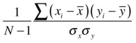
In this equation, N is the number of observations, xi is the i-th observation of the first time-series, yi is the i-th observation of the second time-series, ![]() and
and ![]() are the mean (average) of the two sequences of prices, sx is the standard deviation of the x values, and sy is the standard deviation of the y values.
are the mean (average) of the two sequences of prices, sx is the standard deviation of the x values, and sy is the standard deviation of the y values.
The mean value and the standard deviation are calculated in the TimeSeries class. These values are then used in the CorrelationCalculator to determine the correlation between the values observed for both sequences.
Complete Code
The computation discussed in the previous section is implemented in the class TimeSeries. Listing 2-3 includes the complete class. You can also see how to use techniques to calculate correlation, as displayed in the class CorrelationCalculator.
Listing 2-3. TimeSeries.h
//
//  TimeSeries.h

#ifndef __FinancialSamples__TimeSeries__
#define __FinancialSamples__TimeSeries__

#include <vector>

class TimeSeries
{
public:
    TimeSeries();
    TimeSeries(const TimeSeries &);
    TimeSeries &operator=(const TimeSeries &);
    ~TimeSeries();

    void addValue(double val);
    double stdDev();
    double mean();
    size_t size();
    double elem(int i);
private:
    std::vector<double> m_values;
};

#endif /* defined(__FinancialSamples__TimeSeries__) */

//
//  TimeSeries.cpp

#include "TimeSeries.h"
#include <cmath>
#include <iostream>

TimeSeries::TimeSeries()
: m_values()
{

}

TimeSeries::~TimeSeries()
{

}

TimeSeries::TimeSeries(const TimeSeries &ts)
: m_values(ts.m_values)
{
}

TimeSeries &TimeSeries::operator =(const TimeSeries &ts)
{
    if (this != &ts)
    {
        m_values = ts.m_values;
    }
    return *this;
}

void TimeSeries::addValue(double val)
{
    m_values.push_back(val);
}

double TimeSeries::mean()
{
    double sum = 0;
    for (int i=0; i<m_values.size(); ++i)
    {
        sum += m_values[i];
    }
    return sum/m_values.size();
}

double TimeSeries::stdDev()
{
    double m = mean();
    double sum = 0;
    for (int i=0; i<m_values.size(); ++i)
    {
        double val = m_values[i] - m;
        sum += val * val;
    }

    return sqrt(sum / (m_values.size()-1));
}

size_t TimeSeries::size()
{
    return m_values.size();
}

double TimeSeries::elem(int pos)
{
    return m_values[pos];
}

//
//  CorrelationCalculator.h

#ifndef __FinancialSamples__CorrelationCalculator__
#define __FinancialSamples__CorrelationCalculator__

class TimeSeries;

class CorrelationCalculator
{
public:
    CorrelationCalculator(TimeSeries &a, TimeSeries &b);
    ~CorrelationCalculator();
    CorrelationCalculator(const CorrelationCalculator &);
    CorrelationCalculator &operator =(const CorrelationCalculator &);

    double correlation();
private:
    TimeSeries &m_tsA;
    TimeSeries &m_tsB;
};

#endif /* defined(__FinancialSamples__CorrelationCalculator__) */

//
//  CorrelationCalculator.cpp

#include "CorrelationCalculator.h"

#include "TimeSeries.h"
#include <iostream>

CorrelationCalculator::CorrelationCalculator(TimeSeries &a, TimeSeries &b)
: m_tsA(a),
  m_tsB(b)
{
}

CorrelationCalculator::~CorrelationCalculator()
{

}

CorrelationCalculator::CorrelationCalculator(const CorrelationCalculator &c)
: m_tsA(c.m_tsA),
  m_tsB(c.m_tsB)
{

}

CorrelationCalculator &CorrelationCalculator::operator=(const CorrelationCalculator &c)
{
    if (this != &c)
    {
        m_tsA = c.m_tsA;
        m_tsB = c.m_tsB;
    }
    return *this;
}

double CorrelationCalculator::correlation()
{
    double sum = 0;
    double meanA = m_tsA.mean();
    double meanB = m_tsB.mean();

    if (m_tsA.size() != m_tsB.size()) {
        std::cout << "error: number of observations is different" << std::endl;
        return -1;
    }

    for (int i=0; i<m_tsA.size(); ++i)
    {
        auto val = (m_tsA.elem(i) - meanA) * (m_tsB.elem(i) - meanB);
        sum += val;
    }
    double stDevA = m_tsA.stdDev();
    double stDevB = m_tsB.stdDev();
    sum /= (stDevA * stDevB);
    return sum / (m_tsB.size() - 1);
}

//
//  main.cpp

#include "CorrelationCalculator.h"
#include "TimeSeries.h"

#include <iostream>

// the main function receives parameters passed to the program
int main(int argc, const char * argv[])
{
    double price;

    TimeSeries tsa;
    TimeSeries tsb;
    for (;;) {
        std::cin >> price;
        if (price == -1)
        {
            break;
        }
        tsa.addValue(price);
        std::cin >> price;
        tsb.addValue(price);
    }

    CorrelationCalculator cCalc(tsa, tsb);

    auto correlation = cCalc.correlation();

    std::cout << "correlation is " <<  correlation  << std::endl;
    return 0;
}
Running the Code
After compiling the provided code, you can run the resulting program by calling the executable without any parameters. The program works by reading the data from standard input, which you can do manually or by redirecting a file to the program using the shell. Each line of the input contains prices for the two equity instruments we want to compare. The last line is marked using the special value -1, which indicates the end of the input stream.
Following is a sample execution:
$ ./correlation
1.2 3.4
2 3.3
2.5 3
4 5.5
3 1.2
6 2.4
5.5 3.2
6.3 3.1
7.1 2.9
5.4 3.2
-1
correlation is -0.050601
The second example shows the result for stocks that display inverse correlation: when the price of the first instrument increases, the price of the second one decreases.
$ ./correlation
1 10
2 9
3 8
4 7
5 6
6 5
7 4
-1
 avg is 4
 avg is 7
 avg is 4
 avg is 7
correlation is -1
Calculating Fundamental Indicators
Problem
Compute a set of fundamental indicators for a particular stock holding.
Solution
In the last few sections we have seen methods for analyzing price changes in equity instruments. These techniques are generally labeled as technical indicators, since they allow for the TA of past price and volume data. Another way to analyze stocks is to consider more fundamental information that is not contained in the sequence of observed prices. Such fundamental information includes company earnings, intellectual property, physical assets, and debt.
Fundamental indicators are one of the most common ways of analyzing the quality of a stock. The disclosure of fundamental information is required from public companies and released every quarter for most publicly traded stocks. It includes financial data that is considered by the Securities and Exchange Commission to be of value for investors and is used to tell how well a company is performing compared to its peers in the marketplace. For example, earnings per share are a fundamental indicator that tells how much profit is being generated per period (usually a quarter or a year) for each share of the stock. This information is then used to make decisions about buying, selling, or holding a particular investment vehicle.
In this recipe, I present a class that can be used to model stocks and allows one to calculate and display a set of fundamental indicators associated with the stock. The code is encapsulated in the class FundamentalsCalculator. The idea is to have a central location where you can calculate and store all the fundamental indicators associated with a stock.
Here is a list of the items that you can retrieve using the FundamentalsCalculator class and how they are defined.
- Price-earnings ratio (P/E): This is calculated as the price of the total stock of the company divided by the earnings as published in the last-quarter earnings release. This ratio can be interpreted as a measure of the cost of the company stock as compared to other companies with similar earnings.
- Book value: The book value corresponds to the amount of assets currently on the company balance sheet. This is in essence an accounting measure of the value of the company, without considering market factors such as future earnings, for example.
- Price-to-book ratio (P/B): This ratio is determined by dividing the stock price by the assets minus liabilities. The following accounting formula can be used:
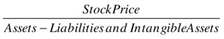
- Notice that only tangible assets, the ones that can be eventually sold, are considered in this equation.
- Price-earnings to growth (PEG): This indicator can be used to compare companies with similar P/E but different growth rates. The formula to calculate this value is simply
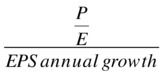
- Earnings before interest, taxes, depreciation, and amortization (EBITDA): This is a measure that can be used to determine how a company is making a profit, and it is based on accounting information provided by the company in every earnings release. The value simply represents how much profit the company made before items such as taxes and related expenses were paid.
- Return on equity (ROE): This ratio is used to determine the percentage of net income generated based on shareholders’ equity. Investors are usually interested in companies able to generate higher income on the same amount of equity. The value is simply calculated as
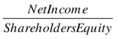
- Forward P/E: This number is similar to the P/E ratio, but instead of being calculated based on existing revenue data, it is a prediction for the next quarter made by analysts. When compared to P/E, this number can be used to determine if analysts expect the revenue to increase, decrease, or stay at the same levels.
Complete Code
Most of the indicators explained in the previous list are easy to calculate, but they are very important when making decisions on which stocks to buy or sell. The class presented in Listing 2-2 offers a good place to store the associated data needed for these indicators, along with the simple calculations needed to produce the desired values with the minimum amount of input.
Listing 2-4 is the complete listing of the FundamentalsCalc class and its associated test code.
Listing 2-4. FundamentalsCalc.h
//
//  FundamentalsCalc.h

#ifndef __FinancialSamples__FundamentalsCalc__
#define __FinancialSamples__FundamentalsCalc__

#include <string>

class FundamentalsCalculator {
public:
    FundamentalsCalculator(const std::string &ticker, double price, double dividend);
    ~FundamentalsCalculator();
    FundamentalsCalculator(const FundamentalsCalculator &);
    FundamentalsCalculator &operator=(const FundamentalsCalculator&);

    void setNumOfShares(int n);
    void setEarnings(double val);
    void setExpectedEarnings(double val);
    void setBookValue(double val);
    void setAssets(double val);
    void setLiabilitiesAndIntangibles(double val);
    void setEpsGrowth(double val);
    void setNetIncome(double val);
    void setShareHoldersEquity(double val);

    double PE();
    double forwardPE();
    double bookValue();
    double priceToBookRatio();
    double priceEarningsToGrowth();
    double returnOnEquity();
    double getDividend();

private:

    std::string m_ticker;
    double m_price;
    double m_dividend;
    double m_earningsEstimate;
    int m_numShares;
    double m_earnings;
    double m_bookValue;
    double m_assets;
    double m_liabilitiesAndIntangibles;
    double m_epsGrowth;
    double m_netIncome;
    double m_shareholdersEquity;
};

#endif /* defined(__FinancialSamples__FundamentalsCalc__) */

//
//  FundamentalsCalc.cpp

#include "FundamentalsCalc.h"

#include <iostream>

FundamentalsCalculator::FundamentalsCalculator(const std::string &ticker,
                                               double price, double dividend) :
m_ticker(ticker),
m_price(price),
m_dividend(dividend),
m_earningsEstimate(0),
m_numShares(0),
m_bookValue(0),
m_assets(0),
m_liabilitiesAndIntangibles(0),
m_epsGrowth(0),
m_netIncome(0),
m_shareholdersEquity(0)
{

}

FundamentalsCalculator::FundamentalsCalculator(const FundamentalsCalculator &v) :
m_ticker(v.m_ticker),
m_price(v.m_price),
m_dividend(v.m_dividend),
m_earningsEstimate(v.m_earningsEstimate),
m_numShares(v.m_numShares),
m_bookValue(v.m_bookValue),
m_assets(v.m_assets),
m_liabilitiesAndIntangibles(v.m_liabilitiesAndIntangibles),
m_epsGrowth(v.m_epsGrowth),
m_netIncome(v.m_netIncome),
m_shareholdersEquity(v.m_shareholdersEquity)
{

}

FundamentalsCalculator::~FundamentalsCalculator()
{

}

FundamentalsCalculator &FundamentalsCalculator::operator=(const FundamentalsCalculator &v)
{
    if (this != &v)
    {
        m_ticker = v.m_ticker;
        m_price = v.m_price;
        m_dividend = v.m_dividend;
        m_earningsEstimate = v.m_earningsEstimate;
        m_numShares = v.m_numShares;
        m_bookValue = v.m_bookValue;
        m_assets = v.m_assets;
        m_liabilitiesAndIntangibles = v.m_liabilitiesAndIntangibles;
        m_epsGrowth = v.m_epsGrowth;
        m_netIncome = v.m_netIncome;
        m_shareholdersEquity = v.m_shareholdersEquity;
    }
    return *this;
}

double FundamentalsCalculator::PE()
{
    return (m_price * m_numShares)/ m_earnings;
}

double FundamentalsCalculator::forwardPE()
{
    return (m_price * m_numShares)/ m_earningsEstimate;
}

double FundamentalsCalculator::returnOnEquity()
{
    return m_netIncome / m_shareholdersEquity;
}

double FundamentalsCalculator::getDividend()
{
    return m_dividend;
}

double FundamentalsCalculator::bookValue()
{
    return m_bookValue;
}

double FundamentalsCalculator::priceToBookRatio()
{
    return (m_price * m_numShares) / (m_assets - m_liabilitiesAndIntangibles);
}

double FundamentalsCalculator::priceEarningsToGrowth()
{
    return PE()/ m_epsGrowth;
}

void FundamentalsCalculator::setNumOfShares(int n)
{
    m_numShares = n;
}

void FundamentalsCalculator::setEarnings(double val)
{
    m_earnings = val;
}

void FundamentalsCalculator::setExpectedEarnings(double val)
{
    m_earningsEstimate = val;
}

void FundamentalsCalculator::setBookValue(double val)
{
    m_bookValue = val;
}

void FundamentalsCalculator::setEpsGrowth(double val)
{
    m_epsGrowth = val;
}

void FundamentalsCalculator::setNetIncome(double val)
{
    m_netIncome = val;
}

void FundamentalsCalculator::setShareHoldersEquity(double val)
{
    m_shareholdersEquity = val;
}

void FundamentalsCalculator::setLiabilitiesAndIntangibles(double val)
{
    m_liabilitiesAndIntangibles = val;
}

void FundamentalsCalculator::setAssets(double val)
{
    m_assets = val;
}

//
//  main.cpp

#include "FundamentalsCalc.h"

#include <iostream>

// the main function receives parameters passed to the program
// and uses class FundamentalsCalculator
int main(int argc, const char * argv[])
{
    FundamentalsCalculator fc("AAPL", 543.99, 12.20);

    // values are in millions
    fc.setAssets(243139);
    fc.setBookValue(165234);
    fc.setEarnings(35885);
    fc.setEpsGrowth(0.22);
    fc.setExpectedEarnings(39435);
    fc.setLiabilitiesAndIntangibles(124642);
    fc.setNetIncome(37235);
    fc.setNumOfShares(891990);
    fc.setShareHoldersEquity(123549);

    std::cout << "P/E: " <<  fc.PE()/1000  << std::endl;  // prices in thousands
    std::cout << "forward P/E: " <<  fc.forwardPE()/1000  << std::endl;
    std::cout << "book value: " <<  fc.bookValue()  << std::endl;
    std::cout << "price to book: " <<  fc.priceToBookRatio()  << std::endl;
    std::cout << "price earnings to growth: " <<  fc.priceEarningsToGrowth()  << std::endl;
    std::cout << "return on equity: " <<  fc.returnOnEquity()  << std::endl;
    std::cout << "dividend: " <<  fc.getDividend()  << std::endl;
    return 0;
}
Running the Code
You can compile the code displayed in Listing 2-4 along with the respective test contained in the main function. The result would be displayed as follows:
$ ./fundamentalind
P/E: 13.5219
forward P/E: 12.3046
book value: 165234
price to book: 4094.9
price earnings to growth: 61463.2
return on equity: 0.301378
dividend: 12.2
Conclusion
In this chapter, I provided an overview of the problems and opportunities in the equities market. As you have seen, being a major part of the financial system, equity trading is an area in which computational problems exist in all phases of analysis and trade execution.
The chapter starts with a short introduction to the equities market, describing the main players and the financial instruments used in the trading process. In the first section you learned how to calculate moving averages using C++. Moving averages are widely used to uncover trends in stock prices. In the same section, I discussed how to calculate the EMA, in which the most recent prices receive a larger weight. The EMA is more responsive to recent changes in price, which may be a better way to make buy or sell decisions in some algorithms.
Next, I presented some code to calculate the volatility of an equity instrument. The notion of volatility is important when making decisions about which instruments to hold in a portfolio. The methods for calculating volatility include using the simple observed range, as well as the probabilistic measure of volatility, also called standard deviation.
In this chapter you have also learned a how to calculate the correlation between two stocks, indicating if there is positive, negative, or no correlation based on their observed prices. Finally, this chapter introduces techniques for modeling and calculating fundamental data about a stock holding. Such a C++ class is easy to create, but it is also very useful when fundamental data is required during the analysis of a particular stock. You can modify this recipe to add new fundamental indicators as needed, and therefore reuse existing code in other areas of your financial applications.
In the next chapter you will learn more about C++ features that are frequently used in the creation of financial software. You will see a number of techniques that are readily available to developers in the financial industry. Such C++ features are able to improve the performance, robustness, and flexibility of most code that is created for the analysis of investments.