![]()
Among other programming techniques for equity markets, Monte Carlo simulation has a special place due to its wide applicability and relatively easy implementation compared to exact, non-stochasatic methods. These algorithms can be used in many applications such as price forecasting and the validation of certain buying strategies, for example.
In this chapter, we provide C++ programming code that can be used either directly or as part of simulation-based algorithms. These examples will introduce some of the most important concepts used in the development of stochastic methods. Following is a quick summary of topics discussed in this chapter:
- Determining definite integrals: random sampling is a powerful way to calculate complicated functions with a minimum of computational effort. You will see how to use stochastic techniques to determine definite integrals.
- Forecasting prices: being a common technique to simulate random price fluctuations, Monte Carlo methods have been frequently used as a way to forecast prices. The ability to repeat the simulation process is a key feature of this method.
- Calculating options prices: among other methods for option pricing forecasting, Monte Carlo techniques have been widely used due to its simplicity. Unlike other mathematical methods, simulations can be quickly coded and generally perform well compared to exact techniques for option price forecasting.
Monte Carlo-Based Integral Computation
Create a class to estimate the integral of a generic function using a Monte Carlo strategy.
Solution
The main concept of Monte Carlo methods is to use a random process to find solutions for a complex problem. While a random solution may not be useful for the problem at hand, it has the important property that it can be repeated with different results. The information that you can gather by looking at a large number of such Monte Carlo results is the secret of such techniques.
A classic example of using Monte Carlo methods is determining the area defined by a curve with random sampling. For example, to find the area of a circle, you can draw several random points and check if they are part of the circle. The area is then determined by the percentage of points inside the circle. As the number of points increase, you will get better approximations for the required area.
An extension of the general idea described previously is the basis for a Monte Carlo strategy for integration. The advantage of using such Monte Carlo methods to integrate functions is that you just need to generate random points in the given range. The simplicity of the strategy makes it possible to estimate the integral of very complicated functions with a minimum of code.
You can see an implementation of this method in the MonteCarloIntegration class. The structure of the class is similar to the examples you saw in Chapter 10, which covers integration. However, the algorithm used involves the generation of random samples, in order to determine the percentage of area under the given function.
To generate uniformly distributed random numbers, we use the uniform_real_distribution class, part of boost::random. This simplifies the generation of samples, avoiding numerical accuracy issues that are common when using other sources of random numbers.
The main part of the implementation can be viewed in the getIntegral member function.
double MonteCarloIntegration::getIntegral(double a, double b)
The code initially determines the maximum and minimum values observed. It uses these numbers to define the total area of sampling. Then, the function generates random numbers and checks if they are inside the curve defined by the function or outside it. At the end, the percentage calculated with this procedure is used to compute the total area of the integral. This process is repeated for the positive and negative parts of the given mathematical function, using the member function integrateRegion. The total value of the integral is then calculated as the positive minus the negative area.
You will find the complete code to integrate a function using the Monte Carlo methods in Listing 14-1. The code is divided into a header and an implementation file. A sample main function is included to show how the class MonteCarloIntegration can be used.
Listing 14-1. Monte Carlo Integration Method
//
// MonteCarloIntegration.h

#ifndef __FinancialSamples__MONTECARLOINTEGRATION_H_
#define __FinancialSamples__MONTECARLOINTEGRATION_H_

template <class T>
class MathFunction;

class MonteCarloIntegration {
public:
        MonteCarloIntegration(MathFunction<double> &f);
        MonteCarloIntegration(const MonteCarloIntegration &p);
        ~MonteCarloIntegration();
        MonteCarloIntegration &operator=(const MonteCarloIntegration &p);

        void setNumSamples(int n);
        double getIntegral(double a, double b);
        double integrateRegion(double a, double b, double min, double max);
private:
    MathFunction<double> &m_f;
    int m_numSamples;

};

#endif /* MONTECARLOINTEGRATION_H_ */

//
// MonteCarloIntegration.cpp

#include "MonteCarloIntegration.h"

#include <cmath>
#include <cstdlib>
#include <iostream>

#include "MathFunction.h"

#include <boost/math/distributions.hpp>

#include <boost/random.hpp>
#include <boost/random/uniform_real.hpp>

static boost::rand48 random_generator;

using std::cout;
using std::endl;

namespace {
        const int DEFAULT_NUM_SAMPLES = 1000;
}

MonteCarloIntegration::MonteCarloIntegration(MathFunction<double>& f)
: m_f(f),
  m_numSamples(DEFAULT_NUM_SAMPLES)
{
}

MonteCarloIntegration::MonteCarloIntegration(const MonteCarloIntegration& p)
: m_f(p.m_f),
  m_numSamples(p.m_numSamples)
{
}

MonteCarloIntegration::~MonteCarloIntegration()
{
}

MonteCarloIntegration& MonteCarloIntegration::operator =(const MonteCarloIntegration& p)
{
        if (this != &p)
        {
                m_f = p.m_f;
                m_numSamples = p.m_numSamples;
        }
        return *this;
}

void MonteCarloIntegration::setNumSamples(int n)
{
        m_numSamples = n;
}

double MonteCarloIntegration::integrateRegion(double a, double b, double min, double max)
{
    boost::random::uniform_real_distribution<> xDistrib(a, b);
    boost::random::uniform_real_distribution<> yDistrib(min, max);

    int pointsIn = 0;
    int pointsOut = 0;
    bool positive = max > 0;

    for (int i = 0; i < m_numSamples; ++i)
    {
        double x = xDistrib(random_generator);
        double y = m_f(x);

        double ry = yDistrib(random_generator);
        if (positive && min <= ry && ry <= y)
        {
            pointsIn++;
        }
        else if (!positive && y <= ry && ry <= max)
        {
            pointsIn++;
        }
        else
        {
            pointsOut++;
        }
    }

    double percentageArea = 0;
    if (pointsIn+pointsOut > 0)
    {
        percentageArea = pointsIn / double(pointsIn + pointsOut);
    }

    if (percentageArea > 0)
    {
        return (b-a) * (max-min) * percentageArea;
    }

    return 0;
}

double MonteCarloIntegration::getIntegral(double a, double b)
{
    boost::random::uniform_real_distribution<> distrib(a, b);

    double max = 0;
    double min = 0;

    for (int i = 0; i < m_numSamples; ++i)
    {
        double x = distrib(random_generator);
        double y = m_f(x);

        if (y > max)
        {
            max = y;
        }
        if (y < min)
        {
            min = y;
        }
    }
    double positiveIntg = max > 0 ? integrateRegion(a, b, 0, max) : 0;
    double negativeIntg = min < 0 ? integrateRegion(a, b, min, 0) : 0;
    return positiveIntg - negativeIntg;
}

// Example function

namespace  {

    class FSin : public MathFunction<double>
    {
    public:
        ~FSin();
        double operator()(double x);
    };

    FSin::~FSin()
    {
    }

    double FSin::operator()(double x)
    {
        return sin(x);
    }

}

int main()
{
        cout << "starting" << endl;
        FSin f;
        MonteCarloIntegration mci(f);
        double integral = mci.getIntegral(0.5, 2.5);
        cout << " the integral of the function is " << integral << endl;

        mci.setNumSamples(20000);
        integral = mci.getIntegral(0.5, 2.5);
        cout << " the integral of the function with 20000 intervals is " << integral << endl;
        return 0;
}
You can compile the files presented in Listing 14-1 using gcc or any other standards-compliant C++ compiler. The result for the sample code in the main function is the following, assuming that you named the executable as monteCarloIntegration:
$ ./monteCarloIntegration
 the integral of the function is 1.74
 the integral of the function with 20000 intervals is 1.6702
Notice that this can change depending on the random source used by the implementation. However, the values should approach the correct value as the number of samples used by the Monte Carlo method increase.
Simulating Asset Prices
Create a C++ class to mimic the price fluctuations of equities in the stock market using a random walk simulation process.
Solution
If there is an area in investment where it is difficult to find closed solutions, that area is financial forecasting. Although there are well-known economic models, any complex system such as the stock market is subject to wild fluctuations that result from so many factors, including wars, natural disasters, and personal choices of important players, among others. Due to the big difficulty of estimating such disparate events, a large part of market forecasting models assume that some form of random process is the source of price fluctuations. In this scenario, Monte Carlo techniques prove to be very useful in the simulation of future market conditions.
In this section, I present a very simple Monte Carlo model that can be used for forecasting purposes. To start the presentation, I introduce a first version of this method using a set of very simple simulation rules. Then, you will see a more complex version of this same principle, using a Gaussian distribution, in the next C++ coding example.
The basic strategy used in price forecasting is to simulate price movements using a “random walk.” A random walk process is a stochastic technique in which the next state of the system is defined only by its previous state (a known price) and the probability distribution for the next possible moves. In the example given in this C++ class, there are three next states, each of them having the same probability. As a result, at each moment in time the price can go up, go down, or stay flat.
To simplify the example of random walk given in this section, we assume that the prices of the underlying asset are moving according to a uniform distribution. In other words, price changes are generated in such a way that the average jump is received as a parameter. Also, the increase or decrease in price is defined using a uniformly distributed random variable, with values determined by the known average.
The code necessary to create this simulation is encapsulated in the RandomWalk class. The class is needed to store the information about parameters for the process: among these parameters is the number of steps (samples) in the Monte Carlo simulation, the initial asset price, and the average step used in the process.
Using these parameters, the getWalk member function runs the simulation and returns a vector of prices generated using this strategy. Figure 14-1 displays a sample result of this random process. Once you store the prices generated by getWalk, your code can perform additional processing, as needed. A common example where this may be useful is during the test of new trading strategies and for determination of their profitability.
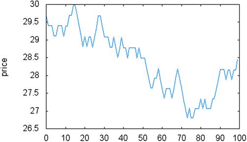
Figure 14-1. Results of the random walk generated by RandomWalk class
The algorithm for random walk used in the RandomWalk class can be tweaked in a number of ways, depending on the demands of your simulation.
- For example, you may want to have the price of the underlying instrument changing more frequently. This can be achieved with the removal of the third branching rule (which allows the price to stay in the same level), and therefore forcing moves either up or down.
- Another variation of the random walk is to have different probabilities for up and high prices —in this way it is possible to simulate a “bull” or “bear” market.
- For a similar purpose as previously, it is possible to change the amount of the price jump (up or down), so that up moves may be bigger than down moves. This would be another way to simulate a directional market, where prices are going up faster than usual.
Listing 14-2 contains the complete code for the RandomWalk class. You will find the implementation in a header file and a cpp file, followed by a sample main function.
Listing 14-2. Implementation for RandomWalk Class
//
// RandonWalk.h

#ifndef __FinancialSamples__RandonWalk__
#define __FinancialSamples__RandonWalk__

#include <vector>

// Simple random walk for price simulation
class RandomWalk {
public:
    RandomWalk(int size, double start, double step);
    RandomWalk(const RandomWalk &p);
    ~RandomWalk();
    RandomWalk &operator=(const RandomWalk &p);

    std::vector<double> getWalk();
private:
    int m_size;     // number of steps
    double m_step;  // size of each step (in percentage)
    double m_start; // starting price
};

#endif /* defined(__FinancialSamples__RandonWalk__) */

//
//  RandonWalk.cpp

#include "RandonWalk.h"

#include <iostream>

using std::vector;
using std::cout;
using std::endl;

RandomWalk::RandomWalk(int size, double start, double step)
: m_size(size),
  m_step(step),
  m_start(start)
{
}

RandomWalk::RandomWalk(const RandomWalk &p)
: m_size(p.m_size),
  m_step(p.m_step),
  m_start(p.m_start)
{
}

RandomWalk::~RandomWalk()
{
}

RandomWalk &RandomWalk::operator=(const RandomWalk &p)
{
    if (this != &p)
    {
        m_size = p.m_size;
        m_step = p.m_step;
        m_start = p.m_start;
    }
    return *this;
}

std::vector<double> RandomWalk::getWalk()
{
    vector<double> walk;
    double prev = m_start;

    for (int i=0; i<m_size; ++i)
    {
        int r = rand() % 3;
        double val = prev;
        if (r == 0) val += (m_step * val);
        else if (r == 1) val -= (m_step * val);
        walk.push_back(val);
        prev = val;
    }
    return walk;
}

int main()
{
    RandomWalk rw(100, 30, 0.01);
    vector<double> walk = rw.getWalk();
    for (int i=0; i<walk.size(); ++i)
    {
        cout << ", " << i << ", " << walk[i];
    }
    cout << endl;
    return 0;
}
To run the code presented in Listing 14-2, first you need to compile it using a standards-compliant compiler such as gcc or Visual Studio. Here are the first few lines of the random walk using the given parameters: initial price of $30, step of 1%, and 100 steps.
./randomWalk
, 0, 29.7, 1, 29.403, 2, 29.403, 3, 29.403, 4, 29.109, 5, 29.109, 6, 29.4001, 7, 29.4001, 8, 29.4001, 9, 29.1061, 10, 29.3971, 11, 29.3971, 12, 29.6911, 13, 29.6911, 14, 29.988, 15, 29.988, 16, 29.6881, 17, 29.3912, 18, 29.0973, 19, 28.8064, 20, 29.0944, 21, 28.8035, 22, 29.0915, 23, 29.0915, 24, 28.8006, 25, 29.0886, 26, 29.3795, 27, 29.6733, 28, 29.6733, 29, 29.3765, 30, 29.0828, 31, 29.0828, 32, 29.0828, 33, 28.792, 34, 28.792, 35, 29.0799, 36, 28.7891, 37, 28.5012, 38, 28.7862, 39, 29.0741, 40, 28.7833, 41, 28.7833, 42, 28.4955, 43, 28.7804, 44, 28.7804, 45, 28.7804, 46, 28.7804, 47, 28.4926, 48, 28.7776, 49, 28.4898, 50, 28.4898, 51, 28.4898, 52, 28.2049, 53, 27.9228, 54, 27.6436, 55, 27.6436, 56, 27.92, 57, 27.92, 58, 28.1992, 59, 27.9173,
Figure 14-1 displays a plot of the random walk generated by one execution of the sample code. Notice how prices start near the $30 mark and display a behavior similar to real variations observed on the stock market.
Calculating Option Probabilities
Implement a C++ solution to compute European options probabilities for events such as finishing above the strike price, finishing below the strike price, or finishing between two given prices.
Solution
Options are a very popular type of equity derivatives, which can be bought in most retail investment accounts. With options, you pay a price for the privilege of buying or selling a stock for a particular price during a limited period of time. Hence the designation “option,” since you have the option, not the obligation, of performing the transaction.
A call option gives the right to buy at a particular price, while a put option gives the right to sell at a particular price. The exercise price is called the strike. Depending on the relationship between the current price of the stock and the strike price, an option can be classified into one of the three categories.
- In the money (ITM): the strike price is lower than the current price of the stock, for call options. For put options, the strike price should be above the current stock price.
- Out of the money (OTM): the strike price is higher than the current price of the stock, for call options. For put options, the strike price should be below the current stock price.
- At the money (ATM): the strike price is close to the current price of the underlying stock.
These different relationships between strike price and stock price determine different probabilities of an option to become profitable, as we will see in the remainder of this section.
To achieve profitability, a call option needs the stock price to rise above the strike price. When this happens, the price for the position is given by the difference between the strike price and the stock price, plus whatever time value the option might still have. For put options this is reversed, and the option becomes profitable when the stock prices decreases in comparison to the strike price.
Another concept in options is the style of exercise (i.e., buying or selling the underlying stock). European-style options allow the exercising of the option only at the end of its target period. American-style options, on the other hand, allow exercising to happen at any moment in time. In this section I consider European options only, since the analysis considers only the price of the stock at the option expiration. It is not hard, however, to extend the techniques explained to handle American-style options.
Figure 14-2 shows the profit profile for an option contract. The data assumes that the contract costs $5, with a strike price of $90. In this case, for any final price of the underlying stock that is below $90, the full loss of the option price is realized. On the other hand, the loss is capped, and the investor will not suffer any losses other than the price of the contract. When the underlying asset price achieves the strike price of $90, the loss of the position starts to decrease, getting to an even point at $95. From that point on, any additional price increase represents additional profit for the option position, and gains are unlimited to the upside.
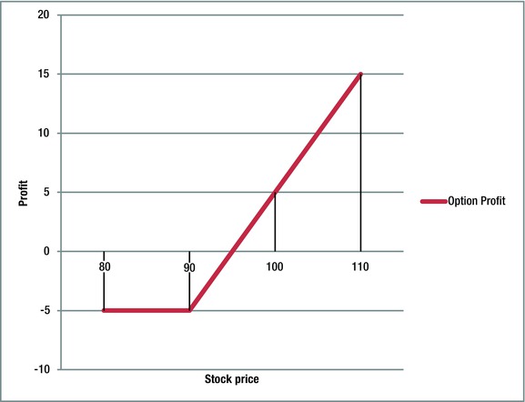
Figure 14-2. Profit potential for an option call contract
Determining Profit Probabilities
In this section you will learn how to use Monte Carlo techniques to determine profit probabilities for equity options. As you have seen previously, all that is necessary to find the profit for a call option is to calculate the price of the underlying asset at expiration and check if the final price is above the strike price. For put options, the process is the same but instead you need to check if the final price is below the strike price.
The first step in creating a Monte Carlo simulation for this problem is to define the parameters of the random process. The pricing of options is defined by what is called the Black-Scholes model, where prices are assumed to be normally distributed. For this reason, you will use a random walk with Gaussian distribution for price changes. At each step only two possibilities are available in this random process: prices either go up or go down with 50% of chance. The price change is then determined by the normal distribution with variance that is given as an input parameter. Figure 14-3 presents an example of Gaussian random walk. Notice how similar this looks to actual price fluctuations, when compared to real data for stocks.
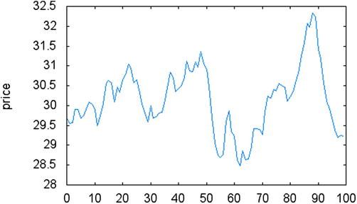
Figure 14-3. Example of price movement created using a Gaussian random walk
Once the random walk is generated, one can start to use the data for forecasting and related price analysis. In this case, you would like to estimate the probabilities of some events, such as finishing above a certain price level. To answer these questions, you just need to use the standard Monte Carlo procedure: repeat the random walk and store the results. After this process is performed several times, it is possible to analyze the distribution of results in which the final price was above a certain target.
For example, suppose you want to answer the question: what is the probability of the price finishing above the strike price? To do this, perform the random walk for a large number of tests, and calculate the percentage of these tests in which the price finished above the strike. The same approach can be used to collect related information, such as the probability of finishing below the strike price, or the probability of finishing between two given prices.
The implementation is given in the OptionsProbabilities class. The important member functions are the following:
double probFinishAboveStrike();
double probFinishBelowStrike();
double probFinalPriceBetweenPrices(double lowPrice, double highPrice);
std::vector<double> getWalk();
The three first member functions calculate the desired probabilities. The last member function, getWalk, returns a vector that stores a sample random walk for further analysis. The OptionsProbabilities class internally uses the getLastPriceOfWalk member function, which returns the last observed price observed in a Gaussian walk. This price is the one stored as input to the probability calculations.
Finally, price changes are computed using the Gaussian distribution. Random values according to this distribution are generated using the gaussianValue member function:
double OptionsProbabilities::gaussianValue(double mean, double sigma)
{
        boost::random::normal_distribution<> distrib(mean, sigma);
        return distrib(random_generator);
}
To see how these functions are used together, consider the implementation of probFinishAboveStrike:
double OptionsProbabilities::probFinishAboveStrike()
{
    int nAbove = 0;
    for (int i=0; i<m_numIterations; ++i)
    {
        double val = getLastPriceOfWalk();
        if (val >= m_strike)
        {
            nAbove++;
        }
    }

    return nAbove/(double)m_numIterations;
}
The algorithm repeats as many iterations as are defined by the member variable m_numIterations. At each iteration, you request a new Gaussian random walk and store the last observed value. If the value satisfies the required property (in this case finishing above the strike price), then it is counted as an occurrence of the event. Finally, the member function returns the empirical probability defined by the percentage of favorable cases.
Listing 14-3 presents the random walk method to evaluate option probabilities. A sample main function is given at the end of the listing, showing how the OptionsProbabilities class can be invoked.
Listing 14-3. Class OptionsProbabilities
//
// OptionsProbabilities.h

#ifndef __FinancialSamples__OptionsProbabilities__
#define __FinancialSamples__OptionsProbabilities__

#include <vector>

class OptionsProbabilities {
public:
    OptionsProbabilities(double initialPrice, double strike, double avgStep, int nDays);
    OptionsProbabilities(const OptionsProbabilities &p);
    ~OptionsProbabilities();
    OptionsProbabilities &operator=(const OptionsProbabilities &p);

    void setNumIterations(int n);

    double probFinishAboveStrike();
    double probFinishBelowStrike();
    double probFinalPriceBetweenPrices(double lowPrice, double highPrice);
    std::vector<double> getWalk();
private:
    double m_initialPrice;
    double m_strike;
    double m_avgStep;
    int m_numDays;
    int m_numIterations;

    double gaussianValue(double mean, double sigma);
    double getLastPriceOfWalk();
};

#endif /* defined(__FinancialSamples__OptionsProbabilities__) */

//
// OptionsProbabilities.cpp

#include "OptionsProbabilities.h"

#include <boost/random/normal_distribution.hpp>
#include <boost/random.hpp>

using std::vector;
using std::cout;
using std::endl;

static boost::rand48 random_generator;

namespace  {
    const int NUM_ITERATIONS = 1000;
}

OptionsProbabilities::OptionsProbabilities(double initialPrice,
                                           double strike, double avgStep, int nDays)
: m_initialPrice(initialPrice),
  m_strike(strike),
  m_avgStep(avgStep),
  m_numDays(nDays),
  m_numIterations(NUM_ITERATIONS)
{
}

OptionsProbabilities::OptionsProbabilities(const OptionsProbabilities &p)
: m_initialPrice(p.m_initialPrice),
  m_strike(p.m_strike),
  m_avgStep(p.m_avgStep),
  m_numDays(p.m_numDays),
  m_numIterations(p.m_numIterations)
{
}

OptionsProbabilities::~OptionsProbabilities()
{
}

OptionsProbabilities &OptionsProbabilities::operator=(const OptionsProbabilities &p)
{
    if (this != &p)
    {
        m_initialPrice = p.m_initialPrice;
        m_strike = p.m_strike;
        m_avgStep = p.m_avgStep;
        m_numDays = p.m_numDays;
        m_numIterations = p.m_numIterations;
    }
    return *this;
}

void OptionsProbabilities::setNumIterations(int n)
{
    m_numIterations = n;
}

double OptionsProbabilities::probFinishAboveStrike()
{
    int nAbove = 0;
    for (int i=0; i<m_numIterations; ++i)
    {
        double val = getLastPriceOfWalk();
        if (val >= m_strike)
        {
            nAbove++;
        }
    }

    return nAbove/(double)m_numIterations;
}

double OptionsProbabilities::probFinishBelowStrike()
{
    int nBelow = 0;
    for (int i=0; i<m_numIterations; ++i)
    {
        double val = getLastPriceOfWalk();
        if (val <= m_strike)
        {
            nBellow++;
        }
    }

    return nBelow/(double)m_numIterations;
}

double OptionsProbabilities::probFinalPriceBetweenPrices(double lowPrice, double highPrice)
{
    int nBetween = 0;
    for (int i=0; i<m_numIterations; ++i)
    {
        double val = getLastPriceOfWalk();
        if (lowPrice <= val && val <= highPrice)
        {
            nBetween++;
        }
    }

    return nBetween/(double)m_numIterations;
}

double OptionsProbabilities::gaussianValue(double mean, double sigma)
{
        boost::random::normal_distribution<> distrib(mean, sigma);
        return distrib(random_generator);
}

double OptionsProbabilities::getLastPriceOfWalk()
{
    double prev = m_initialPrice;

    for (int i=0; i<m_numDays; ++i)
    {
        double stepSize = gaussianValue(0, m_avgStep);
        int r = rand() % 2;
        double val = prev;
        if (r == 0) val += (stepSize * val);
        else val -= (stepSize * val);
        prev = val;
    }
    return prev;
}

std::vector<double> OptionsProbabilities::getWalk()
{
    vector<double> walk;
    double prev = m_initialPrice;

    for (int i=0; i<m_numDays; ++i)
    {
        double stepSize = gaussianValue(0, m_avgStep);
        int r = rand() % 2;
        double val = prev;
        if (r == 0) val += (stepSize * val);
        else val -= (stepSize * val);
        walk.push_back(val);
        prev = val;
    }
    return walk;
}

int main()
{
    OptionsProbabilities optP(30, 35, 0.01, 100);

    cout << " above strike prob: " << optP.probFinishAboveStrike() << endl;
    cout << " below strike prob: " << optP.probFinishBelowStrike() << endl;
    cout << " between 28 and 32  prob: " << optP.probFinalPriceBetweenPrices(28, 32) << endl;

    return 0;
}
To run the code in Listing 14-3, you can use any standards-compliant C++ compiler such as gcc, llvm, or Visual C++. Once you compile the code and generate an executable file, the application can be run with the following results (exact numbers can vary depending on the random numbers used):
above strike prob: 0.055
below strike prob: 0.946
between 28 and 32 prob: 0.512
As you can see, the application is able to determine with good precision the probability that the price will finish above or below the strike. This is confirmed by the fact that the two first values add up to close to 100%. The approximation can still be improved by increasing the number of simulated random walks.
Conclusion
Monte Carlo methods are a general approach to problem solving that use randomization as a way to compute solutions that would be otherwise very difficult to find exactly. Due to the inherent randomness of financial markets, Monte Carlo methods appear as an important tool in the hands of the financial engineer and software developer.
You have seen in this chapter that such simulation techniques can be used to find quick solutions to diverse problems in the area of finance. For example, a common way to use Monte Carlo simulations is to forecast possible economic scenarios dictated by price variations. While this is a difficult task for traditional mathematical methods, one can easily design efficient algorithms such as a random walk. Such algorithms offer the ability to forecast prices using just a few input parameters based on past behavior.
In the first coding example, in Listing 14-1, we used a Monte Carlo technique to calculate the definite integral of a general function. While there are efficient ways to solve this problem with deterministic numeric algorithms, this problem shows the basic features of Monte Carlo methods and how their results can be interpreted and improved.
In Listing 14-2, you saw how to create a very simple random walk, which is one of the basic tools available for price simulation using Monte Carlo methods. You saw how to implement a version of random walk where price changes are uniformly distributed. You also saw a few common variations of the standard method, which are frequently used in applications.
Next, you learned about the use of Monte Carlo methods to calculate profit probabilities for options. The C++ class in Listing 14-3 illustrated a scheme that is easy to implement and can be used to analyze options and their possible profit scenarios. You have seen that using simulation and a few assumptions about price changes one can easily determine the probability that a given stock will be in a certain price range within a number of days.
This chapter completes the discussion of the major mathematical tools used in financial software. In the next chapter you will start to explore additional programming technologies that can be employed to support the creation and maintenance of such financial applications. You will see a number of examples that show how to integrate existing C++ code with other popular scripting languages, such as Python and Lua.