![]()
Solving ODEs and PDEs
The solution of ODEs (ordinary differential equations) and PDEs (partial differential equations) is at the heart of many techniques used in the analysis of financial markets. Important analytical tools for derivative valuation such as the Black-Scholes model for stock options and other derivatives can be directly represented as differential equations. Such equations need to be regularly solved in order to determine the price of financial instruments traded in the global markets. This creates the need for high-performance code, capable of finding efficient solutions to these mathematical models.
Due to the large number of applications of ODEs and PDEs in science, engineering, and finance, several methods to solve them have been developed. In addition to the exact mathematical methods, capable of analyzing and finding the solution to differential equations, a software engineer also has to deal with purely computational approaches, as well as their implementation in C++. Since the application of differential equations to financial problems is such a large area, in this chapter I am able to present only an overview of the methods most frequently used for their solution.
The programming examples discussed in this chapter cover a few particular aspects of ODE and PDE modeling and applications. Topics that you will explore include the following:
- Euler’s method for ODEs: an algorithm that is simple to implement and can be applied directly to any first-order ODE.
- Runge-Kutta method: an improvement over the general ideas of Euler’s algorithm, the Runge-Kutta method provides better stability and accuracy for the solution to ODEs.
- Black-Scholes equation: a general discussion of the Black-Scholes PDE and an overview of the forward method to solve this model.
Solving Ordinary Differential Equations
Create a class to solve ODEs using Euler’s method.
I start the discussion of differential equations with some methods for the numerical solution to ordinary differential equations. Before I can start with a first example, however, let’s remember some of the relevant facts about ODEs.
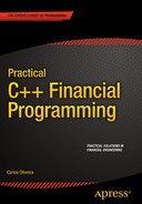
An ordinary differential equation is an equation that includes the rate of change (derivative) with respect to a single variable in one or more of its terms. Given a differential equation, its order is defined as the maximum order of any of the derivatives included in the equation. Following are a few examples of ODEs:
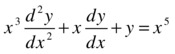
Both equations involve the derivative of the variable y with respect to x. In the first equation, the derivative is applied twice, resulting in the term d2y/dx2, which means that it is a second-order ODE. The second equation contains only a first-order derivative with respect to x, making it a first-order ODE.
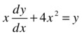
Standard equations (the ones that don’t involve derivatives) usually have solutions that can be expressed as a single number. ODEs, however, include derivatives and therefore their solutions are better described as being one or more functions, which together satisfy the conditions implied by the derivatives. For example, the following well-known differential equation describes Newton’s law of gravity:
The solution of such an equation is a general function describing the velocity and acceleration of an object. To find out a numeric solution to such a particular problem, you would need to supply one or more initial conditions that, when plugged into the general solutions, will provide an explicit value for x in the given equation.
As you have seen from the previous example, numerically solving an ODE involves working with initial conditions that can be substituted in the general function that solves the equation. As a consequence, numerical methods to solve ODEs (and PDEs) require the determination of initial conditions as a prerequisite to find their numerical solutions.
There are two main types of methods that can be used to solve differential equations. The first kind of solution is based on symbolic methods. Such methods use algebraic techniques, including the known rules of differentiation and integration, to simplify and derive a closed solution to a differential equation. Symbolic methods can be performed manually or by computers, and there is a class of software that was created specifically to perform such symbolic manipulations. Main examples include Mathematica, Maple, and Maxima, among others.
While symbolic methods are very useful in solving certain classes of ODEs and PDEs, many differential equations are too complex to be solved to a closed form using symbolic manipulation. Moreover, such symbolic techniques are very specialized and are normally used only during the modeling and exploration phases, when the engineer or mathematician is creating a model based on differential equations. For these reasons, symbolic techniques are mostly confined to specialized software packages, rather than being used as libraries for general-purpose languages.
The second class of techniques for solving differential equations is based on numerical algorithms. These algorithms are more general in the sense that they can be applied to any differential equation, as long as some basic requirements are met. Moreover, many common differential equations have no known closed solutions, and in such cases numerical methods are the only ones available. Because numerical methods for ODEs and PDEs can be implemented using standard programming techniques, they are commonly used as part of mathematical libraries for programming languages such as FORTRAN and C++.
The first numerical algorithm for ODEs you will learn about is a simple technique called Euler’s method, which is based on the successive evaluation of the desired ODE at predetermined steps. Starting from a given initial condition, Euler’s method tries to find the next value of the differential equation, using approximation formulas that are applied at predetermined intervals.
The idea of Euler’s method is to correct possible errors in the evaluation of the ODE when starting from the given initial condition. For example, suppose that you want to evaluate an ODE at desired point c, when starting from initial condition x0. To make the argument simpler, assume that x0 ≤ c, although the same ideas are valid in the other direction. To solve the ODE, the idea of this algorithm is to perform the evaluation in N steps, where N is a given parameter. As a consequence, the step size is given by

Let’s assume that the differential equation can be represented as a first-order ODE in the following general form:
![]()
Also, the initial condition (x0,y0) is known.
In general terms, at each step (given by the value h) Euler’s algorithm will try to determine the correct value of the solution for the ODE for that small step size. The biggest problem, however, is that the solution to the differential equation is not known in an explicit way, so the algorithm has to guess a particular value for each step. Since the step size is a small interval, a possible way to guess the value of the function is to approximate it using a straight line. If we call yt the value of the function at step t, then this leads to the following approximation for yt:
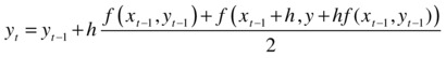
In other words, the algorithm takes the mean value of the linear approximation between the previous point and the next point, as the next approximation to the small value between yt–1 and yt.
Euler’s algorithm is a simple example of what is known as a predictor-corrector algorithm. Such methods work by predicting where a function might be in the subsequent iteration, which in this case is performed using a linear approximation. The next step is to correct this prediction, in this case by taking the average value. The same strategy is repeated in many other algorithms, although with more complex approximation schemes.
One of the biggest issues when using Euler’s algorithm is controlling for errors in the result. As you have seen, the step size for Euler’s method is one of the input parameters for its implementation and indicates the frequency with which we want to update the results of the differential equation. The finer grained the steps we take in this evaluation process, the closer to the real function we get. On the other hand, two problems occur when we increase the number of steps in the ODE evaluation. First, there is the increase in running time due to the additional calculations that become necessary. Second, and of even more concern, is the fact that by increasing the number of steps you might be increasing the numeric errors that are inevitable when doing calculations on a computer. Solving these precision problems leads to the development of other methods, as you see in the next section.
Complete Code
Euler’s method, as described in the previous section, is implemented in the EulersMethod class displayed in Listing 11-1. The important method in this class is solve(), which receives as parameters the number of steps, the initial values x0 and y0, and the target point c.
Listing 11-1. Implementation for Euler’s Method for Solving ODEs
//
//  EulersMethod.h

#ifndef __FinancialSamples__EulersMethod__
#define __FinancialSamples__EulersMethod__

template <class T>
class MathFunction;

class EulersMethod {
public:
    EulersMethod(MathFunction<double> &f);
    EulersMethod(const EulersMethod &p);
    ~EulersMethod();
    EulersMethod &operator=(const EulersMethod &p);

    double solve(int n, double x0, double y0, double c);
private:
    MathFunction<double> &m_f;
};

#endif /* defined(__FinancialSamples__EulersMethod__) */

//
//  EulersMethod.cpp

#include "EulersMethod.h"

#include "MathFunction.h"

#include <iostream>

using std::cout;
using std::endl;

EulersMethod::EulersMethod(MathFunction<double> &f)
: m_f(f)
{
}

EulersMethod::EulersMethod(const EulersMethod &p)
: m_f(p.m_f)
{
}

EulersMethod::~EulersMethod()
{
}

EulersMethod &EulersMethod::operator=(const EulersMethod &p)
{
    if (this != &p)
    {
        m_f = p.m_f;
    }
    return *this;
}

double EulersMethod::solve(int n, double x0, double y0, double c)
{
    // problem :   y' = f(x,y) ;  y(x0) = y0

    auto x = x0;
    auto y = y0;
    auto h = (c - x0)/n;

    cout << " h is " << h << endl;

    for (int i=0; i<n; ++i)
    {
        double F = m_f(x, y);
        auto G = m_f(x + h, y + h*F);

        cout << " F: " << F << " G: " << G << endl;

        // update values of x, y
        x += h;
        y += h * (F + G)/2;
        cout << " x: " << x << " y: " << y << endl;

    }

    return y;
}

/// -----

class EulerMethSampleFunc : public MathFunction<double> {
public:
    double operator()(double x) { return x; } // not used
    double operator()(double x, double y);
};

double EulerMethSampleFunc::operator()(double x, double y)
{
    return  3 * x + 2 * y + 1;
}

int main()
{
    EulerMethSampleFunc f;
    EulersMethod m(f);
    double res = m.solve (100, 0, 0.25, 2);
    cout << " result is " << res << endl;
    return 0;
}
Running the Code
You can generate a binary executable from the source code in Listing 11-1 using any standards-compliant compiler such as gcc. Then, you can execute the code to get sample results such as the following for the sample equation f(x) = 3x + 2y + 1:
./eulersMethod
h is 0.02
 F: 1.5     G: 1.62    x: 0.02 y: 0.2812
 F: 1.6224  G: 1.7473  x: 0.04 y: 0.314897
 F: 1.74979 G: 1.87979 x: 0.06 y: 0.351193
 F: 1.88239 G: 2.01768 x: 0.08 y: 0.390193
 // ...
 F: 137.938 G: 143.515 x: 1.94 y: 68.4034
 F: 143.627 G: 149.432 x: 1.96 y: 71.334
 F: 149.548 G: 155.59  x: 1.98 y: 74.3854
 F: 155.711 G: 161.999 x: 2    y: 77.5625
result is 77.5625
Notice that the solution tests the approximation for two cases: when the number of intervals is 100 (the default) and when necessary.
Runge-Kutta Method for Solving ODEs
Implement the Runge-Kutta method for solving ODEs.
In the last section you saw how to use Euler’s method to solve ODEs, a technique that iterates through a series of steps while computing an approximation to the desired differential equations. A problem with Euler’s method, however, is its slow convergence. Due to the first-order approximation used, the method requires a large number of steps if any accuracy is desired. On the other hand, it is also difficult to avoid error propagation when the number of steps increases, which makes it difficult to improve the accuracy of this method.
To reduce some of the problems inherent in Euler’s method, other strategies have been devised. The way these methods work is to use better approximations for each step of the algorithm, so that it is possible to use fewer steps overall to find the desired solution. Also, the improved approximation makes it possible to reduce errors incurred in a single step. One of the most popular of such improved algorithms for the solution of ODEs is called the Runge-Kutta method. Compared to Euler’s method, the Runge-Kutta method uses a different approximation scheme for each new step of the algorithm, which guarantees higher accuracy. As a consequence, you will also have faster convergence when using the Runge-Kutta method.
As before, assume that we are given a first-order differential equation with relation to the x variable:
![]()
The initial condition (x0,y0) is known, and the goal is to calculate the value of the differential equation at some point c. If we define as N the number of steps, the step size can be given as

The Taylor method from calculus can be used to compute the approximation to a function given its derivatives. The approximation found when using the second-order Taylor approximation will give a more accurate result than the linear approximation used in Euler’s algorithm. The formulas used in the original Runge-Kutta algorithm are the following:
![]()
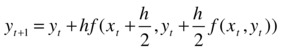
If you employ higher-order approximations derived using the Taylor method you can get even more precise results. The most common of such approximations is the fourth-order Runge-Kutta method. In this case, the formula for yt+1 is given by
![]()
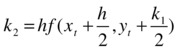
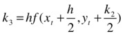
![]()

This method offers good results in terms of fast approximation and is appropriate to solve most ODE problems. The implementation is relatively straightforward, as showed in the code that follows.
Listing 11-2 presents the Runge-Kutta method for solving ODEs. The code organization is similar to what I used for Euler’s method. The main difference resides in the way the next step is defined, which uses the equations based on the Taylor method as explained previously.
Listing 11-2. Implementation of the Runge-Kutta Method to Solve ODEs
//
//  RungeKuttaODEMethod.h

#ifndef __FinancialSamples__RungeKuttaODEMethod__
#define __FinancialSamples__RungeKuttaODEMethod__

template <class T>
class MathFunction;

class RungeKuttaODEMethod {
public:
    RungeKuttaODEMethod(MathFunction<double> &f);
    RungeKuttaODEMethod(const RungeKuttaODEMethod &p);
    ~RungeKuttaODEMethod();
    RungeKuttaODEMethod &operator=(const RungeKuttaODEMethod &p);
    double solve(int n, double x0, double y0, double c);
private:
    MathFunction<double> &m_f;
};

#endif /* defined(__FinancialSamples__RungeKuttaODEMethod__) */

//
//  RungeKuttaODEMethod.cpp

#include "RungeKuttaODEMethod.h"

#include "MathFunction.h"

#include <iostream>

using std::cout;
using std::endl;

RungeKuttaODEMethod::RungeKuttaODEMethod(MathFunction<double> &f)
: m_f(f)
{
}

RungeKuttaODEMethod::RungeKuttaODEMethod(const RungeKuttaODEMethod &p)
: m_f(p.m_f)
{
}

RungeKuttaODEMethod::~RungeKuttaODEMethod()
{
}

RungeKuttaODEMethod &RungeKuttaODEMethod::operator=(const RungeKuttaODEMethod &p)
{
    if (this != &p)
    {
        m_f = p.m_f;
    }
    return *this;
}

double RungeKuttaODEMethod::solve(int n, double x0, double y0, double c)
{
    auto x = x0;
    auto y = y0;
    auto h = (c - x0)/n;

    for (int i=0; i<n; ++i)
    {
        auto k1 = h * m_f(x, y);
        auto k2 = h * m_f(x + (h/2), y + (k1/2));
        auto k3 = h * m_f(x + (h/2), y + (k2/2));
        auto k4 = h * m_f(x + h, y + k3);

        x += h;
        y += ( k1 + 2*k2 + 2*k3 + k4)/6;
    }
    return y;
}

/// -----

class RKMethSampleFunc : public MathFunction<double> {
public:
    double operator()(double x) { return x; } // not used
    double operator()(double x, double y);
};

double RKMethSampleFunc::operator()(double x, double y)
{
    return  3 * x + 2 * y + 1;
}

int main()
{
    RKMethSampleFunc f;
    RungeKuttaODEMethod m(f);
    double res = m.solve (100, 0, 0.25, 2);
    cout << " result is " << res << endl;
    return 0;
}
Running the Code
The code in Listing 11-2 was compiled and tested using gcc. It should work, however, using any standards-compliant compiler. The test code is in the main function, which runs the algorithm using the differential equation y’ = 3x + 2y + 1. The results can be compared with what was achieved with Euler’s method discussed previously.
./rungeKutta
 x: 0.02 y: 0.281216
 x: 0.04 y: 0.314931
 x: 0.06 y: 0.351245
 x: 0.08 y: 0.390266
 // ...
 x: 1.9  y: 62.9518
 x: 1.92 y: 65.6582
 x: 1.94 y: 68.4763
 x: 1.96 y: 71.4107
 x: 1.98 y: 74.466
 x: 2    y: 77.6472
result is 77.6472
The sample output shows the convergence of the algorithm, with 100 iterations. You can see the complete results displayed in Figure 11-1.
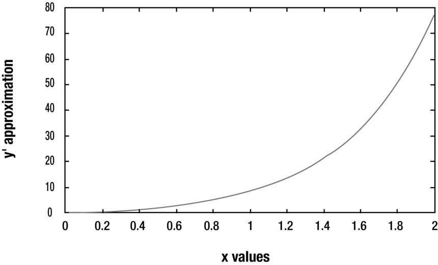
Figure 11-1. Successive steps of the Runge-Kutta algorithm for the previous example, with N=100
Solving the Black-Scholes Equation
Create a C++ class to solve the Black-Scholes equation using the forward method.
The Black-Scholes equation is one of the best known methods to price derivatives. It was developed in the 1970s to provide a better model of European-style options, but since then the basic model has been extended and tested on multiple derivatives markets. While the original assumptions of the Black-Scholes equation are not exactly respected in the real markets, the model works as an excellent analytical tool to price instruments that present volatile behavior as observed in the stock market.
Remember that an option is a contract that allows the holder to buy (or sell) a stock at a particular price in a given time in the future. For example, a call option on MSFT at $30 for July of the next year gives its owner the right (but not the duty) to buy MSFT for the price of $30 in July, irrespective of the real price at that date. Therefore, if MSFT stock price is significantly higher than $30 this operation will result in a profit. At $30 or lower prices, however, this option will result in a loss. Similarly, you can do the same analysis for a put, which is the right to sell a stock at the given price in the future. A call produces higher profits when the price for the underlying rises, with a fixed maximum loss. On the other hand, a put produces higher profits when prices for the underlying asset decrease, also with a fixed maximum loss.
The Black-Scholes model defines what should be the present value of a call option (a similar analysis works for put options). It considers the following input values:
- S: the price of the underlying instrument.
- K: the strike price for the option.
- T: the remaining time for the option contract.
- V: the current volatility of the underlying asset.
- r: the current interest rate on deposits.
Using this information, the Black-Scholes model concludes that the relationship between the current price of the option and the input variables is given by a PDE, as follows:
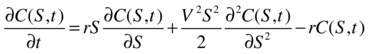
Here, the implicit function C(S,t) is the price or the derivative, which depends on the underlying price S, and the time t.
There are several ways to solve differential equations like the previous one. The one you will use in this section is called the forward method. The general idea of solving PDEs is not very different from what you have seen for ODEs: take small steps toward the desired point that needs to be calculated, and evaluate the differential equation at these intermediate points using some kind of approximation. Unlike ODEs, which have only one dimension, however, PDEs have partial derivatives over two or more variables. In this case, we have partial derivatives in relation to the variables t and S. When this happens, the approximations become more complicated, because one needs to determine the shape of the small intervals at which the PDE will be evaluated. For example, the simplest scheme would be to divide the two-dimensional space into small rectangles and approximate over these small elements. Depending on the class of PDE, one can come up with more complicated and more precise ways to divide the domain and approximate the true value of the partial equation.
The forward difference method is an extension of Euler’s method for PDEs. For the two-dimensional case, it can be used to divide the domain into rectangular elements. For this method to work, you can assume that the stock price domain (S) varies between 0 and MaxS, a constant number that is in practice much higher than the desired strike price. The time domain varies from 0 (current date) to the future time (T) in which the option contract expires. Using these assumptions, the next task is to derive the equations that approximate the PDE at the next step, which can be done again using the Taylor method discussed earlier.
The initial conditions for the forward method are derived from the gain-loss equation at expiration. At that time, the value of an option is the positive difference between the stock price and the strike price, that is, max(S–K,0). Therefore, the steps of the algorithm are inverted in the time dimension, starting from timeT and moving backward to the present.
The resulting algorithm is presented in member function solve of class BlackScholesForwardMethod. The initial part of the function calculates terms of the equation that are unchanged over time. The three main factors are stored in the vectors a, b, and c.
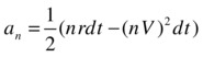
![]()
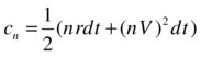
The next step is to initialize the process using the given initial conditions. The calculated prices are stored in the two-dimensional vector u, which is initialized using the prices at expiration time. Then, the algorithm proceeds to compute the values for each of the time periods starting from expiration. At each day, starting from the day before expiration, the price of the option is calculated for each small increase in the underlying price. The option price for underlying value S depends on the price of the next day for values S – dS, S, and S + dS, where dS is a small increase in price, as determined by the parameter nx. Therefore, we have
![]()
Complete Code
Listing 11-3 displays the complete implementation for the Black-Scholes forward method. You will find the code in class BlackScholesForwardMethod, along with a sample of its use in function main().
Listing 11-3. Black-Scholes Forward Method Implementation
//
//  BlackScholesForwardMethod.h

#ifndef __FinancialSamples__BlackScholesForwardMethod__
#define __FinancialSamples__BlackScholesForwardMethod__

#include <vector>

class BlackScholesForwardMethod {
public:
    BlackScholesForwardMethod(double expiration, double maxPrice, double strike, double intRate);
    BlackScholesForwardMethod(const BlackScholesForwardMethod &p);
    ~BlackScholesForwardMethod();
    BlackScholesForwardMethod &operator=(const BlackScholesForwardMethod &p);

    std::vector<double> solve(double volatility, int nx, int timeSteps);
private:
    double m_expiration;
    double m_maxPrice;
    double m_strike;
    double m_intRate;
};

#endif /* defined(__FinancialSamples__BlackScholesForwardMethod__) */

//
//  BlackScholesForwardMethod.cpp

#include "BlackScholesForwardMethod.h"

#include <cmath>
#include <algorithm>
#include <vector>
#include <iostream>
#include <iomanip>

using std::vector;
using std::cout;
using std::endl;
using std::setw;

BlackScholesForwardMethod::BlackScholesForwardMethod(double expiration, double maxPrice,
                                                     double strike, double intRate)
: m_expiration(expiration),
  m_maxPrice(maxPrice),
  m_strike(strike),
  m_intRate(intRate)
{
}

BlackScholesForwardMethod::BlackScholesForwardMethod(const BlackScholesForwardMethod &p)
: m_expiration(p.m_expiration),
  m_maxPrice(p.m_maxPrice),
  m_strike(p.m_strike),
  m_intRate(p.m_intRate)
{
}

BlackScholesForwardMethod::~BlackScholesForwardMethod()
{
}

BlackScholesForwardMethod &BlackScholesForwardMethod::operator=(const BlackScholesForwardMethod &p)
{
    if (this != &p)
    {
        m_expiration = p.m_expiration;
        m_maxPrice = p.m_maxPrice;
        m_strike = p.m_strike;
        m_intRate = p.m_intRate;
    }
    return *this;
}

vector<double> BlackScholesForwardMethod::solve(double volatility, int nx, int timeSteps)
{
    double dt = m_expiration /(double)timeSteps;
    double dx = m_maxPrice /(double)nx;

    vector<double> a(nx-1);
    vector<double> b(nx-1);
    vector<double> c(nx-1);

    int i;
    for (i = 0; i < nx - 1; i++)
    {
        b[i] = 1.0 - m_intRate * dt - dt * pow(volatility * (i+1), 2);
    }

    for (i = 0; i < nx - 2; i++)
    {
        c[i] = 0.5 * dt * pow(volatility * (i+1), 2) + 0.5 * dt * m_intRate * (i+1);
    }

    for (i = 1; i < nx - 1; i++)
    {
        a[i] = 0.5 * dt * pow(volatility * (i+1), 2) - 0.5 * dt * m_intRate * (i+1);
    }

    vector<double> u((nx-1)*(timeSteps+1));

    double u0 = 0.0;
    for (i = 0; i < nx - 1; i++)
    {
        u0 += dx;
        u[i+0*(nx-1)] = std::max(u0 - m_strike, 0.0);
    }

    for (int j = 0; j < timeSteps; j++)
    {
        double t = (double)(j) * m_expiration /(double)timeSteps;

        double p = 0.5 * dt * (nx - 1) * (volatility*volatility * (nx-1) + m_intRate)
        * (m_maxPrice-m_strike * exp(-m_intRate*t ) );

        for (i = 0; i < nx - 1; i++)
        {
            u[i+(j+1)*(nx-1)] = b[i] * u[i+j*(nx-1)];
        }
        for (i = 0; i < nx - 2; i++)
        {
            u[i+(j+1)*(nx-1)] += c[i] * u[i+1+j*(nx-1)];
        }
        for (i = 1; i < nx - 1; i++)
        {
            u[i+(j+1)*(nx-1)] += a[i] * u[i-1+j*(nx-1)];
        }
        u[nx-2+(j+1)*(nx-1)] += p;
    }

    return u;
}

int main()
{
    auto strike = 5.0;
    auto intRate = 0.03;
    auto sigma = 0.50;
    auto t1 = 1.0;
    auto numSteps = 11;
    auto numDays = 29;
    auto maxPrice = 10.0;

    BlackScholesForwardMethod bsfm(t1, maxPrice, strike, intRate);
    vector<double> u = bsfm.solve(sigma, numSteps, numDays);

    double minPrice = .0;
    for (int  i=0; i < numSteps-1; i++)
    {
        double s = ((numSteps-i-2) * minPrice+(i+1)*maxPrice)/ (double)(numSteps-1);
        cout << "  " << s << "  " << u[i+numDays*(numSteps-1)] << endl;
    }
    return 0;
}
Running the Code
To test the code displayed in Listing 11-3 you can build it using any standards-compliant compiler. I run this code using the llvm C++ compiler, with the following results:
./blackScholes
  1  0.000452875
  2  0.0148578
  3  0.109172
  4  0.361706
  5  0.784941
  6  1.34918
  7  2.016
  8  2.75175
  9  3.53055
 10  4.33362
This result means, for example, that 29 days from expiration, a call option with strike price $5 and volatility 0.5 would be valued at $1.3 when the price of the underlying is $6. Notice that you can use this code to calculate prices for each price level ranging from $1 up to $10. You can also modify the code to compute option prices for more expensive stocks.
Conclusion
Solving differential equations is a big part of financial analysis techniques. Such techniques are used in many areas where the price of assets is determined by complex differential equations such as the Black-Scholes model, which is the main technique used by banks to price equity derivatives and related investments.
In this chapter I introduced you to the topic of numerical solutions of differential equations. Although this is a large area that cannot be easily covered in a single chapter, it is useful to understand the basic techniques and how they are employed in the field of financial programming.
Euler’s method for ODEs is the first method discussed. Its main idea is to perform several steps, where each step approximates the result of the differential equation. The second method, the Runge-Kutta algorithm, is an improvement on this general strategy, using higher-order Taylor approximations that make the algorithm more accurate and avoid some of the weaknesses of Euler’s method. You have seen how to implement both algorithms in C++, with test data that demonstrates their convergence.
The Black-Scholes equation is one of the most important mathematical models in modern finance. While there are several robust and efficient algorithms for its solution, I present a simple method based on forward differences. You have seen how the general solution strategy works, and how it can be efficiently implemented in C++.
Finding solutions to equations that model market behavior as viewed in this chapter is generally the beginning of a process of data analysis. Another step is to find the best solution that meets a particular investment goal. For this purpose, a number of optimization techniques have been developed. In the next chapter, I present some general optimization methods that have been successfully used in the analysis of financial investments, along with their implementation in C++.