
CHAPTER 5 Dealing with Faults
Learning objectives of this chapter are to understand:
• The concepts and roles of fault avoidance, fault elimination, fault tolerance, and fault forecasting.
• How to avoid the introduction of faults into a system.
• What can be done to eliminate the faults in a system.
• What can be done to tolerate the faults that remain in a system during operation.
• What can be done to forecast the effects of the faults that remain in a system during operation.
5.1 Faults and Their Treatment
Once we have done the best we can to determine the faults to which a system might be subject, we have to do something about what we found. Recall that there are four approaches to dealing with faults: avoidance, elimination, tolerance, and forecasting. As shown in Figure 5.1, with avoidance we are trying to stop faults from entering the system during development, with elimination we are trying to remove those that manage to enter the system during development, with tolerance we are trying to keep the system operating despite the presence of faults, and with forecasting we are trying to assess the effects of faults that remain in a system and will not be tolerated. In any system under development, each fault that is identified by means such as fault tree analysis has to be dealt with by one of these means.
The preference is always to use the four approaches in the order listed above. We must start by trying to avoid faults. Only if we cannot avoid them should we try to eliminate them. Only if we cannot eliminate them should we try to tolerate them. And finally, if we cannot tolerate them, then we have to resort to trying to forecast them.
Software faults are our biggest concern, and so we will focus on them. This concern means, of course, that we will focus on design faults. Despite this focus, as software engineers we have to be familiar with degradation faults, and so we will discuss them as necessary. In addition, we need to be familiar with Byzantine faults, and they are discussed at the end of this chapter in Section 5.7.
5.2 Fault Avoidance
Fault avoidance means building a system in which a particular fault or class of faults does not arise. This idea is powerful but somewhat counter-intuitive. If we could avoid all faults, we could be confident that our system would meet its dependability goals. Even if we could avoid only some faults, our task would be simplified, and we could focus our attention on those faults that could not be avoided. But how can we actually avoid faults?
5.2.1 Degradation Faults
For degradation faults, fault avoidance is not possible in an absolute sense. In the end, essentially any device built with any technology has a non-zero probability of failure per unit time. In other words, if you wait long enough, any device will fail.
In some cases, however, we can proceed as if degradation faults have been avoided, provided the rate of manifestation of the fault is known to be sufficiently small. This idea is especially important if the dependability requirements for a system do not require long periods of operation. If reliability is the concern and the dependability requirement is for hundreds of hours of continuous operation, then proceeding with an assumption that degradation faults have been avoided is quite reasonable if the device is known to have a Mean Time To Failure (MTTF) of several million hours. The probability of degradation faults occurring is so low that there is little value in trying to deal with them.
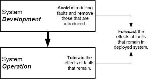
FIGURE 5.1 The four approaches to dealing with faults—avoidance, elimination, tolerance, and forecasting.
In practice, careful manufacturing and operational techniques permit many degradation faults to be ignored in computer systems. The rate of failure of modern microprocessors is so low that we rarely experience failures of the processors and memories in desktop machines. In part, this extraordinary reliability is the result of manufacturing techniques that avoid faults. Certainly we see failures of disks, power supplies, connectors, cooling fans, and circuit boards, and fault avoidance for these components has not progressed as far as fault avoidance in integrated circuits. These devices are dealt with using the other three approaches to dealing with faults.
5.2.2 Design Faults
For design faults, fault avoidance is entirely possible because of the basic notion of a design fault; something is wrong with the design. If we design a system with great care, we can, in fact, preclude the introduction of various classes of design faults. The way that this is done is by the use of systematic design techniques in which certain faults are precluded by the nature of the technique.
As far as software is concerned, faults can enter at any stage in the lifecycle. To avoid software faults, avoidance techniques have to be applied, therefore, at every stage. We will examine two important techniques for fault avoidance in Chapter 8 and Chapter 9. Here we look at a simple example to illustrate the idea.
A common example of software fault avoidance is to preclude certain constructs and to require others in high-level-language programs. These rules are often so simple that they can be checked by compilers or similar tools. Here are some simple cases:
Initialize all variables in a prescribed program location. If all variables are initialized to a known value, errors such as non-determinism and erroneous calculation associated with uninitialized-variable faults can be completely avoided. A typical location for such initialization is immediately after declaration.
Always include an else clause in a case statement. There is no possibility of software failing because of a missing case if this rule is followed. The semantics of case statements differ in different languages, and engineers can easily get confused.
Similar rules to these apply to hardware. Software rules are often developed in significant numbers in what are often called style guides to try to avoid faults of many types. An example is Ada 95 Quality and Style: Guidelines for Professional Programmers [34]. This is a comprehensive guide to developing software in Ada, and the text contains many hundreds of guidelines in all areas of the language. Such standards are discussed in Section 9.4.
5.3 Fault Elimination
Fault elimination is the active examination of a system to locate faults and to remove them. Fault elimination is conducted prior to the deployment of a system since the necessary examination cannot really be carried out with a system in operation.
5.3.1 Degradation Faults
Elimination of degradation faults seems like a strange idea. Since fault elimination takes place for the most part before a system is deployed, how can degradation faults have arisen before deployment? There are two aspects to this, each of which might arise inadvertently:
• Defective components might have been used in the construction of the system, and these components need to be found and replaced.
• Components might have been used that are subject to infant mortality, and a period of performance designed to cause such components to fail is needed.
Thus, elimination of degradation faults is an important part of system development. Designers must be sure that all of the system’s components are functioning as expected prior to deployment, and they must be sure that the probabilities of degradation faults for the system’s components have dropped below the infant mortality rate.
5.3.2 Design Faults
Design faults are the major target of fault elimination. Since design faults do not arise spontaneously, they are present and unchanging from the point in time when they are introduced until they are actively removed. To seek out and eliminate design faults from a system during development is an essential activity. To eliminate a design fault, four critical steps are necessary:
• The presence of the fault has to be detected.
• The fault has to be identified.
• The fault has to be repaired.
• The resulting new design has to be verified so as to ensure that no new fault has been introduced as a result of the removal of the original fault.
The first three of these steps seem reasonably intuitive, but what about the fourth? Experience has shown that the repair of faults in software is often itself faulty. The changes made to software to correct a fault are actually incomplete or incorrect in some way, and often the effect is to create a false sense of security.
Design faults arise in all aspects of system design, and attempting to eliminate all of them is crucial. The most important class of design faults, however, is software faults, because they are the most common type of design fault and because they are so difficult to deal with. Much of the material in the latter parts of this book is concerned with the elimination of software faults.
5.4 Fault Tolerance
5.4.1 Familiarity with Fault Tolerance
Fault tolerance is a technique with which we are all familiar, because we come across examples regularly in our everyday lives. Examples include:
• Automobile spare tires allow us to deal with punctures, and dual braking systems provide some braking when the system loses brake fluid.
• Overdraft protection on bank accounts avoids checks being returned if the account balance drops below zero.
• Uninterruptable power supplies and power-fail interrupts for computer power sources allow action to be taken, such as safely saving files and logging off, when the primary source of power fails.
• Multiple engines on an aircraft allow safe flight to continue when an engine fails.
• Emergency lighting in buildings permits safe exit when the primary lighting systems fail.
• Backup copies of disk files provide protection against loss of data if the primary disk fails.
• Parity and Single-bit Error Correction Double-bit Error Detection (SECDED) in data storage and transmission allow some data errors to be detected (parity) or corrected (SECDED).
Although fairly simple, these examples illustrate the power that fault tolerance can have in helping to implement dependability.
5.4.2 Definitions
In order to enable a systematic and precise basis for the use of fault tolerance in computer systems, various authors have provided definitions of fault tolerance. Here are two definitions from the literature: Sieworek and Swarz [131]:
“Fault-tolerant computing is the correct execution of a specified algorithm in the presence of defects”
This definition is a useful start, but there are two things to note. First, “correct execution” does not necessarily mean that the system will provide the same service when faults manifest themselves. Second, “the presence of defects” does not mean all defects. Defects might arise for which correct execution is not possible. Both of these points should be clear in a definition like this.
Anderson and Lee, paraphrased [10]:
“The fault-tolerant approach accepts that an implemented system will not be perfect, and that measures are therefore required to enable the operational system to cope with the faults that remain or develop.”
This definition adds the explicit statement that a system will not be perfect, and this is a helpful reminder of what dependability is all about. Unfortunately, this definition also includes the phrase “the faults that remain or develop”, and there is an implication that a system which utilizes fault tolerance can cope with all of the faults that remain or develop. This is not the case. There is a second implication in this definition that the “measures” will be successful when called upon to operate. They might not be. Again, such implications should not be present, and any definition of fault tolerance should not make them.
These observations lead to the following definition that is derived from the two definitions above:
Fault tolerance: A system that incorporates a fault-tolerance mechanism is one that is intended to continue to provide acceptable service in the presence of some faults.
Although well meaning, this definition is still not what we want. All three of these definitions actually refer to a mechanism, not the underlying concept. Here is the definition from the taxonomy:
Fault tolerance: Fault tolerance means to avoid service failures in the presence of faults.
This definition is the correct one. Avoiding service failures does not imply identical service. That some faults will not be tolerated by a particular mechanism does not mean that the definition of the concept is wrong.
Fault tolerance is an attempt to increase the dependability of the computing system to which it is applied. Elements are added to the computing system that, in the absence of faults, do not affect the normal operation of the system.
Fault tolerance is a complex topic. Essentially, what we are asking a system to do is:
• Deal with a situation that is to a large extent unpredictable.
• Ensure that the external behavior of the system that we observe is acceptable, either because the service provided is identical to the service we would receive had the fault not manifested itself or because the service provided is acceptable to us in a predefined way.
• Do all of this automatically.
Achieving this functionality is a tall order.
The unpredictability of the situation arises from many sources. For an anticipated degradation fault, the manifestation of the fault will occur at an unpredictable time. We cannot know when a component will fail. For degradation faults that we do not anticipate, the error, the failure semantics, and the time of manifestation will all be unknown.
For design faults, the situation is yet more complex. By their very nature, we cannot anticipate design faults very well. We know that software faults are likely to occur, but we have no idea about:
• What form a software fault will take.
• Where within the software a fault will be located.
• What the failure semantics of a software fault will be.
If we knew that a software fault lay within a certain small section of code, we would examine that section of code carefully and eliminate the fault. If we knew that a software fault would always have simple failure semantics, e.g., the software would stop and not damage any external state, we could plan for such an event. In practice, neither of these conditions occurs.
In practice, all we know is that design faults might occur, and that we will know little about their nature. Design faults are, therefore, difficult to tolerate, and efforts to do so are only of limited success. We will examine this topic in more depth in Chapter 11.
For Byzantine faults, the basis of such faults is some form of hardware degradation coupled with a transmission mechanism of the state. As a result, Byzantine faults are somewhat amenable to fault tolerance. An immense amount of work on the subject has been conducted and several efficient and effective mechanisms have been developed for Byzantine faults. We will examine this topic in more depth in Section 5.7.
With these various difficulties in mind, we now proceed to examine some of the important principles of fault tolerance.
5.4.3 Semantics of Fault Tolerance
If a mechanism acts to cope with the effects of a fault that is manifested, what do we require the semantics of the mechanism to be? This question is crucial. The semantics we need vary from system to system, and different semantics differ in the difficulty and cost of their implementation. There are three major dimensions to the semantics of concern:
• The externally observed service provided by the system during the period of time that the fault-tolerance mechanism acts.
In some cases, any deviation from the planned service is unacceptable, in which case the fault-tolerance mechanism has to mask the effects of the fault. In other cases, the planned service can be replaced with a different service for some period of time.
• The externally observed service of the system after the fault-tolerance mechanism acts.
If long-term deviation from the planned service is unacceptable, the fault-tolerance mechanism has to ensure that the actions taken allow normal service to be continued. Otherwise, the planned service can be replaced with a different service. Maintaining the same service can be difficult primarily because of the resources that are needed.
• The time during which the service provided by the system will be different from the planned service.
If this time has to be zero, then the effects of the fault have to be masked. If not, then there will be an upper bound that has to be met.
5.4.4 Phases of Fault Tolerance
In order for a fault to be tolerated, no matter what type of fault is involved and no matter what the required semantics are, four basic actions are necessary: (1) the error has to be detected; (2) the extent of the error has to be determined; (3) the error has to be repaired; and (4) functionality has to be resumed using the repaired state. These actions are referred to as the four phases of fault tolerance:
| Error Detection. | Determination that the state is erroneous. |
| Damage Assessment. | Determination of that part of the state which is damaged. |
| State Restoration. | Removal of the erroneous part of the state and its replacement with a valid state. |
| Continued Service. | Provision of service using the valid state. |
The second and third phases together are sometimes referred to by the comprehensive term error recovery.
The way in which these phases operate varies considerable. For some systems, no interruption in service is acceptable, in which case the effects of a fault have to be masked. The detailed semantics of these four phases are discussed in detail in Section 5.4.3.
All fault tolerance mechanisms employ these four phases. In some cases, a mechanism might appear to deviate from them, but a careful examination will reveal that they are, in fact, all there, although perhaps in a degenerate form. An example of such a mechanism is a system that intentionally shuts down whenever an internal component fails. Such systems are sometimes called fail safe, and there does not appear to be any continued service. In fact, the continued service is the provision of a benign interface. Although there is no functionality, there is a precise and well-defined interface upon which other systems can rely.
With the four phases of fault tolerance, we could, in principle, tolerate any fault. If we knew that a fault might manifest itself, then we could tolerate the fault by detecting the ensuing error, determining the damage to the state, repairing the state, and then taking steps to provide continued service.
This statement is correct, but does not say anything about how we can implement the four phases. And therein lies the problem. All four phases are difficult to achieve for virtually any fault, and so a great deal of care is needed if we are to develop a mechanism that can tolerate a fault properly.
Despite the difficulty that we face in implementing the four phases, they do provide us with two valuable benefits. Specifically, the four phases provide us with:
• A model that can be used to guide the development of mechanisms.
• A framework for evaluation of any particular fault-tolerance mechanism.
In the remainder of this book, we will frame our discussions of fault tolerance using these four phases.
5.4.5 An Example Fault-Tolerant System
To see how the four phases of fault tolerance operate, we look at an example. One of the most widely used fault-tolerant system structures is known as triple modular redundancy or TMR. An example of TMR is shown in Figure 5.2. In this example, three processors are operated in parallel with each receiving the same input. Each computes an output, and the outputs are supplied to a voter. By comparing the three values, the voter chooses a value and supplies that value as the TMR system’s output. The TMR structure can be used for any type of component (processor, memory, disk, network link, etc.)
The faults that this TMR system can tolerate are degradation faults in the processors, including both permanent and transient faults (see Section 3.4). Transient faults can be caused by nuclear particles and cosmic rays impacting silicon devices.
Tolerating such transient faults is generally important but especially so for computers that have to operate in high-radiation environments.
Hardware degradation faults in processors are important, but there are many other classes of faults that will not be tolerated. Faults not tolerated include degradation faults in the input and output mechanisms, the voter and the power supplies, and all design faults.
Even within the class of processor degradation faults, TMR is limited. TMR can tolerate at most two permanent degradation faults that occur serially. In order to tolerate the second fault, the fault cannot arise until after the process of tolerating the first fault has been completed. This limitation is not especially severe. If degradation faults in the processors arise independently and with small probability p per unit time, then if tolerating a fault can be completed in one time unit, the probability that a second fault will occur so as to interfere with tolerating the first is of order p2.
TMR can tolerate an arbitrary sequence of transient faults provided (a) the hardware is not damaged by the cause of the transient fault and (b) each transient fault does not overlap the previous transient fault.
The four phases of fault tolerance are implemented in TMR as follows:
Error detection. Errors are detected by differences in the outputs that the triplicated processors compute. These differences are present because of a fault, but the limitation of TMR only being able to tolerate a single fault arises, in part, because of error detection. The occurrence of a single degradation fault means that only one processor will produce incorrect output values. Since the other two processors are fault free, the voter is able to detect the difference.

FIGURE 5.2 Triple Modular Redundancy and the phases of fault tolerance.
Damage assessment. The actual damage that occurs in processors when they fail is usually quite limited. In integrated circuits, for example, a single gate getting stuck at a fixed logic value is common. This can occur when one out of millions of transistors fails or when a single wire out of thousands in the circuit breaks. Outside of integrated circuits, a single wire in a single connector can fail. Despite these circumstances, TMR with triplicated processors does not have sufficient information to do other than assume that the entire processor has failed. So, in TMR, damage assessment is to diagnose the failure of an entire unit. Damage assessment is also, in part, the reason for TMR’s ability to tolerate only a single degradation fault. With this restriction, the voter will see two identical sets of outputs and a single set of outputs that differs from the other two. If two degradation faults were possible, then two processors that were faulty could supply identical incorrect outputs to the voter, thereby defeating damage assessment.
State restoration. State restoration is achieved by removing the faulty processor. Removal is achieved by the voter merely ignoring subsequent outputs. Given the assumption of a single degradation fault only, this approach to state restoration provides a valid state from which to continue.
Continued service. Continued service is provided by the remaining two processors. Since they are assumed to be fault free, their outputs can continue to be used. With just two remaining processors, the ability of the system to tolerate faults has been reduced even if in this state the system can continue to provide service.
Once a TMR system has removed one of the processors from the set of three in order to tolerate a single degradation fault, the system is able to tolerate a second degradation fault but with very limited continued service. Since two processors remain functional, a second fault in either will be detected by the voter. In this case, however, there is no way to determine which processor experienced the fault. Thus damage assessment is limited to assuming the entire system is in error and continued service has to be limited to cessation of output.
Note carefully that the ability of a TMR system to tolerate faults has dropped as the two permanent degradation faults are tolerated. These issues are discussed in more detail in Section 6.3.3.
5.5 Fault Forecasting
For any fault that we cannot avoid, eliminate, or tolerate, we have to use fault forecasting. The idea is to predict the effects of the faults and to decide whether those effects are acceptable. If failures could be shown to occur at a rate below some prescribed value, the stakeholders of the system might be prepared to operate the system anyway.
The complexity of fault forecasting is increased by the need to be concerned with both degradation and design faults. Throughout this book we examine everything about dependability with the different characteristics of these two fault types in mind. When attempting to estimate probabilities of failure of components, both fault types need to be considered. Not surprisingly, the two fault types present different challenges in fault forecasting.
5.5.1 Fault Forecasting Process
Fault forecasting requires that a precise process be followed, because, by choosing to deal with faults by forecasting, the developer is admitting that anticipated faults will cause failures during operation. The process that has to be followed is:
• A high degree of assurance that the faults in question cannot be avoided, eliminated, or tolerated in a cost-effective way has to be established.
• The consequences of failure for each of the faults has to be quantified and assessed.
• An accurate statistical model of the rate of occurrence of failures from each of the faults has to be established.
• The ensuing system risk has to be computed (see Section 2.7.4).
• The acceptability of the risk to the system’s stakeholders has to be determined.
Of the various elements in this process, by far the most difficult is the third step. Accurate statistical models of the type required are notoriously difficult to develop.
5.5.2 The Operating Environment
The issues in fault forecasting are not merely mathematical. The manifestation of faults is influenced considerably by the operating environment. The system under development will be used in an operational environment that must be modeled accurately if the rate of occurrence of failures is to be properly predicted.
In practice, the inputs that a system ends up facing are rarely exactly as expected. For degradation faults, the problem lies in the circumstances of the physical environment. Temperature, humidity, vibration, and physical trauma all affect the types and frequency of degradation faults that will be manifested yet they are difficult to predict.
The operating environment is central to the modeling of design faults, as we see in Section 5.5.4.
5.5.3 Degradation Faults
As we noted in Section 3.5, degradation faults are fairly familiar. The notation that they are stochastic is familiar also. Incandescent light bulbs burn out with some probability per unit time, and the manufacturer can estimate the mean time to failure of the company’s light bulbs by measuring a sample. A similar but enhanced approach to quantitative assessment can be applied to degradation faults in the physical components of a computer system. Those components are much more complex than a light bulb and cost a lot more, and so modeling enters the picture (see Section 12.2.3).
5.5.4 Design Faults
Unfortunately, quantitative modeling and therefore fault forecasting of design faults is much less familiar and much more difficult than fault forecasting of degradation faults. To see why, consider the following hypothetical program fragment:

In this fragment, a sensor is being read and an actuator setting is being calculated and written. At the heart of the fragment is a software fault. For a particular value of the actuator setting, the software will always fail but only for that particular value.
The fault is, of course, a design fault. The software will always fail if the actuator setting is this special value. Unlike degradation faults, there is nothing stochastic about this behavior. If the specific input value for which the software fails arises, then the software will fail; otherwise it will not.
The fact that design faults are not stochastic in the same sense as degradation faults raises the question of whether metrics such as probability of failure per unit time are meaningful for artifacts like software. To the users of a software system, the software seems to fail in a stochastic manner. Poor software fails more often than good software, and this behavior seems to be stochastic. The reason for this apparent dilemma is that, for design faults, the randomness is in the inputs that are presented to the system. Input values are usually stochastic, and, if particular inputs arise by chance, then the associated design faults are triggered by chance.
This effect is illustrated in Figure 5.3. In the figure, software is shown as being part of a larger system, and that larger system is shown operating in an environment. The larger system might be something like an embedded computer network used in an automobile, in which case the environment will be the driver and all of the elements of the automobile.

FIGURE 5.3 The basis for the stochastic analysis of design faults.
In the figure, the system contains a design fault and the software two design faults, and input is shown originating in the environment. In the automobile example, the design fault in the system might be a wiring defect in the sensor or actuator network. Various inputs are supplied to the software by the system after they are presented to the system by the environment. Two specific inputs are shown that will trigger the design faults in the software, and one specific input is shown that will trigger the design fault in the system.
The stochastic nature of failures that derive from these design faults arises in both cases from the randomness of the inputs arising from the environment, not the faults themselves. Thus modeling of the stochastic nature of failures with design faults has to start with models of the environment.
5.6 Applying the Four Approaches to Fault Treatment
The four approaches to dealing with faults differ in their applicability, degree of success, and cost, and the differences are most significant when comparing degradation faults and design faults. Engineers must keep in mind that each approach has a role to play, and that the selection of approaches used will be system dependent.
Fault avoidance should always be our priority, but avoidance is much harder to practice with degradation faults. The success of fault avoidance depends upon the developers’ ability to identify the faults to which the system is subject and to effect appropriate avoidance measures. The cost of fault avoidance is really the lowest since no resources are needed beyond identifying the fault classes of interest and seeking ways to avoid them.
Fault elimination is difficult with both design and degradation faults. Not only do the fault types have to be identified, but mechanisms are need to try to identify the faults that might need to be eliminated. And then the elimination process has to be conducted. The cost is higher than fault avoidance, because fault elimination is usually conducted in addition to fault avoidance.
Fault tolerance is much more difficult to apply to design faults than to degradation faults and tends to be less successful. The cost of fault tolerance is always high, because enabling a system to tolerate residual faults, no matter of what type, requires the addition of system components that are not otherwise required.
Finally, fault forecasting relies upon modeling of fault behavior and the associated failure semantics. This modeling is much more difficult for design faults than for degradation faults. Fault forecasting is the most expensive approach to dealing with faults, because the approach literally is to allow the system to fail at a rate deemed sufficiently small by the system’s stakeholders. System failures can be costly, hence our interest in dependability.
5.7 Dealing with Byzantine Faults
The basic idea of Byzantine faults was introduced in Section 3.7. Byzantine faults are subtle, difficult to avoid or tolerate, and can have serious consequences. Recognizing their existence and serious nature has also allowed a serious problem in distributed systems to be uncovered and solved.
Byzantine faults can occur in essentially any real system, and engineers must either show by some means that such faults cannot arise in their specific system or show how the effects of such faults will be tolerated.
In dealing with Byzantine faults, engineers must understand how complex the problem is. Being lulled into a false sense of security is common as is thinking that a solution one has derived is correct. The solution might be correct, but experience has shown that the majority of people are convinced by informal arguments that are, in fact, wrong. In this area, analyzing algorithms mathematically is important. Even with mathematics, the analysis can be very subtle, and there have been cases in which people were convinced by formal arguments that were, in fact, wrong.
A complete and detailed treatment of the topic is beyond the scope of this book, and the interested reader is referred to the research literature on the subject. Many approaches to tolerating Byzantine faults have been developed along with some approaches to avoiding them. The necessary mathematics for all of this has been completed by the authors of the papers, and so using established results is likely to be much more successful than trying to develop solutions oneself.
From the perspective of the software engineer, understanding these issues so as to gain a healthy respect for the problem is the key requirement.
5.7.1 The Byzantine Generals
The concept of Byzantine faults was first introduced by Lamport, Shostak, and Pease in what they called the Byzantine Generals Problem [83]. The problem is a clever explanation of the underlying idea and is worth repeating.
As shown in Figure 5.4, several divisions of the Byzantine army are camped outside an enemy city, and the generals — the commanders of the divisions — have to decide whether they should attack the city or retreat. The generals need to agree on what the strategy is going to be, attack or retreat, because if some attack and some retreat they will obviously be in trouble.
The generals can only communicate by sending messages to each other. Under normal circumstances this restriction would be dealt with easily, but the army has been infiltrated by traitors. Some generals are traitors, and these traitors will attempt to disrupt the process of reaching agreement.
The army has two goals:
• All loyal generals must decide on the same strategy.
• A small number of traitors must not cause loyal generals to agree on a bad strategy.
These goals are stated informally, and in order to see how they apply and how they can be met, the goals are restated more formally.
Consider the role of just a single general. The general’s goal is to get the message about the strategy that he has selected to all of the other generals whom we will refer to as lieutenants. The general and any number of the lieutenants might be traitors. The goal of this communication is for the commanding general to send an order to his n-1 lieutenants so as to ensure that:
| IC1: | All loyal lieutenants obey the same order. |
| IC2: | If the commanding general is loyal, then all loyal lieutenants obey the order he sends. |
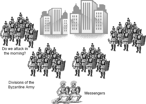
FIGURE 5.4 The Byzantine army surrounding an enemy city.
IC1 and IC2 are called the Interactive Consistency Conditions, and these conditions provide us with a formal statement that can both be the basis of seeking a solution and the basis of understanding the Byzantine Generals Problem as the problem applies to computers.
5.7.2 The Byzantine Generals and Computers
When one is initially presented with the Byzantine Generals Problem and the Interactive Consistency Conditions, one is tempted to ask what on Earth either has to do with computers. In particular, how could something this esoteric have anything to do with the dependability of computers? To see this, we need to refine the problem statement a little.
The relevance to dependable computing comes from the need to transmit data from one computer to another. The “general” is the computer that originates the transmission and the “lieutenants” are the receiving computers. In terms of computers, the Interactive Consistency Conditions become:
| IC1: | All non-faulty computers operate with the same data. |
| IC2: | If the originating computer is non-faulty, then all non-faulty receiving computers operate with the data sent by the originating computer. |

FIGURE 5.5 The Byzantine Generals Problem in a TMR system.
These conditions seems reasonable, perhaps even trivial in a sense. So, where are these conditions a problem and why should engineers care? The answers to these questions can be seen if we look at a simple triple-modular-redundant system, as shown in Figure 5.5. In a TMR system, the three different processors must operate with the same data if the system is to have the performance that is expected. If they operate with different data, then obviously the individual results of the different computers are likely to differ. In that case, the voter might conclude incorrectly that one or more processors has failed.
The problem seems to be limited to making sure that the input is distributed properly, and in a sense input distribution is the problem. Unfortunately, this distribution is far from simple. All the processors need to operate with the same input data, but they cannot be sure that the input distribution mechanism is not faulty. The obvious “solution” is to have the three processors exchange values, select a value to use if they are not identical, compare the values they received, and agree about which value they will use by some sort of selection process.
If the input source were the only problem, that would be fine. But the exchange of values by the processors is precisely the Byzantine Generals Problem. So we have to examine that carefully and make provision for the situation in which the processors themselves might be faulty.
The overall structure of the solution is to treat the input source as possibly faulty and accept that the three processors might have different data. The processors then need to reach a consensus about the value they will use in computation by undertaking some sort of algorithm that will allow the restated Interactive Consistency Conditions above to hold. Once this consensus is reached, the processors can continue with the application they are executing and know that the results presented to the voter by non-faulty processors will be the same.
There is just one problem with all this: there is no solution to the Byzantine Generals Problem if there are m traitors and no more than 3m generals. For the TMR case, what this means is that three processors cannot reach consensus as desired if one of them is faulty, i.e., the case m = 1.
This result is truly remarkable, because the result tells us that we have to be much more careful with redundant computer systems. Specifically:
• We must pay attention to Byzantine faults in such systems.
• We cannot distribute data as we need to in an N-modular redundant system (a generalization of triple-modular redundancy where N > 3) with m faulty computers unless N is greater than 3m.
An important discussion of the practical elements of the Byzantine Generals Problem was presented by Driscol et al [38]. The paper presents a discussion of how Byzantine faults arise in the analog electrical circuits used to implement digital functionality. Of special note are examples that illustrate clearly how specific instances of Byzantine behavior can arise and how the effects are propagated throughout complex electronics.
5.7.3 The Impossibility Result
Surely, if we look carefully, we can find an algorithm that will allow the processors in a TMR system to reach consensus. This is a tempting thought, but do not bother looking. There is no such algorithm. To see why, we need to look carefully at the TMR case, although things are a bit easier to follow if we go back to using generals and messages as the context.
We begin with the commander and two lieutenants, as shown in Figure 5.6. The commander transmits a message to the two lieutenants, and they exchange values so as to try to determine a consensus. As shown in Figure 5.6(a), lieutenant 1 sees “attack” from the commander and “retreat” from the other lieutenant. In order to be sure that he obeys IC2, lieutenant 1 must decide to “attack” because that is what he got from the commander. To do otherwise, irrespective of what lieutenant 2 claims, would mean the possibility of violating IC2 because lieutenant 1 cannot tell which of the other two participants is a traitor.

FIGURE 5.6 The inconsistency at the heart of the impossibility result.
Now consider how things look to lieutenant 2, as shown in Figure 5.6(b). In the case where he receives “retreat” from the commander, he too must obey this order or risk violating IC2. But by doing so, he violates IC1. In the case where the commander is a traitor, both lieutenants are required to do the same thing by IC1 and they do not. This surprising result can be generalized quite easily to the case of m traitors and 3m generals [83].
5.7.4 Solutions to the Byzantine Generals Problem
For 3m+1 generals including m traitors, a solution to the problem exists that is based purely on voting. The solution requires multiple rounds of data exchange and a fairly complicated vote.
An intriguing solution exists if generals are required to sign their messages. The solution works for 3m generals in the presence of m traitors so the solution bypasses the impossibility result. The solution with signed messages is a great advantage in practice, because the solution offers an approach to fixing the situation with TMR.
In this solution, generals are required to sign their messages, and two assumptions are introduced about the new type of messages:
• A loyal general’s signature cannot be forged, and any alteration of the contents of his signed message can be detected.
• Anyone can verify the authenticity of a general’s signature.
At first glance, these assumptions seem quite unrealistic. Since we are dealing with traitors who are prepared to lie, does that not mean that they would happily forge a signature? At this point the analogy with generals does us a disservice, because we are not thinking about what the computers (the things we care about) are doing.
The notion of lying derives from a failed computer failing to transmit a message with integrity. Because the computer is faulty, we cannot be sure what effect the computer’s fault might have on the content of a message. One thing we can assume is that the actions of a faulty computer are not malicious. So the idea of “lying” is not quite correct. The faulty computer is actually babbling in a way that we cannot predict.
What this means for signatures is that forging a signature will only occur with a very small probability. To forge a 32-bit signature, for example, would require a babbling computer to generate a valid signature by chance. If the computer were to generate a 32-bit string at random, the probability that the random string matched a signature would be 1 in 232, or about one in four billion.
The same argument applies to detection of a faulty computer’s possible changes to the message. The use of parity and other checks to make sure that the contents have not been changed randomly is both simple and effective. Thus, in practice, the extra two assumptions are quite reasonable, and the solution using signed messages can be used quite effectively.
Since the introduction of the Byzantine Generals Problem, variations on the different circumstances and assumptions have been developed along with many refined and special-purpose solutions.
Key points in this chapter:
♦ The four approaches to dealing with faults are avoidance, elimination, tolerance, and forecasting.
♦ The four approaches should be applied in order.
♦ All four approaches can be applied to all three fault types: degradation, design, and Byzantine.
♦ All fault-tolerance mechanisms operate in four steps: error detection, damage assessment, state restoration, and continued service.
♦ Byzantine faults can arise in a wide variety of computer systems.
♦ Byzantine faults are difficult to detect and tolerate.
♦ The impossibility result for Byzantine faults shows that three computers cannot tolerate a Byzantine fault; four are required.
Exercises
1. Explain the preferred order of applying the four approaches to fault treatment and explain why that order is preferred.
2. The notion of failure probability cannot be applied to a software system in the same way that it can be applied to a system subject to degradation faults. Explain why.
3. Explain how the notion of failure probability is applied to a software system.
4. Give examples of three instances of fault tolerance that you have seen in everyday life that are different from the list in Section 5.4.1.
5. For the programming language with which you are most familiar, search for a set of rules about programming designed to promote fault avoidance as discussed in Section 5.2.2.
6. What type of approach to dealing with faults is software testing? Explain your answer.
7. For a software fault in a program that you have written, document the fault and discuss the failure semantics of the fault.
8. For the software fault that is the subject of Exercise 7, discuss what would be needed to tolerate the fault during execution.
9. In general, degradation faults are easier to tolerate than design faults. Explain why this is the case.
10. The primary lighting systems in buildings are often supplemented by emergency lighting systems that come on when the primary system fails. The system is using fault tolerance to try to avoid service failures. For such a lighting system:
(a) Identify the four phases of fault tolerance in the lighting system.
(b) Determine the required semantics of fault tolerance in this case (see Section 5.4.3).
11. Locate the original paper that introduced the Byzantine Generals Problem [83], and explain the problem to a colleague.
12. Implement the voting algorithm contained in the original paper that introduced the Byzantine Generals Problem.
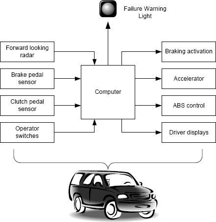
13. A sophisticated automobile cruise-control system provides automatic acceleration and braking to maintain speed equal to the vehicle ahead (if there is one) and a speed set by the driver otherwise. The system provides accident prevention by braking the car automatically if the system detects an imminent collision. If the system detects skidding during emergency braking, then the separate ABS is turned on. A variety of sensors monitor vehicle conditions, and a small radar monitors the vehicle ahead and attempts to locate obstacles ahead. A computer system provides all the various services. The system performs numerous self checks on the hardware whenever cruise control is not taking place. If a self-check fails, cruise control is disabled and a light is illuminated to inform the driver. The following figure illustrates the system design:
(a) Identify the hazards to which this system is subject.
(b) The failure semantics of the hardware sensors on the brake and clutch pedals are complex. When failed, they operate intermittently, and their behavior is inconsistent. These circumstances are common with degradation faults. What might the software monitoring these sensors do to try to detect the failures?
(c) What algorithms might the system employ in its self-checking process to detect faults in the brake activation and accelerator control mechanisms?
(d) Software failure of this system could be catastrophic, because the system has control of the accelerator and brakes. What checks might the software put into effect to detect its own failure in order to avoid excessive speed or braking? (Hint: whatever the software does, the commands to the accelerator and brakes should be “reasonable”.)