
Categorizing a data set and applying a function to each group, whether
an aggregation or transformation, is often a critical component of a data
analysis workflow. After loading, merging, and preparing a data set, a
familiar task is to compute group statistics or possibly pivot
tables for reporting or visualization purposes. pandas provides a
flexible and high-performance groupby
facility, enabling you to slice and dice, and summarize data sets in a
natural way.
One reason for the popularity of relational databases and SQL (which stands for “structured query language”) is the ease with which data can be joined, filtered, transformed, and aggregated. However, query languages like SQL are rather limited in the kinds of group operations that can be performed. As you will see, with the expressiveness and power of Python and pandas, we can perform much more complex grouped operations by utilizing any function that accepts a pandas object or NumPy array. In this chapter, you will learn how to:
Split a pandas object into pieces using one or more keys (in the form of functions, arrays, or DataFrame column names)
Computing group summary statistics, like count, mean, or standard deviation, or a user-defined function
Apply a varying set of functions to each column of a DataFrame
Apply within-group transformations or other manipulations, like normalization, linear regression, rank, or subset selection
Compute pivot tables and cross-tabulations
Perform quantile analysis and other data-derived group analyses
Note
Aggregation of time series data, a special use case of groupby, is referred to as
resampling in this book and will receive separate
treatment in Chapter 10.
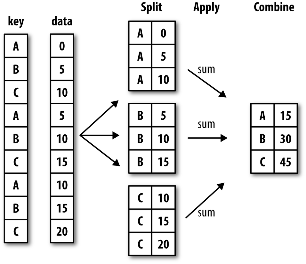
Hadley Wickham, an author of many popular packages for the R
programming language, coined the term split-apply-combine for talking about
group operations, and I think that’s a good description of the process. In
the first stage of the process, data contained in a pandas object, whether
a Series, DataFrame, or otherwise, is split into
groups based on one or more keys that you provide.
The splitting is performed on a particular axis of an object. For example,
a DataFrame can be grouped on its rows (axis=0) or its columns (axis=1). Once this is done, a function is
applied to each group, producing a new value.
Finally, the results of all those function applications are
combined into a result object. The form of the
resulting object will usually depend on what’s being done to the data. See
Figure 9-1 for a mockup of a simple group
aggregation.
Each grouping key can take many forms, and the keys do not have to be all of the same type:
A list or array of values that is the same length as the axis being grouped
A value indicating a column name in a DataFrame
A dict or Series giving a correspondence between the values on the axis being grouped and the group names
A function to be invoked on the axis index or the individual labels in the index
Note that the latter three methods are all just shortcuts for producing an array of values to be used to split up the object. Don’t worry if this all seems very abstract. Throughout this chapter, I will give many examples of all of these methods. To get started, here is a very simple small tabular dataset as a DataFrame:
In [160]: df = DataFrame({'key1' : ['a', 'a', 'b', 'b', 'a'],
   .....:                 'key2' : ['one', 'two', 'one', 'two', 'one'],
   .....:                 'data1' : np.random.randn(5),
   .....:                 'data2' : np.random.randn(5)})

In [161]: df
Out[161]:
      data1     data2 key1 key2
0 -0.204708  1.393406    a  one
1  0.478943  0.092908    a  two
2 -0.519439  0.281746    b  one
3 -0.555730  0.769023    b  two
4  1.965781  1.246435    a  one
Suppose you wanted to compute the mean of the data1 column using the groups labels from
key1. There are a number of ways to do
this. One is to access data1 and call
groupby with the column (a Series) at
key1:
In [162]: grouped = df['data1'].groupby(df['key1'])

In [163]: grouped
Out[163]: <pandas.core.groupby.SeriesGroupBy object at 0x7f5893ec7750>
This grouped variable is now a
GroupBy object. It has not actually computed anything
yet except for some intermediate data about the group key df['key1']. The idea is that this object has all
of the information needed to then apply some operation to each of the
groups. For example, to compute group means we can call the GroupBy’s
mean method:
In [164]: grouped.mean()
Out[164]:
key1
a       0.746672
b      -0.537585
Name: data1, dtype: float64
Later, I’ll explain more about what’s going on when you call
.mean(). The important
thing here is that the data (a Series) has been aggregated according to
the group key, producing a new Series that is now indexed by the unique
values in the key1 column. The result
index has the name 'key1' because the
DataFrame column df['key1'] did.
If instead we had passed multiple arrays as a list, we get something different:
In [165]: means = df['data1'].groupby([df['key1'], df['key2']]).mean()

In [166]: means
Out[166]:
key1  key2
a     one     0.880536
      two     0.478943
b     one    -0.519439
      two    -0.555730
Name: data1, dtype: float64
In this case, we grouped the data using two keys, and the resulting Series now has a hierarchical index consisting of the unique pairs of keys observed:
In [167]: means.unstack()
Out[167]:
key2       one       two
key1
a     0.880536  0.478943
b    -0.519439 -0.555730
In these examples, the group keys are all Series, though they could be any arrays of the right length:
In [168]: states = np.array(['Ohio', 'California', 'California', 'Ohio', 'Ohio'])

In [169]: years = np.array([2005, 2005, 2006, 2005, 2006])

In [170]: df['data1'].groupby([states, years]).mean()
Out[170]:
California  2005    0.478943
            2006   -0.519439
Ohio        2005   -0.380219
            2006    1.965781
Name: data1, dtype: float64
Frequently the grouping information to be found in the same DataFrame as the data you want to work on. In that case, you can pass column names (whether those are strings, numbers, or other Python objects) as the group keys:
In [171]: df.groupby('key1').mean()
Out[171]:
         data1     data2
key1
a     0.746672  0.910916
b    -0.537585  0.525384

In [172]: df.groupby(['key1', 'key2']).mean()
Out[172]:
              data1     data2
key1 key2
a    one   0.880536  1.319920
     two   0.478943  0.092908
b    one  -0.519439  0.281746
     two  -0.555730  0.769023
You may have noticed in the first case df.groupby('key1').mean() that there is no
key2 column in the result. Because
df['key2'] is not numeric data, it is
said to be a nuisance column, which is therefore
excluded from the result. By default, all of the numeric columns are aggregated, though it is
possible to filter down to a subset as you’ll see soon.
Regardless of the objective in using groupby, a generally useful GroupBy method is
size which return a
Series containing group sizes:
In [173]: df.groupby(['key1', 'key2']).size()
Out[173]:
key1  key2
a     one     2
      two     1
b     one     1
      two     1
dtype: int64
Caution
As of this writing, any missing values in a group key will be
excluded from the result. It’s possible (and, in fact, quite likely),
that by the time you are reading this there will be an option to include
the NA group in the result.
The GroupBy object supports iteration, generating a sequence of 2-tuples containing the group name along with the chunk of data. Consider the following small example data set:
In [174]: for name, group in df.groupby('key1'):
   .....:     print(name)
   .....:     print(group)
   .....:
a
      data1     data2 key1 key2
0 -0.204708  1.393406    a  one
1  0.478943  0.092908    a  two
4  1.965781  1.246435    a  one
b
      data1     data2 key1 key2
2 -0.519439  0.281746    b  one
3 -0.555730  0.769023    b  two
In the case of multiple keys, the first element in the tuple will be a tuple of key values:
In [175]: for (k1, k2), group in df.groupby(['key1', 'key2']):
   .....:     print((k1, k2))
   .....:     print(group)
   .....:
a one
      data1     data2 key1 key2
0 -0.204708  1.393406    a  one
4  1.965781  1.246435    a  one
a two
      data1     data2 key1 key2
1  0.478943  0.092908    a  two
b one
      data1     data2 key1 key2
2 -0.519439  0.281746    b  one
b two
     data1     data2 key1 key2
3 -0.55573  0.769023    b  two
Of course, you can choose to do whatever you want with the pieces of data. A recipe you may find useful is computing a dict of the data pieces as a one-liner:
In [176]: pieces = dict(list(df.groupby('key1')))

In [177]: pieces['b']
Out[177]:
      data1     data2 key1 key2
2 -0.519439  0.281746    b  one
3 -0.555730  0.769023    b  two
By default groupby groups on
axis=0, but you can group on any of
the other axes. For example, we could group the columns of our example
df here by dtype like so:
In [178]: df.dtypes
Out[178]:
data1    float64
data2    float64
key1      object
key2      object
dtype: object

In [179]: grouped = df.groupby(df.dtypes, axis=1)

In [180]: dict(list(grouped))
Out[180]:
{dtype('float64'):       data1     data2
 0 -0.204708  1.393406
 1  0.478943  0.092908
 2 -0.519439  0.281746
 3 -0.555730  0.769023
 4  1.965781  1.246435, dtype('O'):   key1 key2
 0    a  one
 1    a  two
 2    b  one
 3    b  two
4 a one}Indexing a GroupBy object created from a DataFrame with a column name or array of column names has the effect of selecting those columns for aggregation. This means that:
df.groupby('key1')['data1']
df.groupby('key1')[['data2']]
are syntactic sugar for:
df['data1'].groupby(df['key1'])
df[['data2']].groupby(df['key1'])
Especially for large data sets, it may be desirable to aggregate
only a few columns. For example, in the above data set, to compute means
for just the data2 column and get the
result as a DataFrame, we could write:
In [181]: df.groupby(['key1', 'key2'])[['data2']].mean()
Out[181]:
              data2
key1 key2
a    one   1.319920
     two   0.092908
b    one   0.281746
     two   0.769023
The object returned by this indexing operation is a grouped DataFrame if a list or array is passed and a grouped Series is just a single column name that is passed as a scalar:
In [182]: s_grouped = df.groupby(['key1', 'key2'])['data2']

In [183]: s_grouped
Out[183]: <pandas.core.groupby.SeriesGroupBy object at 0x7f5893e77890>

In [184]: s_grouped.mean()
Out[184]:
key1  key2
a     one     1.319920
      two     0.092908
b     one     0.281746
      two     0.769023
Name: data2, dtype: float64
Grouping information may exist in a form other than an array. Let’s consider another example DataFrame:
In [185]: people = DataFrame(np.random.randn(5, 5),
   .....:                    columns=['a', 'b', 'c', 'd', 'e'],
   .....:                    index=['Joe', 'Steve', 'Wes', 'Jim', 'Travis'])

In [186]: people.ix[2:3, ['b', 'c']] = np.nan # Add a few NA values

In [187]: people
Out[187]:
               a         b         c         d         e
Joe     1.007189 -1.296221  0.274992  0.228913  1.352917
Steve   0.886429 -2.001637 -0.371843  1.669025 -0.438570
Wes    -0.539741       NaN       NaN -1.021228 -0.577087
Jim     0.124121  0.302614  0.523772  0.000940  1.343810
Travis -0.713544 -0.831154 -2.370232 -1.860761 -0.860757
Now, suppose I have a group correspondence for the columns and want to sum together the columns by group:
In [188]: mapping = {'a': 'red', 'b': 'red', 'c': 'blue',
   .....:            'd': 'blue', 'e': 'red', 'f' : 'orange'}
Now, you could easily construct an array from this dict to pass to
groupby, but instead we can just pass
the dict:
In [189]: by_column = people.groupby(mapping, axis=1)

In [190]: by_column.sum()
Out[190]:
            blue       red
Joe     0.503905  1.063885
Steve   1.297183 -1.553778
Wes    -1.021228 -1.116829
Jim     0.524712  1.770545
Travis -4.230992 -2.405455
The same functionality holds for Series, which can be viewed as a fixed size mapping. When I used Series as group keys in the above examples, pandas does, in fact, inspect each Series to ensure that its index is aligned with the axis it’s grouping:
In [191]: map_series = Series(mapping)

In [192]: map_series
Out[192]:
a       red
b       red
c      blue
d      blue
e       red
f    orange
dtype: object

In [193]: people.groupby(map_series, axis=1).count()
Out[193]:
        blue  red
Joe        2    3
Steve      2    3
Wes        1    2
Jim        2    3
Travis 2 3Using Python functions in what can be fairly creative ways
is a more abstract way of defining a group mapping compared with a dict
or Series. Any function passed as a group key will be called once per
index value, with the return values being used as the group names. More
concretely, consider the example DataFrame from the previous section,
which has people’s first names as index values. Suppose you wanted to
group by the length of the names; you could compute an array of string
lengths, but instead you can just pass the len function:
In [194]: people.groupby(len).sum()
Out[194]:
          a         b         c         d         e
3  0.591569 -0.993608  0.798764 -0.791374  2.119639
5  0.886429 -2.001637 -0.371843  1.669025 -0.438570
6 -0.713544 -0.831154 -2.370232 -1.860761 -0.860757
Mixing functions with arrays, dicts, or Series is not a problem as everything gets converted to arrays internally:
In [195]: key_list = ['one', 'one', 'one', 'two', 'two']

In [196]: people.groupby([len, key_list]).min()
Out[196]:
              a         b         c         d         e
3 one -0.539741 -1.296221  0.274992 -1.021228 -0.577087
  two  0.124121  0.302614  0.523772  0.000940  1.343810
5 one  0.886429 -2.001637 -0.371843  1.669025 -0.438570
6 two -0.713544 -0.831154 -2.370232 -1.860761 -0.860757A final convenience for hierarchically-indexed data sets
is the ability to aggregate using one of the levels of an axis index. To
do this, pass the level number or name using the level
keyword:
In [197]: columns = pd.MultiIndex.from_arrays([['US', 'US', 'US', 'JP', 'JP'],
   .....:                                     [1, 3, 5, 1, 3]], names=['cty', 'tenor'])

In [198]: hier_df = DataFrame(np.random.randn(4, 5), columns=columns)

In [199]: hier_df
Out[199]:
cty          US                            JP
tenor         1         3         5         1         3
0      0.560145 -1.265934  0.119827 -1.063512  0.332883
1     -2.359419 -0.199543 -1.541996 -0.970736 -1.307030
2      0.286350  0.377984 -0.753887  0.331286  1.349742
3      0.069877  0.246674 -0.011862  1.004812  1.327195

In [200]: hier_df.groupby(level='cty', axis=1).count()
Out[200]:
cty  JP  US
0     2   3
1     2   3
2     2   3
3     2   3
By aggregation, I am generally referring to any data
transformation that produces scalar values from arrays. In the examples
above I have used several of them, such as mean,
count, min and sum. You may wonder what
is going on when you invoke mean() on a GroupBy
object. Many common aggregations, such as those found in Table 9-1, have optimized implementations
that compute the statistics on the dataset in place.
However, you are not limited to only this set of methods. You can use
aggregations of your own devising and additionally call any method that is
also defined on the grouped object. For example, as you recall quantile computes sample quantiles of a Series
or a DataFrame’s columns [3]:
In [201]: df
Out[201]:
      data1     data2 key1 key2
0 -0.204708  1.393406    a  one
1  0.478943  0.092908    a  two
2 -0.519439  0.281746    b  one
3 -0.555730  0.769023    b  two
4  1.965781  1.246435    a  one

In [202]: grouped = df.groupby('key1')

In [203]: grouped['data1'].quantile(0.9)
Out[203]:
key1
a       1.668413
b      -0.523068
Name: data1, dtype: float64
While quantile is not explicitly
implemented for GroupBy, it is a Series method and thus available for use.
Internally, GroupBy efficiently slices up the Series, calls piece.quantile(0.9) for each piece, then
assembles those results together into the result object.
To use your own aggregation functions, pass any function that
aggregates an array to the aggregate or agg method:
In [204]: def peak_to_peak(arr):
   .....:     return arr.max() - arr.min()

In [205]: grouped.agg(peak_to_peak)
Out[205]:
         data1     data2
key1
a     2.170488  1.300498
b     0.036292  0.487276
You’ll notice that some methods like describe also work, even though they are not
aggregations, strictly speaking:
In [206]: grouped.describe()
Out[206]:
               data1     data2
key1
a    count  3.000000  3.000000
     mean   0.746672  0.910916
     std    1.109736  0.712217
     min   -0.204708  0.092908
     25%    0.137118  0.669671
...              ...       ...
b    min   -0.555730  0.281746
     25%   -0.546657  0.403565
     50%   -0.537585  0.525384
     75%   -0.528512  0.647203
     max   -0.519439  0.769023
[16 rows x 2 columns]
I will explain in more detail what has happened here in the next major section on group-wise operations and transformations.
Note
You may notice that custom aggregation functions are much slower than the optimized functions found in Table 9-1. This is because there is significant overhead (function calls, data rearrangement) in constructing the intermediate group data chunks.
Table 9-1. Optimized groupby methods
To illustrate some more advanced aggregation features, I’ll use a
less trivial dataset, a dataset on restaurant tipping. I obtained it from
the R reshape2 package; it was
originally found in Bryant & Smith’s 1995 text on business statistics
(and found in the book’s GitHub repository). After loading it with
read_csv, I add a tipping
percentage column tip_pct.
In [207]: tips = pd.read_csv('ch08/tips.csv')

# Add tip percentage of total bill
In [208]: tips['tip_pct'] = tips['tip'] / tips['total_bill']

In [209]: tips[:6]
Out[209]:
   total_bill   tip     sex smoker  day    time  size   tip_pct
0       16.99  1.01  Female     No  Sun  Dinner     2  0.059447
1       10.34  1.66    Male     No  Sun  Dinner     3  0.160542
2       21.01  3.50    Male     No  Sun  Dinner     3  0.166587
3       23.68  3.31    Male     No  Sun  Dinner     2  0.139780
4       24.59  3.61  Female     No  Sun  Dinner     4  0.146808
5 25.29 4.71 Male No Sun Dinner 4 0.186240As you’ve seen above, aggregating a Series or all of the
columns of a DataFrame is a matter of using aggregate with the
desired function or calling a method like mean or std. However, you may want to aggregate using
a different function depending on the column or multiple functions at
once. Fortunately, this is straightforward to do, which I’ll illustrate
through a number of examples. First, I’ll group the tips by sex
and smoker:
In [210]: grouped = tips.groupby(['sex', 'smoker'])
Note that for descriptive statistics like those in Table 9-1, you can pass the name of the function as a string:
In [211]: grouped_pct = grouped['tip_pct']

In [212]: grouped_pct.agg('mean')
Out[212]:
sex     smoker
Female  No        0.156921
        Yes       0.182150
Male    No        0.160669
        Yes       0.152771
Name: tip_pct, dtype: float64
If you pass a list of functions or function names instead, you get back a DataFrame with column names taken from the functions:
In [213]: grouped_pct.agg(['mean', 'std', peak_to_peak])
Out[213]:
                   mean       std  peak_to_peak
sex    smoker
Female No      0.156921  0.036421      0.195876
       Yes     0.182150  0.071595      0.360233
Male   No      0.160669  0.041849      0.220186
       Yes     0.152771  0.090588      0.674707
You don’t need to accept the names that GroupBy gives to the
columns; notably lambda functions have
the name '<lambda>' which make
them hard to identify (you can see for yourself by looking at a
function’s __name__ attribute). As
such, if you pass a list of (name,
function) tuples, the first element of each tuple will be used
as the DataFrame column names (you can think of a list of 2-tuples as an
ordered mapping):
In [214]: grouped_pct.agg([('foo', 'mean'), ('bar', np.std)])
Out[214]:
                    foo       bar
sex    smoker
Female No      0.156921  0.036421
       Yes     0.182150  0.071595
Male   No      0.160669  0.041849
       Yes     0.152771  0.090588
With a DataFrame, you have more options as you can specify a list
of functions to apply to all of the columns or different functions per
column. To start, suppose we wanted to compute the same three statistics
for the tip_pct and total_bill columns:
In [215]: functions = ['count', 'mean', 'max']

In [216]: result = grouped['tip_pct', 'total_bill'].agg(functions)

In [217]: result
Out[217]:
               tip_pct                      total_bill
                 count      mean       max       count       mean    max
sex    smoker
Female No           54  0.156921  0.252672          54  18.105185  35.83
       Yes          33  0.182150  0.416667          33  17.977879  44.30
Male   No           97  0.160669  0.291990          97  19.791237  48.33
       Yes          60  0.152771  0.710345          60  22.284500  50.81
As you can see, the resulting DataFrame has hierarchical columns,
the same as you would get aggregating each column separately and using
concat to glue the results together
using the column names as the keys
argument:
In [218]: result['tip_pct']
Out[218]:
               count      mean       max
sex    smoker
Female No         54  0.156921  0.252672
       Yes        33  0.182150  0.416667
Male   No         97  0.160669  0.291990
       Yes        60  0.152771  0.710345
As above, a list of tuples with custom names can be passed:
In [219]: ftuples = [('Durchschnitt', 'mean'), ('Abweichung', np.var)]

In [220]: grouped['tip_pct', 'total_bill'].agg(ftuples)
Out[220]:
                    tip_pct                total_bill
               Durchschnitt  Abweichung  Durchschnitt  Abweichung
sex    smoker
Female No          0.156921    0.001327     18.105185   53.092422
       Yes         0.182150    0.005126     17.977879   84.451517
Male   No          0.160669    0.001751     19.791237   76.152961
       Yes         0.152771    0.008206     22.284500   98.244673
Now, suppose you wanted to apply potentially different functions
to one or more of the columns. The trick is to pass a dict to agg that contains a mapping of column names to
any of the function specifications listed so far:
In [221]: grouped.agg({'tip' : np.max, 'size' : 'sum'})
Out[221]:
                tip  size
sex    smoker
Female No       5.2   140
       Yes      6.5    74
Male   No       9.0   263
       Yes     10.0   150

In [222]: grouped.agg({'tip_pct' : ['min', 'max', 'mean', 'std'],
   .....:              'size' : 'sum'})
Out[222]:
                tip_pct                                size
                    min       max      mean       std   sum
sex    smoker
Female No      0.056797  0.252672  0.156921  0.036421   140
       Yes     0.056433  0.416667  0.182150  0.071595    74
Male   No      0.071804  0.291990  0.160669  0.041849   263
       Yes     0.035638  0.710345  0.152771  0.090588   150
A DataFrame will have hierarchical columns only if multiple functions are applied to at least one column.
In all of the examples up until now, the aggregated data
comes back with an index, potentially hierarchical, composed from the
unique group key combinations observed. Since this isn’t always
desirable, you can disable this behavior in most cases by passing
as_index=False to groupby:
In [223]: tips.groupby(['sex', 'smoker'], as_index=False).mean()
Out[223]:
      sex smoker  total_bill       tip      size   tip_pct
0  Female     No   18.105185  2.773519  2.592593  0.156921
1  Female    Yes   17.977879  2.931515  2.242424  0.182150
2    Male     No   19.791237  3.113402  2.711340  0.160669
3    Male    Yes   22.284500  3.051167  2.500000  0.152771
Of course, it’s always possible to obtain the result in this
format by calling reset_index on the
result.
Aggregation is only one kind of group operation. It is a special
case in the more general class of data transformations; that is, it
accepts functions that reduce a one-dimensional array to a scalar value.
In this section, I will introduce you to the transform and apply methods, which will enable you to do many
other kinds of group operations.
Suppose, instead, we wanted to add a column to a DataFrame containing group means for each index. One way to do this is to aggregate, then merge:
In [224]: df
Out[224]:
      data1     data2 key1 key2
0 -0.204708  1.393406    a  one
1  0.478943  0.092908    a  two
2 -0.519439  0.281746    b  one
3 -0.555730  0.769023    b  two
4  1.965781  1.246435    a  one

In [225]: k1_means = df.groupby('key1').mean().add_prefix('mean_')

In [226]: k1_means
Out[226]:
      mean_data1  mean_data2
key1
a       0.746672    0.910916
b      -0.537585    0.525384

In [227]: pd.merge(df, k1_means, left_on='key1', right_index=True)
Out[227]:
      data1     data2 key1 key2  mean_data1  mean_data2
0 -0.204708  1.393406    a  one    0.746672    0.910916
1  0.478943  0.092908    a  two    0.746672    0.910916
4  1.965781  1.246435    a  one    0.746672    0.910916
2 -0.519439  0.281746    b  one   -0.537585    0.525384
3 -0.555730  0.769023    b  two   -0.537585    0.525384
This works, but is somewhat inflexible. You can think of the
operation as transforming the two data columns using the np.mean function. Let’s
look back at the people DataFrame from
earlier in the chapter and use the transform method on GroupBy:
In [228]: key = ['one', 'two', 'one', 'two', 'one']

In [229]: people.groupby(key).mean()
Out[229]:
            a         b         c         d         e
one -0.082032 -1.063687 -1.047620 -0.884358 -0.028309
two  0.505275 -0.849512  0.075965  0.834983  0.452620

In [230]: people.groupby(key).transform(np.mean)
Out[230]:
               a         b         c         d         e
Jim          NaN       NaN       NaN       NaN       NaN
Joe          NaN       NaN       NaN       NaN       NaN
Steve        NaN       NaN       NaN       NaN       NaN
Travis       NaN       NaN       NaN       NaN       NaN
Wes          NaN       NaN       NaN       NaN       NaN
one    -0.082032 -1.063687 -1.047620 -0.884358 -0.028309
two     0.505275 -0.849512  0.075965  0.834983  0.452620
As you may guess, transform
applies a function to each group, then places the results in the
appropriate locations. If each group produces a scalar value, it will be
propagated (broadcasted). Suppose instead you wanted to subtract the mean
value from each group. To do this, create a demeaning function and pass it
to transform:
In [231]: def demean(arr):
   .....:     return arr - arr.mean()

In [232]: demeaned = people.groupby(key).transform(demean)

In [233]: demeaned
Out[233]:
               a         b         c         d         e
Jim    -0.381154  1.152125  0.447807 -0.834043  0.891190
Joe     1.089221 -0.232534  1.322612  1.113271  1.381226
Steve   0.381154 -1.152125 -0.447807  0.834043 -0.891190
Travis -0.631512  0.232534 -1.322612 -0.976402 -0.832448
Wes    -0.457709       NaN       NaN -0.136869 -0.548778
You can check that demeaned now
has zero group means:
In [234]: demeaned.groupby(key).mean()
Out[234]:
            a             b  c         d         e
one -0.152570  0.000000e+00  0 -0.045623 -0.182926
two  0.228855 -1.110223e-16  0  0.068435  0.274389
As you’ll see in the next section, group demeaning can be achieved
using apply also.
Like aggregate,
transform is a more specialized function
having rigid requirements: the passed function must either produce a
scalar value to be broadcasted (like np.mean) or a transformed array of the same
size. The most general purpose GroupBy method is apply, which is the subject of the rest of
this section. As in Figure 9-1, apply splits the object being manipulated into
pieces, invokes the passed function on each piece, then attempts to
concatenate the pieces together.
Returning to the tipping data set above, suppose you wanted to
select the top five tip_pct values by
group. First, it’s straightforward to write a function that selects the
rows with the largest values in a particular column:
In [235]: def top(df, n=5, column='tip_pct'):
   .....:     return df.sort_index(by=column)[-n:]

In [236]: top(tips, n=6)
Out[236]:
     total_bill   tip     sex smoker  day    time  size   tip_pct
109       14.31  4.00  Female    Yes  Sat  Dinner     2  0.279525
183       23.17  6.50    Male    Yes  Sun  Dinner     4  0.280535
232       11.61  3.39    Male     No  Sat  Dinner     2  0.291990
67         3.07  1.00  Female    Yes  Sat  Dinner     1  0.325733
178        9.60  4.00  Female    Yes  Sun  Dinner     2  0.416667
172        7.25  5.15    Male    Yes  Sun  Dinner     2  0.710345
Now, if we group by smoker,
say, and call apply with this
function, we get the following:
In [237]: tips.groupby('smoker').apply(top)
Out[237]:
            total_bill   tip     sex smoker   day    time  size   tip_pct
smoker
No     88        24.71  5.85    Male     No  Thur   Lunch     2  0.236746
       185       20.69  5.00    Male     No   Sun  Dinner     5  0.241663
       51        10.29  2.60  Female     No   Sun  Dinner     2  0.252672
       149        7.51  2.00    Male     No  Thur   Lunch     2  0.266312
       232       11.61  3.39    Male     No   Sat  Dinner     2  0.291990
Yes    109       14.31  4.00  Female    Yes   Sat  Dinner     2  0.279525
       183       23.17  6.50    Male    Yes   Sun  Dinner     4  0.280535
       67         3.07  1.00  Female    Yes   Sat  Dinner     1  0.325733
       178        9.60  4.00  Female    Yes   Sun  Dinner     2  0.416667
       172        7.25  5.15    Male    Yes   Sun  Dinner     2  0.710345
What has happened here? The top function is called
on each piece of the DataFrame, then the results are glued together
using pandas.concat, labeling
the pieces with the group names. The result therefore has a hierarchical
index whose inner level contains index values from the original
DataFrame.
If you pass a function to apply
that takes other arguments or keywords, you can pass these after the
function:
In [238]: tips.groupby(['smoker', 'day']).apply(top, n=1, column='total_bill')
Out[238]:
                 total_bill    tip     sex smoker   day    time  size
smoker day
No     Fri  94        22.75   3.25  Female     No   Fri  Dinner     2
       Sat  212       48.33   9.00    Male     No   Sat  Dinner     4
       Sun  156       48.17   5.00    Male     No   Sun  Dinner     6
       Thur 142       41.19   5.00    Male     No  Thur   Lunch     5
Yes    Fri  95        40.17   4.73    Male    Yes   Fri  Dinner     4
       Sat  170       50.81  10.00    Male    Yes   Sat  Dinner     3
       Sun  182       45.35   3.50    Male    Yes   Sun  Dinner     3
       Thur 197       43.11   5.00  Female    Yes  Thur   Lunch     4
                  tip_pct
smoker day
No     Fri  94   0.142857
       Sat  212  0.186220
       Sun  156  0.103799
       Thur 142  0.121389
Yes    Fri  95   0.117750
       Sat  170  0.196812
       Sun  182  0.077178
       Thur 197  0.115982
Note
Beyond these basic usage mechanics, getting the most out of
apply is largely a matter of
creativity. What occurs inside the function passed is up to you; it
only needs to return a pandas object or a scalar value. The rest of
this chapter will mainly consist of examples showing you how to solve
various problems using groupby.
You may recall above I called describe on a GroupBy
object:
In [239]: result = tips.groupby('smoker')['tip_pct'].describe()

In [240]: result
Out[240]:
smoker
No      count    151.000000
        mean       0.159328
        std        0.039910
...
Yes     50%    0.153846
        75%    0.195059
        max    0.710345
Length: 16, dtype: float64

In [241]: result.unstack('smoker')
Out[241]:
smoker          No        Yes
count   151.000000  93.000000
mean      0.159328   0.163196
std       0.039910   0.085119
min       0.056797   0.035638
25%       0.136906   0.106771
50%       0.155625   0.153846
75%       0.185014   0.195059
max       0.291990   0.710345
Inside GroupBy, when you invoke a method like describe, it is actually just a shortcut
for:
f = lambda x: x.describe()
grouped.apply(f)
In the examples above, you see that the resulting object
has a hierarchical index formed from the group keys along with the
indexes of each piece of the original object. This can be disabled by
passing group_keys=False to
groupby:
In [242]: tips.groupby('smoker', group_keys=False).apply(top)
Out[242]:
     total_bill   tip     sex smoker   day    time  size   tip_pct
88        24.71  5.85    Male     No  Thur   Lunch     2  0.236746
185       20.69  5.00    Male     No   Sun  Dinner     5  0.241663
51        10.29  2.60  Female     No   Sun  Dinner     2  0.252672
149        7.51  2.00    Male     No  Thur   Lunch     2  0.266312
232       11.61  3.39    Male     No   Sat  Dinner     2  0.291990
109       14.31  4.00  Female    Yes   Sat  Dinner     2  0.279525
183       23.17  6.50    Male    Yes   Sun  Dinner     4  0.280535
67         3.07  1.00  Female    Yes   Sat  Dinner     1  0.325733
178        9.60  4.00  Female    Yes   Sun  Dinner     2  0.416667
172 7.25 5.15 Male Yes Sun Dinner 2 0.710345As you may recall from Chapter 7,
pandas has some tools, in particular cut and qcut, for slicing data
up into buckets with bins of your choosing or by sample quantiles.
Combining these functions with groupby, it becomes very simple to perform
bucket or quantile analysis on a data set. Consider a simple random data
set and an equal-length bucket categorization using cut:
In [243]: frame = DataFrame({'data1': np.random.randn(1000),
   .....:                    'data2': np.random.randn(1000)})

In [244]: factor = pd.cut(frame.data1, 4)

In [245]: factor[:10]
Out[245]:
  (-1.23, 0.489]
 (-2.956, -1.23]
  (-1.23, 0.489]
  (0.489, 2.208]
  (-1.23, 0.489]
  (0.489, 2.208]
  (-1.23, 0.489]
  (-1.23, 0.489]
  (0.489, 2.208]
  (0.489, 2.208]
Levels (4): Index(['(-2.956, -1.23]', '(-1.23, 0.489]',
                   '(0.489, 2.208]', '(2.208, 3.928]'], dtype=object)
The Factor object returned
by cut can be passed directly to
groupby. So we could compute a set of
statistics for the data2 column like
so:
def get_stats(group):
    return {'min': group.min(), 'max': group.max(),
            'count': group.count(), 'mean': group.mean()}

grouped = frame.data2.groupby(factor)
grouped.apply(get_stats).unstack()
These were equal-length buckets; to compute equal-size buckets
based on sample quantiles, use qcut. I’ll pass
labels=False to just get quantile
numbers.
# Return quantile numbers
grouping = pd.qcut(frame.data1, 10, labels=False)

grouped = frame.data2.groupby(grouping)
grouped.apply(get_stats).unstack()
When cleaning up missing data, in some cases you will
filter out data observations using dropna, but in others you may want to impute
(fill in) the NA values using a fixed value or some value derived from
the data. fillna is the right
tool to use; for example here I fill in NA values with the mean:
In [248]: s = Series(np.random.randn(6))

In [249]: s[::2] = np.nan

In [250]: s
Out[250]:
0         NaN
1   -0.125921
2         NaN
3   -0.884475
4         NaN
5    0.227290
dtype: float64

In [251]: s.fillna(s.mean())
Out[251]:
0   -0.261035
1   -0.125921
2   -0.261035
3   -0.884475
4   -0.261035
5    0.227290
dtype: float64
Suppose you need the fill value to vary by group. As you may
guess, you need only group the data and use apply with a function
that calls fillna on each data
chunk. Here is some sample data on some US states divided into eastern
and western states:
In [252]: states = ['Ohio', 'New York', 'Vermont', 'Florida',
   .....:           'Oregon', 'Nevada', 'California', 'Idaho']

In [253]: group_key = ['East'] * 4 + ['West'] * 4

In [254]: data = Series(np.random.randn(8), index=states)

In [255]: data[['Vermont', 'Nevada', 'Idaho']] = np.nan

In [256]: data
Out[256]:
Ohio          0.922264
New York     -2.153545
Vermont            NaN
Florida      -0.375842
Oregon        0.329939
Nevada             NaN
California    1.105913
Idaho              NaN
dtype: float64

In [257]: data.groupby(group_key).mean()
Out[257]:
East   -0.535707
West    0.717926
dtype: float64
We can fill the NA values using the group means like so:
In [258]: fill_mean = lambda g: g.fillna(g.mean())

In [259]: data.groupby(group_key).apply(fill_mean)
Out[259]:
Ohio          0.922264
New York     -2.153545
Vermont      -0.535707
Florida      -0.375842
Oregon        0.329939
Nevada        0.717926
California    1.105913
Idaho         0.717926
dtype: float64
In another case, you might have pre-defined fill values in your
code that vary by group. Since the groups have a name attribute set internally, we can use
that:
fill_values = {'East': 0.5, 'West': -1}
fill_func = lambda g: g.fillna(fill_values[g.name])

data.groupby(group_key).apply(fill_func)Suppose you wanted to draw a random sample (with or
without replacement) from a large dataset for Monte Carlo simulation
purposes or some other application. There are a number of ways to
perform the “draws”; some are much more efficient than others. One way
is to select the first K elements of
np.random.permutation(N), where
N is the size of your complete
dataset and K the desired sample
size. As a more fun example, here’s a way to construct a deck of
English-style playing cards:
# Hearts, Spades, Clubs, Diamonds
suits = ['H', 'S', 'C', 'D']
card_val = (range(1, 11) + [10] * 3) * 4
base_names = ['A'] + range(2, 11) + ['J', 'K', 'Q']
cards = []
for suit in ['H', 'S', 'C', 'D']:
    cards.extend(str(num) + suit for num in base_names)

deck = Series(card_val, index=cards)
So now we have a Series of length 52 whose index contains card names and values are the ones used in blackjack and other games (to keep things simple, I just let the ace be 1):
In [263]: deck[:13]
Out[263]:
AH    1
2H    2
3H    3
...
JH    10
KH    10
QH    10
Length: 13, dtype: int64
Now, based on what I said above, drawing a hand of 5 cards from the desk could be written as:
In [264]: def draw(deck, n=5):
   .....:     return deck.take(np.random.permutation(len(deck))[:n])

In [265]: draw(deck)
Out[265]:
AD     1
8C     8
5H     5
KC    10
2C     2
dtype: int64
Suppose you wanted two random cards from each suit. Because the
suit is the last character of each card name, we can group based on this
and use apply:
In [266]: get_suit = lambda card: card[-1] # last letter is suit

In [267]: deck.groupby(get_suit).apply(draw, n=2)
Out[267]:
C  2C     2
   3C     3
D  KD    10
   8D     8
H  KH    10
   3H     3
S  2S     2
   4S     4
dtype: int64

# alternatively
In [268]: deck.groupby(get_suit, group_keys=False).apply(draw, n=2)
Out[268]:
KC    10
JC    10
AD     1
5D     5
5H     5
6H     6
7S     7
KS    10
dtype: int64
Under the split-apply-combine paradigm of groupby, operations between columns in a
DataFrame or two Series, such a group weighted average, become a routine
affair. As an example, take this dataset containing group keys, values,
and some weights:
In [269]: df = DataFrame({'category': ['a', 'a', 'a', 'a', 'b', 'b', 'b', 'b'],
   .....:                 'data': np.random.randn(8),
   .....:                 'weights': np.random.rand(8)})

In [270]: df
Out[270]:
  category      data   weights
0        a  1.561587  0.957515
1        a  1.219984  0.347267
2        a -0.482239  0.581362
3        a  0.315667  0.217091
4        b -0.047852  0.894406
5        b -0.454145  0.918564
6        b -0.556774  0.277825
7        b  0.253321  0.955905
The group weighted average by category would then be:
In [271]: grouped = df.groupby('category')

In [272]: get_wavg = lambda g: np.average(g['data'], weights=g['weights'])

In [273]: grouped.apply(get_wavg)
Out[273]:
category
a           0.811643
b          -0.122262
dtype: float64
As a less trivial example, consider a data set from Yahoo! Finance
containing end of day prices for a few stocks and the S&P 500 index
(the SPX ticker):
In [274]: close_px = pd.read_csv('ch09/stock_px.csv', parse_dates=True, index_col=0)

In [275]: close_px.info()
<class 'pandas.core.frame.DataFrame'>
DatetimeIndex: 2214 entries, 2003-01-02 00:00:00 to 2011-10-14 00:00:00
Data columns (total 4 columns):
AAPL    2214 non-null float64
MSFT    2214 non-null float64
XOM     2214 non-null float64
SPX     2214 non-null float64
dtypes: float64(4)
In [276]: close_px[-4:]
Out[276]:
              AAPL   MSFT    XOM      SPX
2011-10-11  400.29  27.00  76.27  1195.54
2011-10-12  402.19  26.96  77.16  1207.25
2011-10-13  408.43  27.18  76.37  1203.66
2011-10-14  422.00  27.27  78.11  1224.58
One task of interest might be to compute a DataFrame consisting of
the yearly correlations of daily returns (computed from percent changes)
with SPX. Here is one way to do
it:
In [277]: rets = close_px.pct_change().dropna()

In [278]: spx_corr = lambda x: x.corrwith(x['SPX'])

In [279]: by_year = rets.groupby(lambda x: x.year)

In [280]: by_year.apply(spx_corr)
Out[280]:
          AAPL      MSFT       XOM  SPX
2003  0.541124  0.745174  0.661265    1
2004  0.374283  0.588531  0.557742    1
2005  0.467540  0.562374  0.631010    1
2006  0.428267  0.406126  0.518514    1
2007  0.508118  0.658770  0.786264    1
2008  0.681434  0.804626  0.828303    1
2009  0.707103  0.654902  0.797921    1
2010  0.710105  0.730118  0.839057    1
2011  0.691931  0.800996  0.859975    1
There is, of course, nothing to stop you from computing inter-column correlations:
# Annual correlation of Apple with Microsoft
In [281]: by_year.apply(lambda g: g['AAPL'].corr(g['MSFT']))
Out[281]:
2003    0.480868
2004    0.259024
2005    0.300093
2006    0.161735
2007    0.417738
2008    0.611901
2009    0.432738
2010    0.571946
2011    0.581987
dtype: float64
In the same vein as the previous example, you can use
groupby to perform more complex
group-wise statistical analysis, as long as the function returns a
pandas object or scalar value. For example, I can define the following
regress function (using
the statsmodels econometrics library)
which executes an ordinary least squares (OLS) regression on each chunk
of data:
import statsmodels.api as sm
def regress(data, yvar, xvars):
	Y = data[yvar]
	X = data[xvars]
	X['intercept'] = 1.
	result = sm.OLS(Y, X).fit()
	return result.params
Now, to run a yearly linear regression of AAPL on SPX
returns, I execute:
In [283]: by_year.apply(regress, 'AAPL', ['SPX'])
Out[283]:
           SPX  intercept
2003  1.195406   0.000710
2004  1.363463   0.004201
2005  1.766415   0.003246
2006  1.645496   0.000080
2007  1.198761   0.003438
2008  0.968016  -0.001110
2009  0.879103   0.002954
2010  1.052608   0.001261
2011 0.806605 0.001514A pivot table is a data summarization
tool frequently found in spreadsheet programs and other data analysis
software. It aggregates a table of data by one or more keys, arranging the
data in a rectangle with some of the group keys along the rows and some
along the columns. Pivot tables in Python with pandas are made possible
using the groupby facility described in
this chapter combined with reshape operations utilizing hierarchical
indexing. DataFrame has a pivot_table
method, and additionally there is a top-level pandas.pivot_table function. In addition to
providing a convenience interface to groupby, pivot_table also can add partial totals, also
known as margins.
Returning to the tipping data set, suppose I wanted to compute a
table of group means (the default pivot_table aggregation
type) arranged by sex and smoker on the rows:
In [284]: tips.pivot_table(index=['sex', 'smoker'])
Out[284]:
                   size       tip   tip_pct  total_bill
sex    smoker
Female No      2.592593  2.773519  0.156921   18.105185
       Yes     2.242424  2.931515  0.182150   17.977879
Male   No      2.711340  3.113402  0.160669   19.791237
       Yes     2.500000  3.051167  0.152771   22.284500
This could have been easily produced using groupby. Now, suppose we want to aggregate only
tip_pct and size, and additionally group by day. I’ll put smoker in the table columns and day in the rows:
In [285]: tips.pivot_table(['tip_pct', 'size'], index=['sex', 'day'],
   .....:                  columns='smoker')
Out[285]:
              tip_pct                size
smoker             No       Yes        No       Yes
sex    day
Female Fri   0.165296  0.209129  2.500000  2.000000
       Sat   0.147993  0.163817  2.307692  2.200000
       Sun   0.165710  0.237075  3.071429  2.500000
       Thur  0.155971  0.163073  2.480000  2.428571
Male   Fri   0.138005  0.144730  2.000000  2.125000
       Sat   0.162132  0.139067  2.656250  2.629630
       Sun   0.158291  0.173964  2.883721  2.600000
       Thur  0.165706  0.164417  2.500000  2.300000
This table could be augmented to include partial totals by passing
margins=True. This has the effect of
adding All row and column labels, with
corresponding values being the group statistics for all the data within a
single tier. In this below example, the All values are means without taking into account
smoker vs. non-smoker (the All columns)
or any of the two levels of grouping on the rows (the All row):
In [286]: tips.pivot_table(['tip_pct', 'size'], index=['sex', 'day'],
   .....:                  columns='smoker', margins=True)
Out[286]:
              tip_pct                          size
smoker             No       Yes       All        No       Yes       All
sex    day
Female Fri   0.165296  0.209129  0.199388  2.500000  2.000000  2.111111
       Sat   0.147993  0.163817  0.156470  2.307692  2.200000  2.250000
       Sun   0.165710  0.237075  0.181569  3.071429  2.500000  2.944444
       Thur  0.155971  0.163073  0.157525  2.480000  2.428571  2.468750
Male   Fri   0.138005  0.144730  0.143385  2.000000  2.125000  2.100000
       Sat   0.162132  0.139067  0.151577  2.656250  2.629630  2.644068
       Sun   0.158291  0.173964  0.162344  2.883721  2.600000  2.810345
       Thur  0.165706  0.164417  0.165276  2.500000  2.300000  2.433333
All          0.159328  0.163196  0.160803  2.668874  2.408602  2.569672
To use a different aggregation function, pass it to aggfunc. For example, 'count' or len will give you a cross-tabulation (count or
frequency) of group sizes:
In [287]: tips.pivot_table('tip_pct', index=['sex', 'smoker'], columns='day',
   .....:                  aggfunc=len, margins=True)
Out[287]:
day            Fri  Sat  Sun  Thur  All
sex    smoker
Female No        2   13   14    25   54
       Yes       7   15    4     7   33
Male   No        2   32   43    20   97
       Yes       8   27   15    10   60
All             19   87   76    62  244
If some combinations are empty (or otherwise NA), you may wish to
pass a fill_value:
In [288]: tips.pivot_table('size', index=['time', 'sex', 'smoker'],
   .....:                  columns='day', aggfunc='sum', fill_value=0)
Out[288]:
day                   Fri  Sat  Sun  Thur
time   sex    smoker
Dinner Female No        2   30   43     2
              Yes       8   33   10     0
       Male   No        4   85  124     0
              Yes      12   71   39     0
Lunch  Female No        3    0    0    60
              Yes       6    0    0    17
       Male   No        0    0    0    50
              Yes       5    0    0    23
See Table 9-2 for a summary of pivot_table methods.
Table 9-2. pivot_table options
A cross-tabulation (or crosstab for short) is a special case of a pivot table that computes group frequencies. Here is a canonical example taken from the Wikipedia page on cross-tabulation:
In [292]: data
Out[292]:
   Sample  Gender    Handedness
0       1  Female  Right-handed
1       2    Male   Left-handed
2       3  Female  Right-handed
3       4    Male  Right-handed
4       5    Male   Left-handed
5       6    Male  Right-handed
6       7  Female  Right-handed
7       8  Female   Left-handed
8       9    Male  Right-handed
9      10  Female  Right-handed
As part of some survey analysis, we might want to summarize this
data by gender and handedness. You could use pivot_table to do this, but the pandas.crosstab function is very
convenient:
In [293]: pd.crosstab(data.Gender, data.Handedness, margins=True)
Out[293]:
Handedness  Left-handed  Right-handed  All
Gender
Female                1             4    5
Male                  2             3    5
All                   3             7   10
The first two arguments to crosstab can each either be an array or Series
or a list of arrays. As in the tips data:
In [294]: pd.crosstab([tips.time, tips.day], tips.smoker, margins=True)
Out[294]:
smoker        No  Yes  All
time   day
Dinner Fri     3    9   12
       Sat    45   42   87
       Sun    57   19   76
       Thur    1    0    1
Lunch  Fri     1    6    7
       Thur   44   17   61
All 151 93 244The US Federal Election Commission publishes data on
contributions to political campaigns. This includes contributor names,
occupation and employer, address, and contribution amount. An interesting
dataset is from the 2012 US presidential election (http://www.fec.gov/disclosurep/PDownload.do). As of this
writing (June 2012), the full dataset for all states is a 150 megabyte CSV
file P00000001-ALL.csv, which can be
loaded with pandas.read_csv:
In [13]: fec = pd.read_csv('ch09/P00000001-ALL.csv')In [14]: fec.info() Out[14]: <class 'pandas.core.frame.DataFrame'> Int64Index: 1001731 entries, 0 to 1001730 Data columns: cmte_id 1001731 non-null values cand_id 1001731 non-null values cand_nm 1001731 non-null values contbr_nm 1001731 non-null values contbr_city 1001716 non-null values contbr_st 1001727 non-null values contbr_zip 1001620 non-null values contbr_employer 994314 non-null values contbr_occupation 994433 non-null values contb_receipt_amt 1001731 non-null values contb_receipt_dt 1001731 non-null values receipt_desc 14166 non-null values memo_cd 92482 non-null values memo_text 97770 non-null values form_tp 1001731 non-null values file_num 1001731 non-null values dtypes: float64(1), int64(1), object(14)
A sample record in the DataFrame looks like this:
In [15]: fec.ix[123456]
Out[15]:
cmte_id                             C00431445
cand_id                             P80003338
cand_nm                         Obama, Barack
contbr_nm                         ELLMAN, IRA
contbr_city                             TEMPE
contbr_st                                  AZ
contbr_zip                          852816719
contbr_employer      ARIZONA STATE UNIVERSITY
contbr_occupation                   PROFESSOR
contb_receipt_amt                          50
contb_receipt_dt                    01-DEC-11
receipt_desc                              NaN
memo_cd                                   NaN
memo_text                                 NaN
form_tp                                 SA17A
file_num                               772372
Name: 123456
You can probably think of many ways to start slicing and dicing this data to extract informative statistics about donors and patterns in the campaign contributions. I’ll spend the next several pages showing you a number of different analyses that apply techniques you have learned about so far.
You can see that there are no political party affiliations in the
data, so this would be useful to add. You can get a list of all the unique
political candidates using unique (note that NumPy
suppresses the quotes around the strings in the output):
In [16]: unique_cands = fec.cand_nm.unique()

In [17]: unique_cands
Out[17]:
array([Bachmann, Michelle, Romney, Mitt, Obama, Barack,
       Roemer, Charles E. 'Buddy' III, Pawlenty, Timothy,
       Johnson, Gary Earl, Paul, Ron, Santorum, Rick, Cain, Herman,
       Gingrich, Newt, McCotter, Thaddeus G, Huntsman, Jon, Perry, Rick], dtype=object)

In [18]: unique_cands[2]
Out[18]: 'Obama, Barack'
An easy way to indicate party affiliation is using a dict:[4]
parties = {'Bachmann, Michelle': 'Republican',
           'Cain, Herman': 'Republican',
           'Gingrich, Newt': 'Republican',
           'Huntsman, Jon': 'Republican',
           'Johnson, Gary Earl': 'Republican',
           'McCotter, Thaddeus G': 'Republican',
           'Obama, Barack': 'Democrat',
           'Paul, Ron': 'Republican',
           'Pawlenty, Timothy': 'Republican',
           'Perry, Rick': 'Republican',
           "Roemer, Charles E. 'Buddy' III": 'Republican',
           'Romney, Mitt': 'Republican',
           'Santorum, Rick': 'Republican'}
Now, using this mapping and the map method on Series
objects, you can compute an array of political parties from the candidate
names:
In [20]: fec.cand_nm[123456:123461]
Out[20]:
123456    Obama, Barack
123457    Obama, Barack
123458    Obama, Barack
123459    Obama, Barack
123460    Obama, Barack
Name: cand_nm

In [21]: fec.cand_nm[123456:123461].map(parties)
Out[21]:
123456    Democrat
123457    Democrat
123458    Democrat
123459    Democrat
123460    Democrat
Name: cand_nm

# Add it as a column
In [22]: fec['party'] = fec.cand_nm.map(parties)

In [23]: fec['party'].value_counts()
Out[23]:
Democrat      593746
Republican    407985
A couple of data preparation points. First, this data includes both contributions and refunds (negative contribution amount):
In [24]: (fec.contb_receipt_amt > 0).value_counts()
Out[24]:
True     991475
False     10256
To simplify the analysis, I’ll restrict the data set to positive contributions:
In [25]: fec = fec[fec.contb_receipt_amt > 0]
Since Barack Obama and Mitt Romney are the main two candidates, I’ll also prepare a subset that just has contributions to their campaigns:
In [26]: fec_mrbo = fec[fec.cand_nm.isin(['Obama, Barack', 'Romney, Mitt'])]
Donations by occupation is another oft-studied statistic. For example, lawyers (attorneys) tend to donate more money to Democrats, while business executives tend to donate more to Republicans. You have no reason to believe me; you can see for yourself in the data. First, the total number of donations by occupation is easy:
In [27]: fec.contbr_occupation.value_counts()[:10]
Out[27]:
RETIRED                                   233990
INFORMATION REQUESTED                      35107
ATTORNEY                                   34286
HOMEMAKER                                  29931
PHYSICIAN                                  23432
INFORMATION REQUESTED PER BEST EFFORTS     21138
ENGINEER                                   14334
TEACHER                                    13990
CONSULTANT                                 13273
PROFESSOR                                  12555
You will notice by looking at the occupations that many refer to
the same basic job type, or there are several variants of the same
thing. Here is a code snippet illustrates a technique for cleaning up a
few of them by mapping from one occupation to another; note the “trick”
of using dict.get to allow
occupations with no mapping to “pass through”:
occ_mapping = {
   'INFORMATION REQUESTED PER BEST EFFORTS' : 'NOT PROVIDED',
   'INFORMATION REQUESTED' : 'NOT PROVIDED',
   'INFORMATION REQUESTED (BEST EFFORTS)' : 'NOT PROVIDED',
   'C.E.O.': 'CEO'
}

# If no mapping provided, return x
f = lambda x: occ_mapping.get(x, x)
fec.contbr_occupation = fec.contbr_occupation.map(f)
I’ll also do the same thing for employers:
emp_mapping = {
   'INFORMATION REQUESTED PER BEST EFFORTS' : 'NOT PROVIDED',
   'INFORMATION REQUESTED' : 'NOT PROVIDED',
   'SELF' : 'SELF-EMPLOYED',
   'SELF EMPLOYED' : 'SELF-EMPLOYED',
}

# If no mapping provided, return x
f = lambda x: emp_mapping.get(x, x)
fec.contbr_employer = fec.contbr_employer.map(f)
Now, you can use pivot_table to
aggregate the data by party and occupation, then filter down to the
subset that donated at least $2 million overall:
In [34]: by_occupation = fec.pivot_table('contb_receipt_amt',
....: index='contbr_occupation',
....: columns='party', aggfunc='sum')
In [35]: over_2mm = by_occupation[by_occupation.sum(1) > 2000000]
In [36]: over_2mm
Out[36]:
party Democrat Republican
contbr_occupation
ATTORNEY 11141982.97 7477194.430000
CEO 2074974.79 4211040.520000
CONSULTANT 2459912.71 2544725.450000
ENGINEER 951525.55 1818373.700000
EXECUTIVE 1355161.05 4138850.090000
HOMEMAKER 4248875.80 13634275.780000
INVESTOR 884133.00 2431768.920000
LAWYER 3160478.87 391224.320000
MANAGER 762883.22 1444532.370000
NOT PROVIDED 4866973.96 20565473.010000
OWNER 1001567.36 2408286.920000
PHYSICIAN 3735124.94 3594320.240000
PRESIDENT 1878509.95 4720923.760000
PROFESSOR 2165071.08 296702.730000
REAL ESTATE 528902.09 1625902.250000
RETIRED 25305116.38 23561244.489999
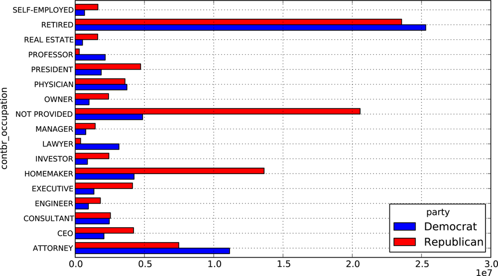
SELF-EMPLOYED 672393.40 1640252.540000It can be easier to look at this data graphically as a bar plot
('barh' means horizontal bar plot,
see Figure 9-2):
In [38]: over_2mm.plot(kind='barh')
You might be interested in the top donor occupations or top
companies donating to Obama and Romney. To do this, you can group by
candidate name and use a variant of the top method from earlier
in the chapter:
def get_top_amounts(group, key, n=5):
    totals = group.groupby(key)['contb_receipt_amt'].sum()

    # Order totals by key in descending order
    return totals.order(ascending=False)[-n:]
Then aggregated by occupation and employer:
In [40]: grouped = fec_mrbo.groupby('cand_nm')

In [41]: grouped.apply(get_top_amounts, 'contbr_occupation', n=7)
Out[41]:
cand_nm        contbr_occupation
Obama, Barack  RETIRED              25305116.38
               ATTORNEY             11141982.97
               NOT PROVIDED          4866973.96
               HOMEMAKER             4248875.80
               PHYSICIAN             3735124.94
               LAWYER                3160478.87
               CONSULTANT            2459912.71
Romney, Mitt   RETIRED              11508473.59
               NOT PROVIDED         11396894.84
               HOMEMAKER             8147446.22
               ATTORNEY              5364718.82
               PRESIDENT             2491244.89
               EXECUTIVE             2300947.03
               C.E.O.                1968386.11
Name: contb_receipt_amt

In [42]: grouped.apply(get_top_amounts, 'contbr_employer', n=10)
Out[42]:
cand_nm        contbr_employer
Obama, Barack  RETIRED               22694358.85
               SELF-EMPLOYED         18626807.16
               NOT EMPLOYED           8586308.70
               NOT PROVIDED           5053480.37
               HOMEMAKER              2605408.54
               STUDENT                 318831.45
               VOLUNTEER               257104.00
               MICROSOFT               215585.36
               SIDLEY AUSTIN LLP       168254.00
               REFUSED                 149516.07
Romney, Mitt   NOT PROVIDED          12059527.24
               RETIRED               11506225.71
               HOMEMAKER              8147196.22
               SELF-EMPLOYED          7414115.22
               STUDENT                 496490.94
               CREDIT SUISSE           281150.00
               MORGAN STANLEY          267266.00
               GOLDMAN SACH & CO.      238250.00
               BARCLAYS CAPITAL        162750.00
               H.I.G. CAPITAL          139500.00
Name: contb_receipt_amtA useful way to analyze this data is to use the cut function to
discretize the contributor amounts into buckets by contribution
size:
In [43]: bins = np.array([0, 1, 10, 100, 1000, 10000, 100000, 1000000, 10000000])

In [44]: labels = pd.cut(fec_mrbo.contb_receipt_amt, bins)

In [45]: labels
Out[45]:
Factor:contb_receipt_amt
array([(10, 100], (100, 1000], (100, 1000], ..., (1, 10], (10, 100],
       (100, 1000]], dtype=object)
Levels (8): array([(0, 1], (1, 10], (10, 100], (100, 1000], (1000, 10000],
       (10000, 100000], (100000, 1000000], (1000000, 10000000]], dtype=object)
We can then group the data for Obama and Romney by name and bin label to get a histogram by donation size:
In [46]: grouped = fec_mrbo.groupby(['cand_nm', labels])

In [47]: grouped.size().unstack(0)
Out[47]:
cand_nm              Obama, Barack  Romney, Mitt
contb_receipt_amt
(0, 1]                         493            77
(1, 10]                      40070          3681
(10, 100]                   372280         31853
(100, 1000]                 153991         43357
(1000, 10000]                22284         26186
(10000, 100000]                  2             1
(100000, 1000000]                3           NaN
(1000000, 10000000]              4           NaN
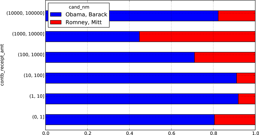
This data shows that Obama has received a significantly larger number of small donations than Romney. You can also sum the contribution amounts and normalize within buckets to visualize percentage of total donations of each size by candidate:
In [48]: bucket_sums = grouped.contb_receipt_amt.sum().unstack(0)

In [49]: bucket_sums
Out[49]:
cand_nm              Obama, Barack  Romney, Mitt
contb_receipt_amt
(0, 1]                      318.24         77.00
(1, 10]                  337267.62      29819.66
(10, 100]              20288981.41    1987783.76
(100, 1000]            54798531.46   22363381.69
(1000, 10000]          51753705.67   63942145.42
(10000, 100000]           59100.00      12700.00
(100000, 1000000]       1490683.08           NaN
(1000000, 10000000]     7148839.76           NaN

In [50]: normed_sums = bucket_sums.div(bucket_sums.sum(axis=1), axis=0)

In [51]: normed_sums
Out[51]:
cand_nm              Obama, Barack  Romney, Mitt
contb_receipt_amt
(0, 1]                    0.805182      0.194818
(1, 10]                   0.918767      0.081233
(10, 100]                 0.910769      0.089231
(100, 1000]               0.710176      0.289824
(1000, 10000]             0.447326      0.552674
(10000, 100000]           0.823120      0.176880
(100000, 1000000]         1.000000           NaN
(1000000, 10000000]       1.000000           NaN

In [52]: normed_sums[:-2].plot(kind='barh', stacked=True)
I excluded the two largest bins as these are not donations by individuals. See Figure 9-3 for the resulting figure.
There are of course many refinements and improvements of this analysis. For example, you could aggregate donations by donor name and zip code to adjust for donors who gave many small amounts versus one or more large donations. I encourage you to download it and explore it yourself.
Aggregating the data by candidate and state is a routine affair:
In [53]: grouped = fec_mrbo.groupby(['cand_nm', 'contbr_st'])

In [54]: totals = grouped.contb_receipt_amt.sum().unstack(0).fillna(0)

In [55]: totals = totals[totals.sum(1) > 100000]

In [56]: totals[:10]
Out[56]:
cand_nm    Obama, Barack  Romney, Mitt
contbr_st
AK             281840.15      86204.24
AL             543123.48     527303.51
AR             359247.28     105556.00
AZ            1506476.98    1888436.23
CA           23824984.24   11237636.60
CO            2132429.49    1506714.12
CT            2068291.26    3499475.45
DC            4373538.80    1025137.50
DE             336669.14      82712.00
FL            7318178.58    8338458.81
If you divide each row by the total contribution amount, you get the relative percentage of total donations by state for each candidate:
In [57]: percent = totals.div(totals.sum(1), axis=0)

In [58]: percent[:10]
Out[58]:
cand_nm    Obama, Barack  Romney, Mitt
contbr_st
AK              0.765778      0.234222
AL              0.507390      0.492610
AR              0.772902      0.227098
AZ              0.443745      0.556255
CA              0.679498      0.320502
CO              0.585970      0.414030
CT              0.371476      0.628524
DC              0.810113      0.189887
DE              0.802776      0.197224
FL              0.467417      0.532583