Chapter 2. Graphs
What’s a Graph?
To most people, a graph is a visual representation of a data set, like a bar chart or an EKG. That’s not what this chapter is about.
In this chapter, a graph is an abstraction used to model a system that contains discrete, interconnected elements. The elements are represented by nodes (also called vertices), and the interconnections are represented by edges.
For example, you could represent a road map with one node for each city and one edge for each road between cities; or you could represent a social network using one node for each person, with an edge between two people if they are “friends” and no edge otherwise.
In some graphs, edges have different lengths (sometimes called “weights” or “costs”). For example, in a road map, the length of an edge might represent the distance between two cities, the travel time, or the bus fare. In a social network, there might be different kinds of edges to represent different kinds of relationships: friends, business associates, and so on.
Edges may be undirected, if they represent a relationship that is symmetric, or directed. In a social network, friendship is usually symmetric: if A is friends with B, then B is friends with A. So you would probably represent friendship with an undirected edge. In a road map, you would probably represent a one-way street with a directed edge.
Graphs have interesting mathematical properties, and there is a branch of mathematics called graph theory that studies them.
Graphs are also useful because there are many real-world problems that can be solved using graph algorithms. For example, Dijkstra’s shortest path algorithm is an efficient way to find the shortest path from a node to all other nodes in a graph. (A path is a sequence of nodes with an edge between each consecutive pair.)
Sometimes the connection between a real-world problem and a graph algorithm is obvious. In the road map example, it is not hard to imagine using a shortest path algorithm to find the route between two cities that minimizes distance (or time, or cost).
In other cases, it takes more effort to represent a problem in a form that can be solved with a graph algorithm and then interpret the solution.
For example, a complex system of radioactive decay can be represented by a graph with one node for each nuclide (type of atom) and an edge between two nuclides if one can decay into the other. A path in this graph represents a decay chain. For more information, see http://en.wikipedia.org/wiki/Radioactive_decay.
The rate of decay between two nuclides is characterized by a decay
constant, ![]() , measured in becquerels (Bq) or decay events per
second. You might be more familiar with half-life,
, measured in becquerels (Bq) or decay events per
second. You might be more familiar with half-life, ![]() , which is the expected time until half of a sample
decays. You can convert from one characterization to the other using the
relation
, which is the expected time until half of a sample
decays. You can convert from one characterization to the other using the
relation ![]() .
.
In our best current model of physics, nuclear decay is a
fundamentally random process, so it is impossible to predict when an
atom will decay. However, given ![]() , the probability that an atom decays during a short
time interval, dt, is
, the probability that an atom decays during a short
time interval, dt, is ![]() .
.
In a graph with multiple decay chains, the probability of a given path is the product of the probabilities of each decay process in the path.
Now suppose you want to find the decay chain with the highest
probability. You could do it by assigning each edge a “length” of
![]() and using a shortest path algorithm.
Why? Because the shortest path algorithm adds up the lengths of the
edges, and adding up log probabilities is the same as multiplying
probabilities. Also, because the logarithms are negated, the smallest
sum corresponds to the largest probability. So the shortest path
corresponds to the most likely decay chain.
and using a shortest path algorithm.
Why? Because the shortest path algorithm adds up the lengths of the
edges, and adding up log probabilities is the same as multiplying
probabilities. Also, because the logarithms are negated, the smallest
sum corresponds to the largest probability. So the shortest path
corresponds to the most likely decay chain.
This is an example of a common and useful process in applying graph algorithms:
Reduce a real-world problem to an instance of a graph problem.
Apply a graph algorithm to compute the result efficiently.
Interpret the result of the computation in terms of a solution to the original problem.
We will see other examples of this process soon.
Read the Wikipedia page about graphs at http://en.wikipedia.org/wiki/Graph_(mathematics) and answer the following questions:
What is a simple graph? In the rest of this section, we will be assuming that all graphs are simple graphs. This is a common assumption for many graph algorithms—so common it is often unstated.
What is a regular graph? What is a complete graph? Prove that a complete graph is regular.
What is a forest? What is a tree? Note: a graph is connected if there is a path from every node to every other node.
Representing Graphs
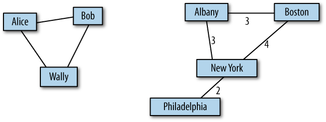
Graphs are usually drawn with squares or circles for nodes and lines for edges. In Figure 2-1, the graph on the left represents a social network with three people.
In the graph on the right, the weights of the edges are the approximate travel times (in hours) between cities in the northeast United States. In this case, the placement of the nodes corresponds roughly to the geography of the cities, but in general the layout of a graph is arbitrary.
To implement graph algorithms, you have to figure out how to represent a graph in the form of a data structure. But to choose the best data structure, you have to know which operations the graph should support.
To get out of this chicken-and-egg problem, I will present a data structure that is a good choice for many graph algorithms. Later we come back and evaluate its pros and cons.
Here is an implementation of a graph as a dictionary of dictionaries:
class Graph(dict):
    def __init__(self, vs=[], es=[]):
        """create a new graph.  (vs) is a list of vertices;
        (es) is a list of edges."""
        for v in vs:
            self.add_vertex(v)

        for e in es:
            self.add_edge(e)

    def add_vertex(self, v):
        """add (v) to the graph"""
        self[v] = {}

    def add_edge(self, e):
        """add (e) to the graph by adding an entry in both directions.

        If there is already an edge connecting these Vertices, the
        new edge replaces it.
        """
        v, w = e
        self[v][w] = e
        self[w][v] = e
The first line declares that Graph inherits from the built-in type dict, so a Graph object has all the methods and operators
of a dictionary.
More specifically, a Graph is a
dictionary that maps from a Vertex
v to an inner dictionary that maps from a Vertex w to an Edge that connects v and
w. So if g is a
graph, g[v][w] maps to an Edge if there is one, and raises a KeyError otherwise.
__init__ takes a
list of vertices and a list of edges as optional parameters. If they are
provided, it calls add_vertex and add_edge to add the vertices and edges to the
graph.
Adding a vertex to a graph means making an entry for it in the
outer dictionary. Adding an edge makes two entries, both pointing to the
same Edge, so this implementation
represents an undirected graph.
Here is the definition for Vertex:
class Vertex(object):
    def __init__(self, label=''):
        self.label = label

    def __repr__(self):
        return 'Vertex(%s)' % repr(self.label)

    __str__ = __repr__
A Vertex is just an object that
has a label attribute. We can add attributes later as needed.
__repr__ is a
special function that returns a string representation of an object. It
is similar to __str__
except that the return value from __str__ is intended to be readable for people,
and the return value from __repr__ is supposed to be a legal Python expression.
The built-in function str
invokes __str__ on an
object; similarly, the built-in function repr invokes __repr__.
In this case, Vertex.__str__ and Vertex.__repr__ refer to the same function, so we
get the same string either way.
Here is the definition for Edge:
class Edge(tuple):
    def __new__(cls, e1, e2):
        return tuple.__new__(cls, (e1, e2))

    def __repr__(self):
        return 'Edge(%s, %s)' % (repr(self[0]), repr(self[1]))

    __str__ = __repr__
Edge inherits from the built-in
type tuple and overrides the __new__ method. When you invoke
an object constructor, Python invokes __new__ to create the object and then __init__ to initialize the
attributes.
For mutable objects, it is most common to override __init__ and use the default
implementation of __new__, but because edges inherit from tuple, they are immutable, which means that
you can’t modify the elements of the tuple in __init__. By overriding __new__, we can use the parameters to initialize
the elements of the tuple.
Here is an example that creates two vertices and an edge:
v = Vertex('v')
    w = Vertex('w')
    e = Edge(v, w)
    print e
Inside Edge.__str__, the term self[0] refers to v and self[1] refers to w, so the output when you print e is:
Edge(Vertex('v'), Vertex('w'))Now we can assemble the edge and vertices into a graph:
g = Graph([v, w], [e])
    print g
The output looks like this (with a little formatting):
{Vertex('w'): {Vertex('v'): Edge(Vertex('v'), Vertex('w'))},
 Vertex('v'): {Vertex('w'): Edge(Vertex('v'), Vertex('w'))}}
We didn’t have to write Graph.__str__; it is inherited from dict.
In this exercise, you will write methods that will be useful for many of the graph algorithms that are coming up.
Download http://thinkcomplex.com/GraphCode.py, which contains the code in this chapter. Run it as a script, and make sure the test code in
maindoes what you expect.Make a copy of
GraphCode.pycalledGraph.py. Add the methods in Steps 3-9 toGraph, adding test code as you go.Write a method named
get_edgethat takes two vertices and returns the edge between them if it exists andNoneotherwise. Hint: use atrystatement.Write a method named
remove_edgethat takes an edge and removes all references to it from the graph.Write a method named
verticesthat returns a list of the vertices in a graph.Write a method named
edgesthat returns a list of edges in a graph. Note that in our representation of an undirected graph, there are two references to each edge.Write a method named
out_verticesthat takes aVertexand returns a list of the adjacent vertices (the ones connected to the given node by an edge).Write a method named
out_edgesthat takes aVertexand returns a list of edges connected to the givenVertex.Write a method named
add_all_edgesthat starts with an edgelessGraphand makes a complete graph by adding edges between all pairs of vertices.
Test your methods by writing test code and checking the output.
Then download http://thinkcomplex.com/GraphWorld.py. GraphWorld is a
simple tool for generating visual representations of graphs. It is
based on the World class in Swampy,
so you might have to install Swampy first: see http://thinkpython.com/swampy.
Read through GraphWorld.py to
get a sense of how it works. Then run it. It should import your
Graph.py and then display a
complete graph with 10 vertices.
Write a method named add_regular_edges that starts with an edgeless
graph and adds edges so that every vertex has the same degree. The
degree of a node is the number of
edges it is connected to.
To create a regular graph with degree 2, you would do something like this:
vertices = [ ... list of Vertices ... ]
g = Graph(vertices, [])
g.add_regular_edges(2)
It is not always possible to create a regular graph with a given degree, so you should figure out and document the preconditions for this method.
To test your code, you might want to create a file named
GraphTest.py that imports Graph.py and GraphWorld.py, then generates and displays
the graphs you want to test.
Random Graphs
A random graph is just what it sounds like: a graph with edges
generated at random. Of course, there are many random processes that can
generate graphs, so there are many kinds of random graphs. One
interesting kind is the Erdős-Rényi model, denoted
![]() , which generates graphs with
n nodes, where the probability is
p that there is an edge between any two nodes. See
http://en.wikipedia.org/wiki/Erdos-Renyi_model.
, which generates graphs with
n nodes, where the probability is
p that there is an edge between any two nodes. See
http://en.wikipedia.org/wiki/Erdos-Renyi_model.
Create a file named RandomGraph.py, and define a class named
RandomGraph that inherits from
Graph and provides a method named
add_random_edges that
takes a probability p as a
parameter and, starting with an edgeless graph, adds edges at random
so that the probability is p that there is an
edge between any two nodes.
Connected Graphs
A graph is connected if there is a path from every node to every other node. See http://en.wikipedia.org/wiki/Connectivity_(graph_theory).
There is a simple algorithm to check whether a graph is connected. Start at any vertex and conduct a search (usually a breadth-first-search or BFS), marking all the vertices you can reach. Then check to see whether all vertices are marked.
You can read about breadth-first-search at http://en.wikipedia.org/wiki/Breadth-first_search.
In general, when you process a node, we say that you are visiting it.
In a search, you visit a node by marking it (so you can tell later that it has been visited), then visiting any unmarked vertices it is connected to.
In a breadth-first-search, you visit nodes in the order they are discovered. You can use a queue or a “worklist” to keep them in order. Here’s how it works:
Start with any vertex and add it to the queue.
Remove a vertex from the queue and mark it. If it is connected to any unmarked vertices, add them to the queue.
If the queue is not empty, go back to Step 2.
Paul Erdős: Peripatetic Mathematician, Speed Freak
Paul Erdős was a Hungarian mathematician who spent most of his career (from 1934 until his death in 1992) living out of a suitcase, visiting colleagues at universities all over the world, and authoring papers with more than 500 collaborators.
He was a notorious caffeine addict and, for the last 20 years of his life, an enthusiastic user of amphetamines. He attributed at least some of his productivity to the use of these drugs; after giving them up for a month to win a bet, he complained that the only result was that mathematics had been set back by a month.[3]
In the 1960s, he and Alfréd Rényi wrote a series of papers introducing the Erdős-Rényi model of random graphs and studying their properties. The second paper is available from http://www.renyi.hu/~p_erdos/1960-10.pdf.
One of their most surprising results is the existence of abrupt changes in the characteristics of random graphs as random edges are added. They showed that for a number of graph properties, there is a threshold value of the probability p below which the property is rare and above which it is almost certain. This transition is sometimes called a “phase change” as an analogy with physical systems that change state at some critical value of temperature. See http://en.wikipedia.org/wiki/Phase_transition.
One of the properties that displays this kind of transition is
connectedness. For a given size n, there is a
critical value, ![]() , such that a random graph
, such that a random graph
![]() is unlikely to be connected if
is unlikely to be connected if
![]() and very likely to be connected if
and very likely to be connected if
![]() .
.
Write a program that tests this result by generating random graphs for values of n and p, and then computing the fraction of the values that are connected.
How does the abruptness of the transition depend on n?
You can download my solution from http://thinkcomplex.com/RandomGraph.py.
Iterators
If you have read the documentation of Python dictionaries, you
might have noticed the methods iterkeys, itervalues, and iteritems. These methods are similar to
keys, values, and items except that instead of building a new
list, they return iterators.
An iterator is an object that
provides a method named next that
returns the next element in a sequence. Here is an example that creates
a dictionary and uses iterkeys to
traverse the keys.
>>> d = dict(a=1, b=2)
>>> iter = d.iterkeys()
>>> print iter.next()
a
>>> print iter.next()
b
>>> print iter.next()
Traceback (most recent call last):
  File "<stdin>", line 1, in <module>
StopIteration
The first time next is invoked,
it returns the first key from the dictionary (the order of the keys is
arbitrary). The second time it is invoked, it returns the second
element. The third time, and every time thereafter, it raises a StopIteration exception.
An iterator can be used in a for loop; for example, the following is a
common idiom for traversing the key-value pairs in a
dictionary:
for k, v in d.iteritems():
        print k, v
In this context, iteritems is
likely to be faster than items
because it doesn’t have to build the entire list of tuples; it reads
them from the dictionary as it goes along.
But it is only safe to use the iterator methods if you do not add or remove dictionary keys inside the loop. Otherwise you get an exception:
>>> d = dict(a=1)
>>> for k in d.iterkeys():
...     d['b'] = 2
...
RuntimeError: dictionary changed size during iteration
Another limitation of iterators is that they do not support index operations:
>>> iter = d.iterkeys()
>>> print iter[1]
TypeError: 'dictionary-keyiterator' object is unsubscriptable
If you need indexed access, you should use keys. Alternatively, the Python module
itertools provides many useful
iterator functions.
A user-defined object can be used as an iterator if it provides
methods named next and __iter__. The following example
is an iterator that always returns True:
class AllTrue(object):
    def next(self):
        return True

    def __iter__(self):
        return self
The __iter__
method for iterators returns the iterator itself. This protocol makes it
possible to use iterators and sequences interchangeably in many
contexts.
Iterators like AllTrue can
represent an infinite sequence. They are useful as an argument to
zip:
>>> print zip('abc', AllTrue())
[('a', True), ('b', True), ('c', True)]
Generators
For many purposes, the easiest way to make an iterator is to write
a generator, which is a function that
contains a yield statement. yield is similar to return, except that the state of the running
function is stored and can be resumed.
For example, here is a generator that yields successive letters of the alphabet:
def generate_letters():
    for letter in 'abc':
        yield letter
When you call this function, the return value is an iterator:
>>> iter = generate_letters()
>>> print iter
<generator object at 0xb7d4ce4c>
>>> print iter.next()
a
>>> print iter.next()
b
And you can use an iterator in a for loop:
>>> for letter in generate_letters():
...     print letter
...
a
b
c
A generator with an infinite loop returns an iterator that never terminates. For example, here’s a generator that cycles through the letters of the alphabet:
def alphabet_cycle():
    while True:
        for c in string.lowercase:
            yield c