
Chapter 3. Analysis of Algorithms
Analysis of algorithms is the branch of computer science that studies the performance of algorithms, especially their runtime and space requirements. For more information, see http://en.wikipedia.org/wiki/Analysis_of_algorithms.
The practical goal of algorithm analysis is to predict the performance of different algorithms in order to guide design decisions.
During the 2008 United States presidential campaign, candidate Barack Obama was asked to perform an impromptu analysis when he visited Google. Chief executive Eric Schmidt jokingly asked him for “the most efficient way to sort a million 32-bit integers.” Obama had apparently been tipped off, because he quickly replied, “I think the bubble sort would be the wrong way to go.” See http://www.youtube.com/watch?v=k4RRi_ntQc8.
This is true: bubble sort is conceptually simple but slow for large datasets. The answer Schmidt was probably looking for is “radix sort” (see http://en.wikipedia.org/wiki/Radix_sort).[4]
The goal of algorithm analysis is to make meaningful comparisons between algorithms, but there are some problems:
The relative performance of the algorithms might depend on characteristics of the hardware, so one algorithm might be faster on Machine A, another on Machine B. The general solution to this problem is to specify a machine model and analyze the number of steps (or operations) an algorithm requires under a given model.
Relative performance might depend on the details of the dataset. For example, some sorting algorithms run faster if the data are already partially sorted; other algorithms run slower in this case. A common way to avoid this problem is to analyze the worst case scenario. It is also sometimes useful to analyze average case performance, but it is usually harder, and sometimes it is not clear what set of cases to average.
Relative performance also depends on the size of the problem. A sorting algorithm that is fast for small lists might be slow for long lists. The usual solution to this problem is to express runtime (or number of operations) as a function of problem size and to compare the functions asymptotically as the problem size increases.
The good thing about this kind of comparison is that it lends itself
to simple classification of algorithms. For example, if I know that the
runtime of Algorithm A tends to be proportional to the size of the input
n, and Algorithm B tends to be proportional to
![]() , then I expect A to be faster than B for large values
of n.
, then I expect A to be faster than B for large values
of n.
This kind of analysis comes with some caveats, but we’ll get to that later.
Order of Growth
Suppose you have analyzed two algorithms and expressed their
runtimes in terms of the size of the input: Algorithm A takes
![]() steps to solve a problem with size
n, and Algorithm B takes
steps to solve a problem with size
n, and Algorithm B takes ![]() steps.
steps.
The following table shows the runtime of these algorithms for different problem sizes:
| Input size | Runtime of Algorithm A | Runtime of Algorithm B |
| 10 | 1 001 | 111 |
| 100 | 10 001 | 10 101 |
| 1 000 | 100 001 | 1 001 001 |
| 10 000 | 1 000 001 |
At ![]() , Algorithm A looks pretty bad; it takes almost 10
times longer than Algorithm B. But for
, Algorithm A looks pretty bad; it takes almost 10
times longer than Algorithm B. But for ![]() , they are about the same, and for larger values, A
is much better.
, they are about the same, and for larger values, A
is much better.
The fundamental reason is that for large values of
n, any function that contains an ![]() term will grow faster than a function whose leading
term is n. The leading
term is the term with the highest exponent.
term will grow faster than a function whose leading
term is n. The leading
term is the term with the highest exponent.
For Algorithm A, the leading term has a large coefficient, 100,
which is why B does better than A for a small n.
But regardless of the coefficients, there will always be some value of
n where ![]() .
.
The same argument applies to the non-leading terms. Even if the
runtime of Algorithm A were ![]() , it would still be better than Algorithm B for a
sufficiently large n.
, it would still be better than Algorithm B for a
sufficiently large n.
In general, we expect an algorithm with a smaller leading term to be a better algorithm for large problems, but for smaller problems, there may be a crossover point where another algorithm is better. The location of the crossover point depends on the details of the algorithms, the inputs, and the hardware, so it is usually ignored for purposes of algorithmic analysis. But that doesn’t mean you can forget about it.
If two algorithms have the same leading order term, it is hard to say which is better; again, the answer depends on the details. So for algorithmic analysis, functions with the same leading term are considered equivalent, even if they have different coefficients.
An order of growth is a set of
functions whose asymptotic growth behavior is considered equivalent. For
example, 2n, 100n, and
![]() belong to the same order of growth, which is written
belong to the same order of growth, which is written
![]() in Big O
notation, and often called linear because every function in the set grows
linearly with n.
in Big O
notation, and often called linear because every function in the set grows
linearly with n.
All functions with the leading term ![]() belong to
belong to ![]() ; they are quadratic, which is a fancy word for functions
with the leading term
; they are quadratic, which is a fancy word for functions
with the leading term ![]() .
.
The following table shows some of the orders of growth that appear most commonly in algorithmic analysis, in increasing order of badness.
| Order of growth | Name |
| constant | |
| logarithmic (for any b) | |
| linear | |
| “en log en” | |
| quadratic | |
| cubic | |
| exponential (for any c) |
For the logarithmic terms, the base of the logarithm doesn’t matter; changing bases is the equivalent of multiplying by a constant, which doesn’t change the order of growth. Similarly, all exponential functions belong to the same order of growth regardless of the base of the exponent. Exponential functions grow very quickly, so exponential algorithms are only useful for small problems.
Read the Wikipedia page on Big O notation at http://en.wikipedia.org/wiki/Big_O_notation, and answer the following questions:
Programmers who care about performance often find this kind of analysis hard to swallow. They have a point: sometimes the coefficients and the non-leading terms make a real difference, and sometimes the details of the hardware, the programming language, and the characteristics of the input make a big difference. Also, for small problems, asymptotic behavior is irrelevant.
But if you keep those caveats in mind, algorithmic analysis is a useful tool. At least for large problems, the “better” algorithm is usually better, and sometimes it is much better. The difference between two algorithms with the same order of growth is usually a constant factor, but the difference between a good algorithm and a bad algorithm is unbounded!
Analysis of Basic Python Operations
Most arithmetic operations are constant time; multiplication usually takes longer than addition and subtraction, and division takes even longer, but these runtimes don’t depend on the magnitude of the operands. Very large integers are an exception; in that case, the runtime increases with the number of digits.
Indexing operations—reading or writing elements in a sequence or dictionary—are also constant time, regardless of the size of the data structure.
A for loop that traverses a
sequence or dictionary is usually linear, as long as all of the
operations in the body of the loop are constant time. For example,
adding up the elements of a list is linear:
total = 0
    for x in t:
        total += x
The built-in function sum is
also linear because it does the same thing, but it tends to be faster
because it is a more efficient implementation. In the language of
algorithmic analysis, it has a smaller leading coefficient.
If you use the same loop to “add” a list of strings, the runtime
is quadratic because string concatenation is linear. The string method join
is usually faster because it is linear in the total length of the
strings.
As a rule of thumb, if the body of a loop is in ![]() , then the whole loop is in
, then the whole loop is in ![]() . The exception is if you can show that the loop
exits after a constant number of iterations. If a loop runs
k times regardless of n, then
the loop is in
. The exception is if you can show that the loop
exits after a constant number of iterations. If a loop runs
k times regardless of n, then
the loop is in ![]() , even for a large k.
, even for a large k.
Multiplying by k doesn’t change the order of
growth, but neither does dividing. So if the body of a loop is in
![]() and it runs
and it runs ![]() times, the loop is in
times, the loop is in ![]() , even for a large k.
, even for a large k.
Most string and tuple operations are linear, except indexing and
len, which are constant time. The
built-in functions min and max are linear. The runtime of a slice
operation is proportional to the length of the output, but independent
of the size of the input.
All string methods are linear, but if the lengths of the strings are bounded by a constant—for example, operations on single characters—they are considered constant time.
Most list methods are linear, but there are some exceptions:
Adding an element to the end of a list is constant time on average. When it runs out of room, it occasionally gets copied to a bigger location, but the total time for n operations is
 , so we say that the “amortized”
time for one operation is
, so we say that the “amortized”
time for one operation is  .
.Removing an element from the end of a list is constant time.
Most dictionary operations and methods are constant time, but there are some exceptions:
The runtime of
copyis proportional to the number of elements, but not to the size of the elements (it copies references, not the elements themselves).The runtime of
updateis proportional to the size of the dictionary passed as a parameter, not the dictionary being updated.keys,values, anditemsare linear because they return new lists;iterkeys,itervalues, anditeritemsare constant time because they return iterators. But if you loop through the iterators, the loop will be linear. Using the “iter” functions saves some overhead, but it doesn’t change the order of growth unless the number of items you access is bounded.
The performance of dictionaries is one of the minor miracles of computer science. We will see how they work in Hashtables.
Read the Wikipedia page on sorting algorithms at http://en.wikipedia.org/wiki/Sorting_algorithm, and answer the following questions:
What is a “comparison sort”? What is the best worst-case order of growth for a comparison sort? What is the best worst-case order of growth for any sort algorithm?
What is the order of growth of bubble sort, and why does Barack Obama think it is “the wrong way to go”?
What is the order of growth of radix sort? What preconditions do we need to use it?
What is the worst sorting algorithm (that has a name)?
What sort algorithm does the C library use? What sort algorithm does Python use? Are these algorithms stable? (You might have to Google around to find these answers.)
Many of the non-comparison sorts are linear, so why does Python use an
 comparison sort?
Analysis of Search Algorithms
A search is an algorithm that takes a collection and a target item and determines whether the target is in the collection, often returning the index of the target.
The simplest search algorithm is a “linear search,” which traverses the items of the collection in order, stopping if it finds the target. In the worst case, it has to traverse the entire collection, so the runtime is linear.
The in operator for sequences
uses a linear search; so do string methods like find and count.
If the elements of the sequence are in order, you can use a
bisection search, which is
![]() . Bisection search is similar to the
algorithm you probably use to look a word up in a dictionary (a real
dictionary, not the data structure). Instead of starting at the
beginning and checking each item in order, you start with the item in
the middle and check whether the word you are looking for comes before
or after. If it comes before, then you search the first half of the
sequence. Otherwise, you search the second half. Either way, you cut the
number of remaining items in half.
. Bisection search is similar to the
algorithm you probably use to look a word up in a dictionary (a real
dictionary, not the data structure). Instead of starting at the
beginning and checking each item in order, you start with the item in
the middle and check whether the word you are looking for comes before
or after. If it comes before, then you search the first half of the
sequence. Otherwise, you search the second half. Either way, you cut the
number of remaining items in half.
If the sequence has 1,000,000 items, it will take about 20 steps to find the word or conclude that it’s not there. So that’s about 50,000 times faster than a linear search.
Bisection search can be much faster than linear search, but it requires the sequence to be in order, which might require extra work.
There is another data structure called a hashtable that is even faster—it can do a search
in constant time, and doesn’t require the items to be sorted. Python
dictionaries are implemented using hashtables, which is why most
dictionary operations, including the in operator, are constant time.
Hashtables
To explain how hashtables work and why their performance is so good, I start with a simple implementation of a map and gradually improve it until it’s a hashtable.
I use Python to demonstrate these implementations, but in real life you wouldn’t write code like this in Python; you would just use a dictionary! So for the rest of this chapter, you have to imagine that dictionaries don’t exist and you want to implement a data structure that maps from keys to values. The operations you have to implement are:
add(k, v):Add a new item that maps from key
kto valuev. With a Python dictionary,d, this operation is writtend[k] = v.get(target):Look up and return the value that corresponds to key
target. With a Python dictionary,d, this operation is writtend[target]ord.get(target).
For now, I assume that each key only appears once. The simplest implementation of this interface uses a list of tuples, where each tuple is a key-value pair:
class LinearMap(object):

    def __init__(self):
        self.items = []

    def add(self, k, v):
        self.items.append((k, v))

    def get(self, k):
        for key, val in self.items:
            if key == k:
                return val
        raise KeyError
add appends a key-value tuple
to the list of items, which takes constant time.
get uses a for loop to search the list. If it finds the
target key, it returns the corresponding value; otherwise, it raises a
KeyError (so get is linear).
An alternative is to keep the list sorted by key. Then get could use a bisection search, which is
![]() . But inserting a new item in the
middle of a list is linear, so this might not be the best option. There
are other data structures (see http://en.wikipedia.org/wiki/Red-black_tree) that can
implement
. But inserting a new item in the
middle of a list is linear, so this might not be the best option. There
are other data structures (see http://en.wikipedia.org/wiki/Red-black_tree) that can
implement add and get in log time, but that’s still not as good
as constant time, so let’s move on.
One way to improve LinearMap is
to break the list of key-value pairs into smaller lists. Here’s an
implementation called BetterMap,
which is a list of 100 LinearMaps. As
we’ll see in a second, the order of growth for get is still linear, but BetterMap is a step on the path toward
hashtables:
class BetterMap(object):

    def __init__(self, n=100):
        self.maps = []
        for i in range(n):
            self.maps.append(LinearMap())

    def find_map(self, k):
        index = hash(k) % len(self.maps)
        return self.maps[index]

    def add(self, k, v):
        m = self.find_map(k)
        m.add(k, v)

    def get(self, k):
        m = self.find_map(k)
        return m.get(k)
__init__ makes a
list of n LinearMaps.
find_map is used
by add and get to figure out which map to put the new
item in, or which map to search.
find_map uses the
built-in function hash, which takes
almost any Python object and returns an integer. A limitation of this
implementation is that it only works with hashable keys. Mutable types
like lists and dictionaries are unhashable.
Hashable objects that are considered equal return the same hash value, but the converse is not necessarily true: two different objects can return the same hash value.
find_map uses the
modulus operator to wrap the hash values into the range from 0 to
len(self.maps), so the result is a
legal index into the list. Of course, this means that many different
hash values will wrap onto the same index. But if the hash function
spreads things out pretty evenly (which is what hash functions are
designed to do), then we expect ![]() items per
items per LinearMap.
Since the runtime of LinearMap.get is proportional to the number of
items, we expect BetterMap to be
about 100 times faster than LinearMap. The order of growth is still
linear, but the leading coefficient is smaller. That’s nice, but still
not as good as a hashtable.
Here (finally) is the crucial idea that makes hashtables fast: if
you can keep the maximum length of the LinearMaps bounded, LinearMap.get is constant time. All you have
to do is keep track of the number of items, and when the number of items
per LinearMap exceeds a threshold,
resize the hashtable by adding more LinearMaps.
Here is an implementation of a hashtable:
class HashMap(object):

    def __init__(self):
        self.maps = BetterMap(2)
        self.num = 0

    def get(self, k):
        return self.maps.get(k)

    def add(self, k, v):
        if self.num == len(self.maps.maps):
            self.resize()

        self.maps.add(k, v)
        self.num += 1

    def resize(self):
        new_maps = BetterMap(self.num * 2)

        for m in self.maps.maps:
            for k, v in m.items:
                new_maps.add(k, v)

        self.maps = new_maps
Each HashMap contains a
BetterMap. __init__ starts with just two LinearMaps and initializes num, which keeps track of the number of
items.
get just dispatches to BetterMap. The real work happens in add, which checks the number of items and the
size of the BetterMap: if they are
equal, the average number of items per LinearMap is 1, so it calls resize.
resize makes a new BetterMap, twice as big as the previous one,
and then “rehashes” the items from the old map to the new.
Rehashing is necessary because changing the number of LinearMaps changes the denominator of the
modulus operator in find_map. That means that some objects that used
to wrap into the same LinearMap will
get split up—which is what we wanted, right?
Rehashing is linear, so resize
is linear, which might seem bad since I promised that add would be constant time. But remember that
we don’t have to resize every time, so add is usually constant time and only
occasionally linear. The total amount of work to run add n times is
proportional to n, so the average time of each
add is constant time!
To see how this works, think about starting with an empty
hashtable and adding a sequence of items. We start with two LinearMaps, so the first two adds are fast (no resizing required). Let’s
say that they take one unit of work each. The next add requires a resize, so we have to rehash
the first two items (let’s call that two more units of work) and then
add the third item (one more unit). Adding the next item costs one unit,
so the total so far is six units of work for four items.
The next add costs 5 units, but
the next three are only 1 unit each, so the total is 14 units for the
first 8 adds.
The next add costs 9 units, but
then we can add 7 more before the next resize, so the total is 30 units
for the first 16 adds.
After 32 adds, the total cost
is 62 units, and I hope you are starting to see a pattern. After
n adds, where
n is a power of two, the total cost is
![]() units, so the average work per
units, so the average work per add is a little less than two units. When
n is a power of two, that’s the best case; for
other values of n, the average work is a little
higher, but that’s not important. The important thing is that it is
![]() .
.
Figure 3-1 shows how this works graphically. Each
block represents a unit of work. The columns show the total work for
each add in order from left to right; the first two adds cost one unit, the third costs three
units, etc.
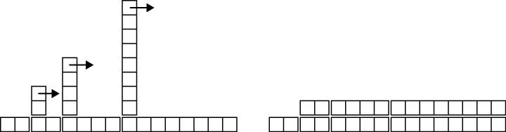
The extra work of rehashing appears as a sequence of increasingly
tall towers with increasing space between them. Now if you knock over
the towers, amortizing the cost of resizing over all adds, you can see graphically that the total
cost after n adds is ![]() .
.
An important feature of this algorithm is that when we resize the
hashtable, it grows geometrically; that is, we multiply the size by a
constant. If you increase the size arithmetically—adding a fixed number
each time—the average time per add is
linear.
You can download my implementation of HashMap from http://thinkcomplex.com/Map.py, but remember that there is no reason to use it; if you want a map, just use a Python dictionary.
A drawback of hashtables is that the elements have to be hashable, which usually means they have to be immutable. That’s why, in Python, you can use tuples but not lists as keys in a dictionary. An alternative is to use a tree-based map.
Write an implementation of the map interface called TreeMap that uses a red-black tree to
perform add and get in log time.
Summing Lists
Suppose you have a bunch of lists and you want to join them up into a single list. There are three ways you might do that in Python.
Without knowing how +=,
extend, and sum are implemented, it is hard to analyze
their performance. For example, if total +=
x creates a new list every time, the loop is quadratic, but if
it modifies total, it’s
linear.
To find out, we could read the source code, but as an exercise, let’s see if we can figure it out by measuring runtimes.
A simple way to measure the runtime of a program is to use the
function times in the os module, which returns a tuple of floats
indicating the time your process has used (see the documentation for
details). I use a function, etime,
which returns the sum of “user time” and “system time” (which is usually
what we care about for performance measurement):
import os

def etime():
    """See how much user and system time this process has used
    so far and return the sum."""

    user, sys, chuser, chsys, real = os.times()
    return user+sys
To measure the elapsed time of a function, you can call etime twice and compute the difference:
start = etime()

    # put the code you want to measure here

    end = etime()
    elapsed = end - start
Alternatively, if you use IPython, you can use the timeit command. See http://ipython.scipy.org.
If an algorithm is quadratic, we expect the runtime, t, as a function of input size, n, to look like this:
where a, b, and c are unknown coefficients. If you take the log of both sides, you get:
For large values of n, the non-leading terms are insignificant and this approximation is pretty good. So if we plot t versus n on a log-log scale, we expect a straight line with slope 2.
Similarly, if the algorithm is linear, we expect a line with slope 1.
I wrote three functions that concatenate lists: sum_plus uses +=, sum_extend uses list.extend, and sum_sum uses sum. I timed them for a range of n and plotted the results on a log-log scale.
Figures 3-2 and
3-3 show the
results.
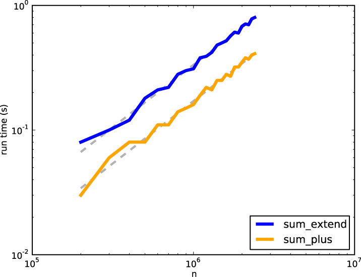

In Figure 3-2, I fit a line with slope 1 to the
curves. The data fit this line well, so we conclude that these
implementations are linear. The implementation for += is faster by a constant factor because it
takes some time to look up the extend
method each time through the loop.
In Figure 3-3, the data fit a line with slope 2,
so the implementation of sum is
quadratic.
pyplot
To make the figures in this section, I used pyplot, which is part of matplotlib. If matplotlib is not part of your Python
installation, you might have to install it, or you can use another
library to make plots.
Here’s an example that makes a simple plot:
import matplotlib.pyplot as pyplot

pyplot.plot(xs, ys)
scale = 'log'
pyplot.xscale(scale)
pyplot.yscale(scale)
pyplot.title('')
pyplot.xlabel('n')
pyplot.ylabel('run time (s)')
pyplot.show()
The import statement makes matplotlib.pyplot accessible with the shorter
name pyplot.
plot takes a list of
x-values and a list of
y-values and plots them. The lists have to have the
same length. xscale and yscale make the axes either linear or
logarithmic.
title, xlabel, and ylabel are self-explanatory. Finally, show displays the plot on the screen. You
could also use savefig to save the
plot in a file.
Documentation of pyplot is
available at http://matplotlib.sourceforge.net/.
Test the performance of LinearMap, BetterMap, and HashMap; see if you can characterize their
order of growth.
You can download my map implementations from http://thinkcomplex.com/Map.py and the code I used in this section from http://thinkcomplex.com/listsum.py.
You will have to find a range of n that is big enough to show asymptotic
behavior, but small enough to run quickly.
List Comprehensions
One of the most common programming patterns is to traverse a list while building a new list.
Here is an example that computes the square of each element in a list and accumulates the results:
res = []
    for x in t:
        res.append(x**2)
This pattern is so common that Python provides a more concise syntax for it, called a list comprehension. In this context, the sense of “comprehend” is something like “contain” rather than “understand.” See http://en.wikipedia.org/wiki/List_comprehension. Here’s what it looks like:
res = [x**2 for x in t]
This expression yields the same result as the previous loop. List comprehensions tend to be fast because the loop is executed in C rather than Python. The drawback is that they are harder to debug.
List comprehensions can include an if clause that selects a subset of the items.
The following example makes a list of the positive elements in t:
res = [x for x in t if x > 0]
The following is a common idiom for making a list of tuples, where each tuple is a value and a key from a dictionary:
res = [(v, k) for k, v in d.iteritems()]
In this case, it is safe to use iteritems rather than items because the loop does not modify the
dictionary. Also, it is likely to be faster because it doesn’t have to
make a list, just an iterator.
It is also possible to nest for
loops inside a list comprehension. The following example builds a list
of Edges between each pair of
vertices in vs:
edges = [Edge(v, w) for v in vs for w in vs if v is not w]
That’s pretty concise, but complicated comprehensions can be hard to read, so use them sparingly.
[4] But if you get a question like this in an interview, I think a better answer is, “The fastest way to sort a million integers is to use whatever sort function is provided by the language I’m using. Its performance is good enough for the vast majority of applications, but if it turned out that my application was too slow, I would use a profiler to see where the time was being spent. If it looked like a faster sort algorithm would have a significant effect on performance, then I would look around for a good implementation of radix sort.”