Chapter 43. Designing for Scale
Elasticsearch is used by some companies to index and search petabytes of data every day, but most of us start out with something a little more humble in size. Even if we aspire to be the next Facebook, it is unlikely that our bank balance matches our aspirations. We need to build for what we have today, but in a way that will allow us to scale out flexibly and rapidly.
Elasticsearch is built to scale. It will run very happily on your laptop or in a cluster containing hundreds of nodes, and the experience is almost identical. Growing from a small cluster to a large cluster is almost entirely automatic and painless. Growing from a large cluster to a very large cluster requires a bit more planning and design, but it is still relatively painless.
Of course, it is not magic. Elasticsearch has its limitations too. If you are aware of those limitations and work with them, the growing process will be pleasant. If you treat Elasticsearch badly, you could be in for a world of pain.
The default settings in Elasticsearch will take you a long way, but to get the most bang for your buck, you need to think about how data flows through your system. We will talk about two common data flows: time-based data (such as log events or social network streams, where relevance is driven by recency), and user-based data (where a large document collection can be subdivided by user or customer).
This chapter will help you make the right decisions up front, to avoid nasty surprises later.
The Unit of Scale
In “Dynamically Updatable Indices”, we explained that a shard is a Lucene index and that an Elasticsearch index is a collection of shards. Your application talks to an index, and Elasticsearch routes your requests to the appropriate shards.
A shard is the unit of scale. The smallest index you can have is one with a single shard. This may be more than sufficient for your needs—a single shard can hold a lot of data—but it limits your ability to scale.
Imagine that our cluster consists of one node, and in our cluster we have one index, which has only one shard:
PUT/my_index{"settings":{"number_of_shards":1,
"number_of_replicas":0}}
Create an index with one primary shard and zero replica shards.
This setup may be small, but it serves our current needs and is cheap to run.
Note
At the moment we are talking about only primary shards. We discuss replica shards in “Replica Shards”.
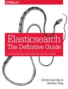
One glorious day, the Internet discovers us, and a single node just can’t keep up with the traffic. We decide to add a second node, as per Figure 43-1. What happens?

Figure 43-1. An index with one shard has no scale factor
The answer is: nothing. Because we have only one shard, there is nothing to put on the second node. We can’t increase the number of shards in the index, because the number of shards is an important element in the algorithm used to route documents to shards:
shard = hash(routing) % number_of_primary_shards
Our only option now is to reindex our data into a new, bigger index that has more shards, but that will take time that we can ill afford. By planning ahead, we could have avoided this problem completely by overallocating.
Shard Overallocation
A shard lives on a single node, but a node can hold multiple shards. Imagine that we created our index with two primary shards instead of one:
PUT/my_index{"settings":{"number_of_shards":2,"number_of_replicas":0}}
Create an index with two primary shards and zero replica shards.
With a single node, both shards would be assigned to the same node. From the point of view of our application, everything functions as it did before. The application communicates with the index, not the shards, and there is still only one index.
This time, when we add a second node, Elasticsearch will automatically move one shard from the first node to the second node, as depicted in Figure 43-2. Once the relocation has finished, each shard will have access to twice the computing power that it had before.
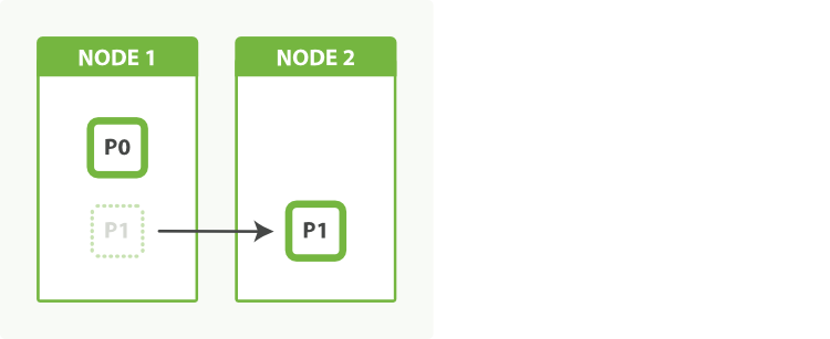
Figure 43-2. An index with two shards can take advantage of a second node
We have been able to double our capacity by simply copying a shard across the network to the new node. The best part is, we achieved this with zero downtime. All indexing and search requests continued to function normally while the shard was being moved.
A new index in Elasticsearch is allotted five primary shards by default. That means that we can spread that index out over a maximum of five nodes, with one shard on each node. That’s a lot of capacity, and it happens without you having to think about it at all!
Kagillion Shards
The first thing that new users do when they learn about shard overallocation is to say to themselves:
I don’t know how big this is going to be, and I can’t change the index size later on, so to be on the safe side, I’ll just give this index 1,000 shards…
A new user
One thousand shards—really? And you don’t think that, perhaps, between now and the time you need to buy one thousand nodes, that you may need to rethink your data model once or twice and have to reindex?
A shard is not free. Remember:
-
A shard is a Lucene index under the covers, which uses file handles, memory, and CPU cycles.
-
Every search request needs to hit a copy of every shard in the index. That’s fine if every shard is sitting on a different node, but not if many shards have to compete for the same resources.
-
Term statistics, used to calculate relevance, are per shard. Having a small amount of data in many shards leads to poor relevance.
Tip
A little overallocation is good. A kagillion shards is bad. It is difficult to define what constitutes too many shards, as it depends on their size and how they are being used. A hundred shards that are seldom used may be fine, while two shards experiencing very heavy usage could be too many. Monitor your nodes to ensure that they have enough spare capacity to deal with exceptional conditions.
Scaling out should be done in phases. Build in enough capacity to get to the next phase. Once you get to the next phase, you have time to think about the changes you need to make to reach the phase after that.
Capacity Planning
If 1 shard is too few and 1,000 shards are too many, how do I know how many shards I need? This is a question that is impossible to answer in the general case. There are just too many variables: the hardware that you use, the size and complexity of your documents, how you index and analyze those documents, the types of queries that you run, the aggregations that you perform, how you model your data, and more.
Fortunately, it is an easy question to answer in the specific case—yours:
-
Create a cluster consisting of a single server, with the hardware that you are considering using in production.
-
Create an index with the same settings and analyzers that you plan to use in production, but with only one primary shard and no replicas.
-
Fill it with real documents (or as close to real as you can get).
-
Run real queries and aggregations (or as close to real as you can get).
Essentially, you want to replicate real-world usage and to push this single shard until it “breaks.” Even the definition of breaks depends on you: some users require that all responses return within 50ms; others are quite happy to wait for 5 seconds.
Once you define the capacity of a single shard, it is easy to extrapolate that number to your whole index. Take the total amount of data that you need to index, plus some extra for future growth, and divide by the capacity of a single shard. The result is the number of primary shards that you will need.
Tip
Capacity planning should not be your first step.
First look for ways to optimize how you are using Elasticsearch. Perhaps you have inefficient queries, not enough RAM, or you have left swap enabled?
We have seen new users who, frustrated by initial performance, immediately start trying to tune the garbage collector or adjust the number of threads, instead of tackling the simple problems like removing wildcard queries.
Replica Shards
Up until now we have spoken only about primary shards, but we have another tool in our belt: replica shards. The main purpose of replicas is for failover, as discussed in Chapter 2: if the node holding a primary shard dies, a replica is promoted to the role of primary.
At index time, a replica shard does the same amount of work as the primary shard. New documents are first indexed on the primary and then on any replicas. Increasing the number of replicas does not change the capacity of the index.
However, replica shards can serve read requests. If, as is often the case, your index is search heavy, you can increase search performance by increasing the number of replicas, but only if you also add extra hardware.
Let’s return to our example of an index with two primary shards. We increased capacity of the index by adding a second node. Adding more nodes would not help us to add indexing capacity, but we could take advantage of the extra hardware at search time by increasing the number of replicas:
POST/my_index/_settings{"number_of_replicas":1}
Having two primary shards, plus a replica of each primary, would give us a total of four shards: one for each node, as shown in Figure 43-3.
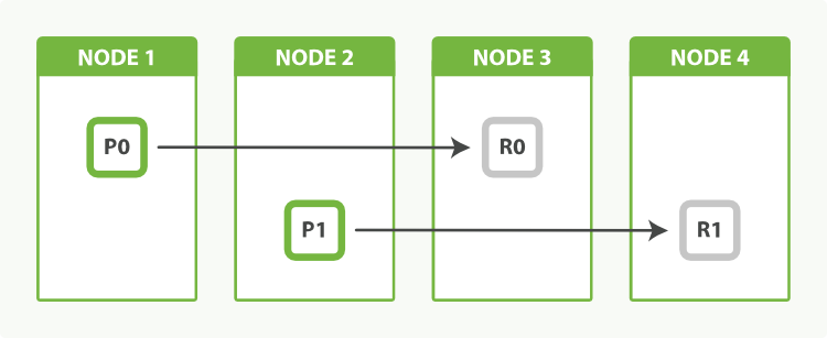
Figure 43-3. An index with two primary shards and one replica can scale out across four nodes
Balancing Load with Replicas
Search performance depends on the response times of the slowest node, so it is a good idea to try to balance out the load across all nodes. If we added just one extra node instead of two, we would end up with two nodes having one shard each, and one node doing double the work with two shards.
We can even things out by adjusting the number of replicas. By allocating two replicas instead of one, we end up with a total of six shards, which can be evenly divided between three nodes, as shown in Figure 43-4:
POST/my_index/_settings{"number_of_replicas":2}
As a bonus, we have also increased our availability. We can now afford to lose two nodes and still have a copy of all our data.
Figure 43-4. Adjust the number of replicas to balance the load between nodes
Note
The fact that node 3 holds two replicas and no primaries is not important. Replicas and primaries do the same amount of work; they just play slightly different roles. There is no need to ensure that primaries are distributed evenly across all nodes.Multiple Indices
Finally, remember that there is no rule that limits your application to using only a single index. When we issue a search request, it is forwarded to a copy (a primary or a replica) of all the shards in an index. If we issue the same search request on multiple indices, the exact same thing happens—there are just more shards involved.
Tip
Searching 1 index of 50 shards is exactly equivalent to searching 50 indices with 1 shard each: both search requests hit 50 shards.This can be a useful fact to remember when you need to add capacity on the fly. Instead of having to reindex your data into a bigger index, you can just do the following:
-
Create a new index to hold new data.
-
Search across both indices to retrieve new and old data.
In fact, with a little forethought, adding a new index can be done in a completely transparent way, without your application ever knowing that anything has changed.
In “Index Aliases and Zero Downtime”, we spoke about using an index alias to point to the
current version of your index. For instance, instead of naming your index
tweets, name it tweets_v1. Your application would still talk to tweets,
but in reality that would be an alias that points to tweets_v1. This allows
you to switch the alias to point to a newer version of the index on the fly.
A similar technique can be used to expand capacity by adding a new index. It requires a bit of planning because you will need two aliases: one for searching and one for indexing:
PUT/tweets_1/_alias/tweets_searchPUT/tweets_1/_alias/tweets_index
Both the
tweets_searchand thetweets_indexalias point to indextweets_1.
New documents should be indexed into tweets_index, and searches should be
performed against tweets_search. For the moment, these two aliases point to
the same index.
When we need extra capacity, we can create a new index called tweets_2 and
update the aliases as follows:
POST/_aliases{"actions":[{"add":{"index":"tweets_2","alias":"tweets_search"}},{"remove":{"index":"tweets_1","alias":"tweets_index"}},
{"add":{"index":"tweets_2","alias":"tweets_index"}}]}
Add index
tweets_2to thetweets_searchalias.Switch
tweets_indexfromtweets_1totweets_2.
A search request can target multiple indices, so having the search alias point
to tweets_1 and tweets_2 is perfectly valid. However, indexing requests can
target only a single index. For this reason, we have to switch the index alias
to point to only the new index.
Tip
A document GET request, like an indexing request, can target only one index.
This makes retrieving a document by ID a bit more complicated in this
scenario. Instead, run a search request with the
ids query, or do a
multi-get request on tweets_1 and tweets_2.
Using multiple indices to expand index capacity on the fly is of particular benefit when dealing with time-based data such as logs or social-event streams, which we discuss in the next section.
Time-Based Data
One of the most common use cases for Elasticsearch is for logging, so common in fact that Elasticsearch provides an integrated logging platform called the ELK stack—Elasticsearch, Logstash, and Kibana—to make the process easy.
Logstash collects, parses, and enriches logs before indexing them into Elasticsearch. Elasticsearch acts as a centralized logging server, and Kibana is a graphic frontend that makes it easy to query and visualize what is happening across your network in near real-time.
Most traditional use cases for search engines involve a relatively static collection of documents that grows slowly. Searches look for the most relevant documents, regardless of when they were created.
Logging—and other time-based data streams such as social-network activity—are very different in nature. The number of documents in the index grows rapidly, often accelerating with time. Documents are almost never updated, and searches mostly target the most recent documents. As documents age, they lose value.
We need to adapt our index design to function with the flow of time-based data.
Index per Time Frame
If we were to have one big index for documents of this type, we would soon run
out of space. Logging events just keep on coming, without pause or
interruption. We could delete the old events, with a delete-by-query:
DELETE/logs/event/_query{"query":{"range":{"@timestamp":{"lt":"now-90d"}}}}
Deletes all documents where Logstash’s
@timestampfield is older than 90 days.
But this approach is very inefficient. Remember that when you delete a document, it is only marked as deleted (see “Deletes and Updates”). It won’t be physically deleted until the segment containing it is merged away.
Instead, use an index per time frame. You could start out with an index per
year (logs_2014) or per month (logs_2014-10). Perhaps, when your
website gets really busy, you need to switch to an index per day
(logs_2014-10-24). Purging old data is easy: just delete old indices.
This approach has the advantage of allowing you to scale as and when you need to. You don’t have to make any difficult decisions up front. Every day is a new opportunity to change your indexing time frames to suit the current demand. Apply the same logic to how big you make each index. Perhaps all you need is one primary shard per week initially. Later, maybe you need five primary shards per day. It doesn’t matter—you can adjust to new circumstances at any time.
Aliases can help make switching indices more transparent. For indexing,
you can point logs_current to the index currently accepting new log events,
and for searching, update last_3_months to point to all indices for the
previous three months:
POST/_aliases{"actions":[{"add":{"alias":"logs_current","index":"logs_2014-10"}},{"remove":{"alias":"logs_current","index":"logs_2014-09"}},{"add":{"alias":"last_3_months","index":"logs_2014-10"}},{"remove":{"alias":"last_3_months","index":"logs_2014-07"}}]}
Switch
logs_currentfrom September to October.Add October to
last_3_monthsand remove July.
Index Templates
Elasticsearch doesn’t require you to create an index before using it. With logging, it is often more convenient to rely on index autocreation than to have to create indices manually.
Logstash uses the timestamp from an event to derive the index name. By
default, it indexes into a different index every day, so an event with a
@timestamp of 2014-10-01 00:00:01 will be sent to the index
logstash-2014.10.01. If that index doesn’t already exist, it will be
created for us.
Usually we want some control over the settings and mappings of the new index.
Perhaps we want to limit the number of shards to 1, and we want to disable the
_all field. Index templates can be used to control which settings should be
applied to newly created indices:
PUT/_template/my_logs{"template":"logstash-*","order":1,
"settings":{"number_of_shards":1
},"mappings":{"_default_":{
"_all":{"enabled":false}}},"aliases":{"last_3_months":{}
}}
Create a template called
my_logs.Apply this template to all indices beginning with
logstash-.This template should override the default
logstashtemplate that has a lowerorder.Limit the number of primary shards to
1.Disable the
_allfield for all types.Add this index to the
last_3_monthsalias.
This template specifies the default settings that will be applied to any index
whose name begins with logstash-, whether it is created manually or
automatically. If we think the index for tomorrow will need more capacity than
today, we can update the index to use a higher number of shards.
The template even adds the newly created index into the last_3_months alias, although
removing the old indices from that alias will have to be done manually.
Retiring Data
As time-based data ages, it becomes less relevant. It’s possible that we will want to see what happened last week, last month, or even last year, but for the most part, we’re interested in only the here and now.
The nice thing about an index per time frame is that it enables us to easily delete old data: just delete the indices that are no longer relevant:
DELETE/logs_2013*
Deleting a whole index is much more efficient than deleting individual documents: Elasticsearch just removes whole directories.
But deleting an index is very final. There are a number of things we can do to help data age gracefully, before we decide to delete it completely.
Migrate Old Indices
With logging data, there is likely to be one hot index—the index for today. All new documents will be added to that index, and almost all queries will target that index. It should use your best hardware.
How does Elasticsearch know which servers are your best servers? You tell it, by assigning arbitrary tags to each server. For instance, you could start a node as follows:
./bin/elasticsearch --node.box_type strong
The box_type parameter is completely arbitrary—you could have named it
whatever you like—but you can use these arbitrary values to tell
Elasticsearch where to allocate an index.
We can ensure that today’s index is on our strongest boxes by creating it with the following settings:
PUT/logs_2014-10-01{"settings":{"index.routing.allocation.include.box_type":"strong"}}
Yesterday’s index no longer needs to be on our strongest boxes, so we can move
it to the nodes tagged as medium by updating its index settings:
POST/logs_2014-09-30/_settings{"index.routing.allocation.include.box_type":"medium"}
Optimize Indices
Yesterday’s index is unlikely to change. Log events are static: what happened in the past stays in the past. If we merge each shard down to just a single segment, it’ll use fewer resources and will be quicker to query. We can do this with the “optimize API”.
It would be a bad idea to optimize the index while it was still allocated to
the strong boxes, as the optimization process could swamp the I/O on those
nodes and impact the indexing of today’s logs. But the medium boxes aren’t
doing very much at all, so we are safe to optimize.
Yesterday’s index may have replica shards. If we issue an optimize request, it will optimize the primary shard and the replica shards, which is a waste. Instead, we can remove the replicas temporarily, optimize, and then restore the replicas:
POST/logs_2014-09-30/_settings{"number_of_replicas":0}POST/logs_2014-09-30/_optimize?max_num_segments=1POST/logs_2014-09-30/_settings{"number_of_replicas":1}
Of course, without replicas, we run the risk of losing data if a disk suffers
catastrophic failure. You may want to back up the data first, with the
snapshot-restore API.
Closing Old Indices
As indices get even older, they reach a point where they are almost never accessed. We could delete them at this stage, but perhaps you want to keep them around just in case somebody asks for them in six months.
These indices can be closed. They will still exist in the cluster, but they won’t consume resources other than disk space. Reopening an index is much quicker than restoring it from backup.
Before closing, it is worth flushing the index to make sure that there are no transactions left in the transaction log. An empty transaction log will make index recovery faster when it is reopened:
POST/logs_2014-01-*/_flushPOST/logs_2014-01-*/_closePOST/logs_2014-01-*/_open
Flush all indices from January to empty the transaction logs.
Close all indices from January.
When you need access to them again, reopen them with the
openAPI.
Archiving Old Indices
Finally, very old indices can be archived off to some long-term storage like a
shared disk or Amazon’s S3 using the
snapshot-restore API, just in case you may need
to access them in the future. Once a backup exists, the index can be deleted
from the cluster.
User-Based Data
Often, users start using Elasticsearch because they need to add full-text search or analytics to an existing application. They create a single index that holds all of their documents. Gradually, others in the company realize how much benefit Elasticsearch brings, and they want to add their data to Elasticsearch as well.
Fortunately, Elasticsearch supports multitenancy so each new user can have her own index in the same cluster. Occasionally, somebody will want to search across the documents for all users, which they can do by searching across all indices, but most of the time, users are interested in only their own documents.
Some users have more documents than others, and some users will have heavier search loads than others, so the ability to specify the number of primary shards and replica shards that each index should have fits well with the index-per-user model. Similarly, busier indices can be allocated to stronger boxes with shard allocation filtering. (See “Migrate Old Indices”.)
Tip
Don’t just use the default number of primary shards for every index. Think about how much data that index needs to hold. It may be that all you need is one shard—any more is a waste of resources.Most users of Elasticsearch can stop here. A simple index-per-user approach is sufficient for the majority of cases.
In exceptional cases, you may find that you need to support a large number of users, all with similar needs. An example might be hosting a search engine for thousands of email forums. Some forums may have a huge amount of traffic, but the majority of forums are quite small. Dedicating an index with a single shard to a small forum is overkill—a single shard could hold the data for many forums.
What we need is a way to share resources across users, to give the impression that each user has his own index without wasting resources on small users.
Shared Index
We can use a large shared index for the many smaller forums by indexing the forum identifier in a field and using it as a filter:
PUT/forums{"settings":{"number_of_shards":10},"mappings":{"post":{"properties":{"forum_id":{"type":"string","index":"not_analyzed"}}}}}PUT/forums/post/1{"forum_id":"baking","title":"Easy recipe for ginger nuts",...}
Create an index large enough to hold thousands of smaller forums.
Each post must include a
forum_idto identify which forum it belongs to.
We can use the forum_id as a filter to search within a single forum. The
filter will exclude most of the documents in the index (those from other
forums), and filter caching will ensure that responses are fast:
GET/forums/post/_search{"query":{"filtered":{"query":{"match":{"title":"ginger nuts"}},"filter":{"term":{"forum_id":{"baking"}}}}}}
The
termfilter is cached by default.
This approach works, but we can do better. The posts from a single forum would fit easily onto one shard, but currently they are scattered across all ten shards in the index. This means that every search request has to be forwarded to a primary or replica of all ten shards. What would be ideal is to ensure that all the posts from a single forum are stored on the same shard.
In “Routing a Document to a Shard”, we explained that a document is allocated to a particular shard by using this formula:
shard = hash(routing) % number_of_primary_shards
The routing value defaults to the document’s _id, but we can override that
and provide our own custom routing value, such as forum_id. All
documents with the same routing value will be stored on the same shard:
PUT/forums/post/1?routing=baking{"forum_id":"baking","title":"Easy recipe for ginger nuts",...}
Using
forum_idas the routing value ensures that all posts from the same forum are stored on the same shard.
When we search for posts in a particular forum, we can pass the same routing
value to ensure that the search request is run on only the single shard that
holds our documents:
GET/forums/post/_search?routing=baking{"query":{"filtered":{"query":{"match":{"title":"ginger nuts"}},"filter":{"term":{"forum_id":{"baking"}}}}}}
The query is run on only the shard that corresponds to this
routingvalue.We still need the filter, as a single shard can hold posts from many forums.
Multiple forums can be queried by passing a comma-separated list of routing
values, and including each forum_id in a terms filter:
GET/forums/post/_search?routing=baking,cooking,recipes{"query":{"filtered":{"query":{"match":{"title":"ginger nuts"}},"filter":{"terms":{"forum_id":{["baking","cooking","recipes"]}}}}}}
While this approach is technically efficient, it looks a bit clumsy because of
the need to specify routing values and terms filters on every query or
indexing request. Index aliases to the rescue!
Faking Index per User with Aliases
To keep our design simple and clean, we would like our application to believe that
we have a dedicated index per user—or per forum in our example—even if
the reality is that we are using one big shared index. To do
that, we need some way to hide the routing value and the filter on
forum_id.
Index aliases allow us to do just that. When you associate an alias with an index, you can also specify a filter and routing values:
PUT/forums/_alias/baking{"routing":"baking","filter":{"term":{"forum_id":"baking"}}}
Now, we can treat the baking alias as if it were its own index. Documents
indexed into the baking alias automatically get the custom routing value
applied:
PUT/baking/post/1{"forum_id":"baking","title":"Easy recipe for ginger nuts",...}
We still need the
forum_idfield for the filter to work, but the custom routing value is now implicit.
Queries run against the baking alias are run just on the shard associated
with the custom routing value, and the results are automatically filtered by
the filter we specified:
GET/baking/post/_search{"query":{"match":{"title":"ginger nuts"}}}
Multiple aliases can be specified when searching across multiple forums:
GET/baking,recipes/post/_search{"query":{"match":{"title":"ginger nuts"}}}
Both
routingvalues are applied, and results can match either filter.
One Big User
Big, popular forums start out as small forums. One day we will find that one shard in our shared index is doing a lot more work than the other shards, because it holds the documents for a forum that has become very popular. That forum now needs its own index.
The index aliases that we’re using to fake an index per user give us a clean migration path for the big forum.
The first step is to create a new index dedicated to the forum, and with the appropriate number of shards to allow for expected growth:
PUT/baking_v1{"settings":{"number_of_shards":3}}
The next step is to migrate the data from the shared index into the dedicated
index, which can be done using scan-and-scroll and the
bulk API. As soon as the migration is finished, the index alias
can be updated to point to the new index:
POST/_aliases{"actions":[{"remove":{"alias":"baking","index":"forums"}},{"add":{"alias":"baking","index":"baking_v1"}}]}
Updating the alias is atomic; it’s like throwing a switch. Your application
continues talking to the baking API and is completely unaware that it now
points to a new dedicated index.
The dedicated index no longer needs the filter or the routing values. We can
just rely on the default sharding that Elasticsearch does using each
document’s _id field.
The last step is to remove the old documents from the shared index, which can
be done with a delete-by-query request, using the original routing value and
forum ID:
DELETE/forums/post/_query?routing=baking{"query":{"term":{"forum_id":"baking"}}}
The beauty of this index-per-user model is that it allows you to reduce resources, keeping costs low, while still giving you the flexibility to scale out when necessary, and with zero downtime.
Scale Is Not Infinite
Throughout this chapter we have spoken about many of the ways that Elasticsearch can scale. Most scaling problems can be solved by adding more nodes. But one resource is finite and should be treated with respect: the cluster state.
The cluster state is a data structure that holds the following cluster-level information:
-
Cluster-level settings
-
Nodes that are part of the cluster
-
Indices, plus their settings, mappings, analyzers, warmers, and aliases
-
The shards associated with each index, plus the node on which they are allocated
You can view the current cluster state with this request:
GET/_cluster/state
The cluster state exists on every node in the cluster, including client nodes. This is how any node can forward a request directly to the node that holds the requested data—every node knows where every document lives.
Only the master node is allowed to update the cluster state. Imagine that an indexing request introduces a previously unknown field. The node holding the primary shard for the document must forward the new mapping to the master node. The master node incorporates the changes in the cluster state, and publishes a new version to all of the nodes in the cluster.
Search requests use the cluster state, but they don’t change it. The same applies to document-level CRUD requests unless, of course, they introduce a new field that requires a mapping update. By and large, the cluster state is static and is not a bottleneck.
However, remember that this same data structure has to exist in memory on every node, and must be published to every node whenever it is updated. The bigger it is, the longer that process will take.
The most common problem that we see with the cluster state is the introduction of too many fields. A user might decide to use a separate field for every IP address, or every referer URL. The following example keeps track of the number of times a page has been visited by using a different field name for every unique referer:
POST/counters/pageview/home_page/_update{"script":"ctx._source[referer]++","params":{"referer":"http://www.foo.com/links?bar=baz"}}
This approach is catastrophically bad! It will result in millions of fields, all of which have to be stored in the cluster state. Every time a new referer is seen, a new field is added to the already bloated cluster state, which then has to be published to every node in the cluster.
A much better approach is to use nested objects, with one
field for the parameter name—referer𠅊nd another field for its
associated value—count:
"counters":[{"referer":"http://www.foo.com/links?bar=baz","count":2},{"referer":"http://www.linkbait.com/article_3","count":10},...]
The nested approach may increase the number of documents, but Elasticsearch is built to handle that. The important thing is that it keeps the cluster state small and agile.
Eventually, despite your best intentions, you may find that the number of
nodes and indices and mappings that you have is just too much for one cluster.
At this stage, it is probably worth dividing the problem into multiple
clusters. Thanks to tribe nodes, you can even run
searches across multiple clusters, as if they were one big cluster.