CHAPTER
21

Working with Spreadsheets

In This Chapter

• Spreadsheet programs to supplement your accounting software
• Getting started with spreadsheets
• Using basic Excel functions and tools
• Creating a sample loan amortization table

Back before computers became such an integral part of our daily lives, accounting records were maintained in paper ledgers, and any supporting work had to be done on additional pieces of paper. Calculations were made either in one’s head or by using a calculator. Such efforts were time-consuming and fraught with risk for errors.

Thankfully, today’s spreadsheet software can make many accounting-related tasks easier. However, spreadsheets also can be time-consuming and fraught with risk for errors if they’re used improperly.

In this chapter, we share some techniques that can help you use spreadsheets more effectively. In the next chapter, we show you how to access ready-made tools that save you time and reduce your risk of mistakes.

Spreadsheet Options

Your accounting software can handle the lion’s share of your recordkeeping. However, you may need to perform some outside calculations, maintain supporting schedules, or analyze your accounting data. For those tasks, spreadsheet software is exactly the right tool for the job.

The grandfather of all spreadsheets is a program called VisiCalc, which first appeared in the 1980s. VisiCalc’s spreadsheet files emulated the classic accountant’s ledger paper with columns and rows of information and enabled users to type data on-screen and build reusable calculations known as formulas. VisiCalc was soon overtaken in popularity by Lotus 1-2-3, which later was supplanted by Microsoft Excel.

Presently, Microsoft Excel is the most widely used spreadsheet program. You can use it on a surprising number of devices, including Apple and Windows-based computers, numerous tablets and smartphones, as well as any device that has internet access and can get to the online version of Microsoft Excel, Excel Online.

You’ll need to purchase a software license or subscription if you want to use the full version of Excel on your Windows or Apple-based computer. However, Windows 10 offers Office Apps, which are scaled-down versions of Microsoft Excel, Word, and other traditional desktop applications available at no charge.

Depending on which platform you’re using, you might find that some features or techniques differ or are unavailable from our coverage here. Microsoft has recently embarked on a unification of its software interfaces across all devices. For example, the menus in Excel for Mac 2011 bear only passing resemblance to those in Excel 2010 and Excel 2013. However, the upcoming 2016 versions of Excel for both Windows and Mac will share very similar menu structures.

In any case, you’re certainly not limited to using Microsoft Excel as your spreadsheet application. Other choices abound, including these:

Google Sheets: This browser-based spreadsheet works in the cloud and enables you to access your spreadsheets anywhere you can get online. Browser-based spreadsheets currently offer far less functionality than desktop-based programs, but they’re free. Plus, the relative simplicity of features can make it easier for beginners to get up and running with spreadsheets. You can access Google Sheets at google.com/sheets.

Numbers: This Apple product comes free with some Apple devices. It offers similar functionality to Excel for basic spreadsheets but doesn’t offer nearly as much. If your Apple computer or device doesn’t include Numbers, you can purchase it from the App Store for $19.99, as of this writing.

LibreOffice: This open-source software is a free competitor to Microsoft’s Office suite. LibreOffice can be used to open and edit most spreadsheets created in Microsoft Excel. This free download is available from libreoffice.org.

Gnumeric Portable: The program files for this spreadsheet app are small enough to fit on a flash drive, which means you can use the program on any computer without installing it directly. Download it free from portableapps.com/apps/office/gnumeric_portable.

Introduction to Spreadsheets

Spreadsheets are a specific type of document also referred to as workbooks. Actually, a workbook is the file that contains spreadsheets, and it can be made of just one or many spreadsheets. Spreadsheets are often referred to as worksheets, but for simplicity, we’ll stick with spreadsheets throughout.

Spreadsheet Basics

Spreadsheets are based on a grid system with numbered rows and lettered columns inside a frame. The column letters and row numbers serve as coordinates for specific locations within the spreadsheet, much like you might use to find a location on a map. Each box within the grid is known as a cell. The first cell in the top-left corner of a spreadsheet is cell A1, where A represents the first column, and 1 represents the first row.

In a spreadsheet, numbers and letters identify rows and columns, respectively.

Depending on the spreadsheet program and file type you’re using, a single spreadsheet may have more than 16,000 columns, roughly 1 million rows, and approximately 1.7 billion cells. Most users barely scratch the surface of what’s possible with spreadsheets.

To add data to a spreadsheet, simply click in a cell and start typing. Don’t worry if what you type is wider than the cell itself. You can widen the column or allow the cell contents to spill over into adjacent cells.

RED FLAG

A common mistake new spreadsheet users make is to forget to press the Enter key after adding data to or editing data within a cell. Doing so can leave your spreadsheet program in a state where most commands are disabled. In this situation, you might mistakenly think the software is frozen. When you press Enter, the command functionality is restored.

Text that’s too wide for a column will simply overlap into adjacent cells as needed. If you type the word Accounting in cell A1 of your spreadsheet, for example, it’ll typically overlap slightly into cell B1. If you type 101 in cell B1, suddenly cell A1 might only show Accountin and you’ll no longer see the g at the end. Fortunately, you can widen any column in the spreadsheet.

A simple approach is to position your mouse in the spreadsheet frame to the right of the column you want to widen and then drag while holding down your left mouse button. In this case, positioning your mouse on the spreadsheet frame between columns A and B and dragging slightly to the right as you hold down your left mouse button widens column A enough to show the entire word Accounting. You might be able to just double-click the right edge of column A’s heading to automatically widen the column as much as necessary.

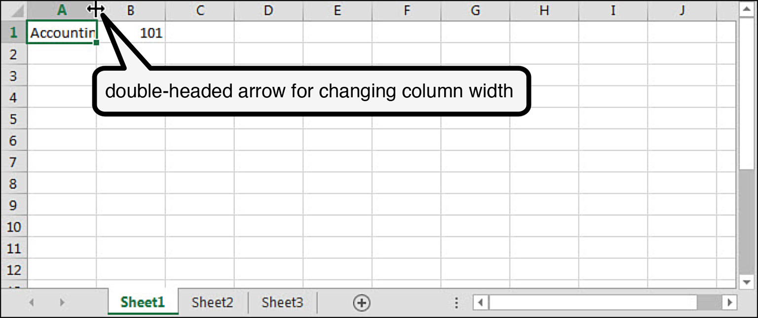
To widen a column to the width of the longest cell entry, double-click when your cursor changes to a double-headed arrow.

Spreadsheets exhibit a different behavior when a column isn’t wide enough to display an entire number. In some cases, you’ll see a series of pound signs (#) in the affected cells. They vanish when you make the column wide enough.

Let’s put together a simple exercise in Excel 2013 that will enable you to get a feel for spreadsheets. Our example spreadsheet helps you develop an amortization table to determine the cost of borrowing money for your business. This allows you to determine monthly payment and total interest cost to finance a car, another piece of equipment, or any other business need.

BOTTOM LINE

In reality, you’ll probably never actually need to build an amortization spreadsheet like this because ready-made templates abound. But following through the steps gives you some general exposure to what’s possible with spreadsheets. Many other templates can help you create other types of financial and business spreadsheets.

First, start a new, blank spreadsheet. This often appears automatically when you launch your spreadsheet program or app, but you might have to choose New or Blank Workbook.

This amortization schedule is first going to require that you store some assumptions needed to calculate the monthly payment. As noted, spreadsheets are broken down into cells, and just like houses, every cell has an address. The first cell in the upper-left corner is cell A1. In this cell, type Interest. When you press the Enter key, the next cell below, A2, is activated. The active cell in a spreadsheet always has a bold border around it.

Next type Term in cell A2, Loan in cell A3, and Payment in cell A4.

You now need to input some numbers into your spreadsheet, specifically an interest rate in cell B1. The interest rate for this example is 5.25 percent. You can enter this number in two ways: .0525 or 5.25%. If you choose the former, 0.0525 will appear in the spreadsheet. Spreadsheets automatically add leading zeros to decimal-based numbers such as an interest rate, but there’s no other formatting such as dollar signs or commas. This can make numbers hard to read, but you can add various types of formatting to remedy this.

In this case, if you click cell B1 and then click the Percent Style button (with the percent sign %) on the Home tab, the number appears as 5%. You’ll then need to click the Increase Decimal button twice to display the full interest rate, as shown in the following screenshot.

Excel offers one-click access to the Percent Style, but you might have to expand the number of decimals.

BOTTOM LINE

In many spreadsheet programs, you can save time and make numbers easier to read by typing the formatting when you enter the number. For instance, instead of typing .0525, enter 5.25% in a cell. For dollar amounts, type $30,000. If you typed 30000, it can be tough to distinguish at a glance if you entered three hundred thousand, thirty thousand, or three thousand. When you click the Accounting Number Format ($) button on the Home tab, Excel adds the dollar signs but also adds two decimal places you may have to remove using the Decrease Decimal button.

To continue with our example, enter 48 in cell B2 and $30,000 in cell B3. For the moment, leave cell B4 blank. Instead, move down to row 6 and type the following words in cells A6 through E6:

Period

Date

Interest

Principal

Balance

Enter the number 1 in cell A7.

At this point, cell A8 should be selected. That’s where we’ll enter our first formula.

DEFINITION

In a spreadsheet, a formula performs a calculation. You can always distinguish a formula for other types of inputs by the equal sign (=) that sits at the start of the formula.

Entering Formulas and Filling Entries

In cell A8, type =A7+1. This formula tells Excel to add 1 to whatever value is in cell A7. Because A7 contains the value 1, when you press Enter, the number 2 should appear in cell A8.

When typing cell addresses, you don’t need to worry about capitalization because =a7+1 and =A7+1 mean the same thing to Excel. In fact, you’ll notice that the spreadsheet software automatically capitalizes column letters when you press Enter.

At this point, you need to create a series of numbers from 1 to 48. However, you don’t need to type the formula that appears in cell A8 46 more times. Instead, you can use a feature that lets you replicate the formula by simply dragging with your mouse. To do so, click on cell A8 and notice the little square in the lower-right corner. This is the Fill Handle. If you position your mouse over the handle and drag down while holding down your left mouse button, Excel copies the formula for you. Drag down and stop at row 54. When you release your mouse button, you should see a series of numbers from 1 to 48.

Excel’s Fill Handle serves multiple purposes, including allowing you to copy data and formulas down a column or across a row.

Next, you’ll create a series of dates. In this case, you won’t use a formula, but instead create a series of numbers. In cell B7, enter 1/1/2019 to indicate the loan will commence as of January 1, 2019.

RED FLAG

Be careful not to include an equal sign when entering dates like you do when entering formulas. If you enter =1/1/2019, Excel will interpret that as a formula that should divide 1 by 1 by 2019, for a result of 0.000495. Or you might find that 1/1/2019 appears as the number 43466. Many spreadsheets use a convention where, behind the scenes, dates are represented by the number of days since January 1, 1900. January 1, 2019 falls 43,466 days after the turn of the previous century.

Next, enter 2/1/2019 in cell B8. You’ll now use a shortcut to complete the series of dates. Drag over cells B7 and B8 with your mouse to select both cells. Double-click on the Fill Handle, and Excel will populate the entire column of dates down to row 54. Alternatively, you could drag the fill handle as you did previously, but double-clicking is faster and easier.

To use this trick, you do have to select two cells to seed the series. If you only select one cell and double-click, you’d copy 2/1/19 all the way down the column.

Widen column B slightly if you find that certain cells are filled with # symbols.

Inserting a Function

Let’s move on to working with spreadsheet functions. As you’ve seen, spreadsheets allow you to carry out calculations in cells. Some calculations are simple, as in division, multiplication, addition, and subtraction. Other calculations can’t be carried out with simple arithmetic, such as a loan payment. Or if they could be carried out by hand, it would involve many cells and inputs. You can use functions in a spreadsheet formula to perform complicated calculations in a single cell.

Most spreadsheet programs have hundreds of functions available, so it can be daunting to determine if there’s an easier way to perform a calculation. We’ll walk you through each step.

First, click the cell where you want the formula—B4 in this case. Next, click the Formulas tab at the top of Excel and then click the Insert Function (fx) button in the Function Library group to display the Insert Function dialog box, shown next. Type what you’d like to do in the Search for a function: field, such as loan payment. Click Go, and the Select a function: list will show potential spreadsheet functions. In this case, the PMT function appears first on the list, and that’s what you need to calculate your loan payment. Click OK to use this function.

The Insert Function dialog box helps you determine if a function is available for a particular type of calculation.

At this point, a Function Arguments dialog box appears, which breaks down the input requirements for the function. Along the left side, you’ll see Rate, Nper, and PV in bold, while Fv and Type are not bolded. Required inputs are bolded; optional ones are not.

Excel can calculate the monthly payment for your loan if you instruct it where the inputs are:

• Rate: This is the interest rate in cell B1, which must be divided by 12 to arrive at the monthly rate, so enter B1/12.
• Nper: This is the length of the loan, otherwise knows as the term, which appears in cell B2, so enter B2.
• Pv: This is how much you want to borrow, or the loan amount in cell B3, so enter B3.

RED FLAG

Banks calculate loan interest on a monthly basis when applying the interest to your payments, but state the interest on an annual basis, so always be sure to convert annual interest rates to monthly amounts in spreadsheet formulas. In this case, enter =B1/12 in the Rate field to convert the annual interest rate of 5.25% (which appears in cell B1) to a monthly amount. If you forget to divide by 12, Excel will compute the loan as incurring 5.25% interest per month, or 63% per year, which means your loan payment will appear to be outrageous.

The Function Arguments dialog box identifies required versus optional inputs when crafting formulas that involve spreadsheet functions.

Once you’ve filled in the function arguments, the formula result returns -694.2813825. This is because Microsoft Excel calculates values to as many as 15 decimal places (only 7 decimal places were required for this calculation). However, in your spreadsheet, you can format the number to only show 2 decimal places. Click OK to place the formula in cell B4.

Now, ($694.28) should appear in cell B4. The parentheses indicate this is a negative number. Excel’s PMT function returns a negative value because it considers the loan payment to be an outflow. Leaving this number as a negative value complicates some of the other formulas you need to add to the spreadsheet, so let’s change it to a positive value. To do so, double-click on cell B4, which enables you to edit the formula. Add a minus sign (-) just after the equal sign so the formula reads =-B1/12, and press Enter.

Finishing the Amortization Table Formulas

You’re now ready to build the rest of the amortization table. Click on cell C7, and enter this formula:

=B3*B1/12

In plain English, this means multiply $30,000 from cell B3 by 5.25% (the interest rate in cell B1) and divide the result by 12.

Your formula should return $131.25, which means $131.25 of your first month’s payment of $694.28 goes to the bank as interest.

Next, enter this formula in cell D7:

=B$4-C7

Your formula should return $563.03. You’ll notice this formula includes a dollar sign, which has special significance to Excel. If you refer to the formulas in cells A8 to A54, you’ll see that as you copied the formula down, Excel changed each row number automatically. That’s the natural process, and that’s what you want for these formulas. In this case, you always need to refer to cell B4, so adding dollar signs instructs Excel not to change row 4 to a 5 if you were to copy the formula down a row. In spreadsheet parlance, this is known as an absolute reference.

DEFINITION

Most spreadsheet formulas involve relative references, which mean column letters and row numbers increment automatically as you copy a formula down a column or across a row. An absolute reference instructs Excel not to change the column letter and/or row number when you copy the formula. Place dollar signs as needed in formulas to prevent column letter and row number changes.

This brings you to cell E7, where you’ll calculate the ending balance as of each month:

=B3-D7

The formula should return $29,436.97, which is the amount you’ll still owe on the loan after the first month’s payment. You’re now ready to add the second row of formulas, after which you’ll be able to copy the formulas down the rest of the column.

Enter this formula in cell C8:

=E7*B$1/12

The formula should return $128.79. This amount is slightly less than the interest for the first month because you’ve paid down the loan slightly. For the first month, you based this calculation on the initial loan balance of $30,000, but going forward, interest will be based on the ending balance for the previous month. A dollar sign in the formula instructs Excel to always refer to row 1, where the interest rate is, as you’ll be copying this formula down the rest of the column.

In that regard, you don’t need to actually write a formula in cell D8. You can use the Fill Handle to drag the formula in cell D7 into cell D8.

For cell E8, you’ll enter this formula:

=E7-D8

There are no dollar signs in this formula because you want to refer to the ending balance for the previous month, as well as the amount you paid down in the current month. If you want to check your work, cell D8 should return $565.49 and cell E8 should return $28,871.47.

At this point, you’re ready to populate the rest of the amortization table, but you don’t need to write any more formulas to do so. Simply select cells C8 through E8 with your mouse, and double-click the Fill Handle in cell E8. Excel will copy the formulas down through row 54, stopping just before it encounters a blank cell in column B. Cell E54 should return 0, because at that point, the loan will be fully repaid.

If this isn’t the case for you, check each of your formulas by double-clicking on the respective cells. Most likely, you’ll find you omitted or misplaced a dollar sign to create an absolute reference back to one of the assumption cells.

Freezing Rows On-Screen

As we noted earlier, spreadsheets can house astronomical amounts of data, but it’s easy to get lost even in the small spreadsheet you just created. When you scroll down to row 54, you could lose sight of the column headings you added in row 6. However, you don’t have to sift aimlessly through columns of numbers; you can freeze certain rows on-screen.

To freeze the rows containing your titles, scroll your spreadsheet up until you get to row 1. You can use the scroll bar on the right-hand side of the screen, or press Ctrl+Home on your keyboard. Next, click on cell A7 in preparation for freezing rows 1 through 6 on-screen. Click the View tab at the top of Excel, choose Freeze Panes in the Window group, and choose Freeze Panes again. Now, when you scroll down either with the scroll bar or by pressing the down arrow or Page Down keys, rows 1 through 6 always remain on your screen. You can use the same steps to unfreeze the rows. You’ll see the Freeze Panes command has changed to Unfreeze Panes.

You can use the Freeze Panes command to prevent rows with titles from scrolling off screen.

You’ll add one more type of formula to your amortization schedule and print the data. Select cells C55 and D55 with your mouse. Click the Home tab, and click the AutoSum button (Σ) in the Editing group. This adds the SUM spreadsheet function to both cells, and that shows the total interest and principal you’ll pay over the course of the loan. You’ll likely need to widen columns C and D slightly to show the totals of $3,325.51 and $30,000.00 respectively.

The AutoSum feature allows you to sum rows or columns with the click of your mouse.

Printing

Earlier, you froze rows 1 through 6 on the screen, but you’ll need to take a different approach to freeze these rows on your printout. To do so, click on the Page Layout tab in Excel’s ribbon, and click the Print Titles button in the Page Setup group. Enter 1:6 in the Rows to Repeat at Top text box, and click the Print or Print Preview button to print your amortization schedule or click OK to close the dialog box without printing.

You can easily set certain rows to appear at the top of each page of your printouts.

In this chapter, we were only able to scratch the surface of what’s possible with spreadsheets, but now you should have a good idea of how to get started using Excel. In the next chapter, we look at some other ways you can use spreadsheets. If this is all new terrain for you, we recommend you refer to Idiot’s Guides: Microsoft Excel 2013 by Michael Miller.

The Least You Need to Know

• Microsoft Excel is the most popular spreadsheet program, but other options are available, some of them free.
• Spreadsheets are electronic versions of accountant’s ledger paper that are capable of carrying out calculations.
• An amortization schedule is just one of many ways you can use spreadsheets to calculate numbers related to your business.