![]()
Introducing Microsoft Azure Machine Learning
Azure Machine Learning, where data science, predictive analytics, cloud computing, and your data meet!
Azure Machine Learning empowers data scientists and developers to transform data into insights using predictive analytics. By making it easier for developers to use the predictive models in end-to-end solutions, Azure Machine Learning enables actionable insights to be gleaned and operationalized easily.
Using Machine Learning Studio, data scientists and developers can quickly build, test, and develop the predictive models using state-of-the art machine learning algorithms.
Hello, Machine Learning Studio!
Azure Machine Learning Studio provides an interactive visual workspace that enables you to easily build, test, and deploy predictive analytic models.
In Machine Learning Studio, you construct a predictive model by dragging and dropping datasets and analysis modules onto the design surface. You can iteratively build predictive analytic models using experiments in Azure Machine Learning Studio. Each experiment is a complete workflow with all the components required to build, test, and evaluate a predictive model. In an experiment, machine learning modules are connected together with lines that show the flow of data and parameters through the workflow. Once you design an experiment, you can use Machine Learning Studio to execute it.
Machine Learning Studio allows you to iterate rapidly by building and testing several models in minutes. When building an experiment, it is common to iterate on the design of the predictive model, edit the parameters or modules, and run the experiment several times. Often, you will save multiple copies of the experiment (using different parameters). When you first open Machine Learning Studio, you will notice it is organized as follows:
- Experiments: Experiments that have been created, run, and saved as drafts. These include a set of sample experiments that ship with the service to help jumpstart your projects.
- Web Services: A list of experiments that you have published as web services. This list will be empty until you publish your first experiment.
- Settings: A collection of settings that you can use to configure your account and resources. You can use this option to invite other users to share your workspace in Azure Machine Learning.
To develop a predictive model, you will need to be able to work with data from different data sources. In addition, the data needs to be transformed and analyzed before it can be used as input for training the predictive model. Various data manipulation and statistical functions are used for preprocessing the data and identifying the parts of the data that are useful. As you develop a model, you go through an iterative process where you use various techniques to understand the data, the key features in the data, and the parameters that are used to tune the machine learning algorithms. You continuously iterate on this until you get to point where you have a trained and effective model that can be used.
Components of an Experiment
An experiment is made of the key components necessary to build, test, and evaluate a predictive model. In Azure Machine Learning, an experiment contains two main components: datasets and modules.
A dataset contains data that has been uploaded to Machine Learning Studio. The dataset is used when creating a predictive model. Machine Learning Studio also provides several sample datasets to help you jumpstart the creation of your first few experiments. As you explore Machine Learning Studio, you can upload additional datasets.
A module is an algorithm that you will use when building your predictive model. Machine Learning Studio provides a large set of modules to support the end-to-end data science workflow, from reading data from different data sources; preprocessing the data; to building, training, scoring, and validating a predictive model. These modules include the following:
- Convert to ARFF: Converts a .NET serialized dataset to ARFF format.
- Convert to CSV: Converts a .NET serialized dataset to CSV format.
- Reader: This module is used to read data from several sources including the Web, Azure SQL Database, Azure Blob storage, or Hive tables.
- Writer: This module is used to write data to Azure SQL Database, Azure Blob storage, or Hadoop Distributed File system (HDFS).
- Moving Average Filter: This creates a moving average of a given dataset.
- Join: This module joins two datasets based on keys specified by the user. It does inner joins, left outer joins, full outer joins, and left semi-joins of the two datasets.
- Split: This module splits a dataset into two parts. It is typically used to split a dataset into separate training and test datasets.
- Filter-Based Feature Selection: This module is used to find the most important variables for modeling. It uses seven different techniques (e.g. Spearman Correlation, Pearson Correlation, Mutual Information, Chi Squared, etc.) to rank the most important variables from raw data.
- Elementary Statistics: Calculates elementary statistics such as the mean, standard deviation, etc., of a given dataset.
- Linear Regression: Can be used to create a predictive model with a linear regression algorithm.
- Train Model: This module trains a selected classification or regression algorithm with a given training dataset.
- Sweep Parameters: For a given learning algorithm, along with training and validation datasets, this module finds parameters that result in the best trained model.
- Evaluate Model: This module is used to evaluate the performance of a trained classification or regression model.
- Cross Validate Model: This module is used to perform cross-validation to avoid over fitting. By default this module uses 10-fold cross-validation.
- Score Model: Scores a trained classification or regression model.
All available modules are organized under the menus shown in Figure 2-1. Each module provides a set of parameters that you can use to fine-tune the behavior of the algorithm used by the module. When a module is selected, you will see the parameters for the module displayed on the right pane of the canvas.
Five Easy Steps to Creating an Experiment
In this section, you will learn how to use Azure Machine Learning Studio to develop a simple predictive analytics model. To design an experiment, you assemble a set of components that are used to create, train, test, and evaluate the model. In addition, you might leverage additional modules to preprocess the data, perform feature selection and/or reduction, split the data into training and test sets, and evaluate or cross-validate the model. The following five basic steps can be used as a guide for creating an experiment.
Create a Model
- Step 1: Get data
- Step 2: Preprocess data
- Step 3: Define features
Train the Model
- Step 4: Choose and apply a learning algorithm
Test the Model
- Step 5: Predict over new data
Step 1: Get Data
Azure Machine Learning Studio provides a number of sample datasets. In addition, you can also import data from many different sources. In this example, you will use the included sample dataset called Automobile price data (Raw), which represents automobile price data.
- To start a new experiment, click +NEW at the bottom of the Machine Learning Studio window and select EXPERIMENT.
- Rename the experiment to “Chapter 02 – Hello ML”.
- To the left of the Machine Learning Studio, you will see a list of experiment items (see Figure 2-1). Click Saved Datasets, and type “automobile” in the search box. Find Automobile price data (Raw).

Figure 2-1. Palette search
- Drag the dataset into the experiment. You can also double-click the dataset to include it in the experiment (see Figure 2-2).
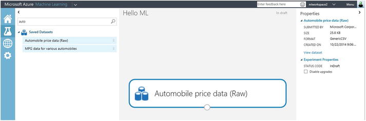
Figure 2-2. Using a dataset
By clicking the output port of the dataset, you can select Visualize, which will allow you to explore the data and understand the key statistics of each of the columns (see Figure 2-3).

Figure 2-3. Dataset visualization
Close the visualization window by clicking the x in the upper-right corner.
Step 2: Preprocess Data
Before you start designing the experiment, it is important to preprocess the dataset. In most cases, the raw data needs to be preprocessed before it can be used as input to train a predictive analytic model.
From the earlier exploration, you may have noticed that there are missing values in the data. As a precursor to analyzing the data, these missing values need to be cleaned. For this experiment, you will substitute the missing values with a designated value. In addition, the normalized-losses column will be removed as this column contains too many missing values.
![]() Tip Cleaning the missing values from input data is a prerequisite for using most of the modules.
Tip Cleaning the missing values from input data is a prerequisite for using most of the modules.
- To remove the normalized-losses column, drag the Project Columns module, and connect it to the output port of the Automobile price data (Raw) dataset. This module allows you to select which columns of data you want to include or exclude in the model.
- Select the Project Columns module and click Launch column selector in the properties pane (i.e. the right pane).
- Make sure All columns is selected in the filter dropdown called Begin With. This directs Project Columns to pass all columns through (except for the ones you are about to exclude).
- In the next row, select Exclude and column names, and then click inside the text box. A list of columns is displayed; select “normalized-losses” and it will be added to the text box. This is shown in Figure 2-4.
- Click the check mark OK button to close the column selector.
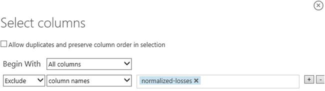
Figure 2-4. Select columns
All columns will pass through, except for the column normalized-losses. You can see this in the properties pane for Project Columns. This is illustrated in Figure 2-5.
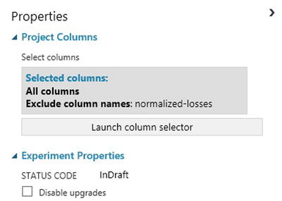
Figure 2-5. Project Columns properties
 Tip As you design the experiment, you can add a comment to the module by double-clicking the module and entering text. This enables others to understand the purpose of each module in the experiment and can help you document your experiment design.
 - Drag the Missing Values Scrubber module to the experiment canvas and connect it to the Project Columns module. You will use the default properties, which replaces the missing value with a 0. See Figure 2-6 for details.

Figure 2-6. Missing Values Scrubber properties
- Now click RUN.
- When the experiment completes successfully, each of the modules will have a green check mark indicating its successful completion (see Figure 2-7).

Figure 2-7. First experiment run
At this point, you have preprocessed the dataset by cleaning and transforming the data. To view the cleaned dataset, double-click the output port of the Missing Values Scrubber module and select Visualize. Notice that the normalized-losses column is no longer included, and there are no missing values.
Step 3: Define Features
In machine learning, features are individual measurable properties created from the raw data to help the algorithms to learn the task at hand. Understanding the role played by each feature is super important. For example, some features are better at predicting the target than others. In addition, some features can have a strong correlation with other features (e.g. city-mpg vs. highway-mpg). Adding highly correlated features as inputs might not be useful, since they contain similar information.
For this exercise, you will build a predictive model that uses a subset of the features of the Automobile price data (Raw) dataset to predict the price for new automobiles. Each row represents an automobile. Each column is a feature of that automobile. It is important to identify a good set of features that can be used to create the predictive model. Often, this requires experimentation and knowledge about the problem domain. For illustration purpose, you will use the Project Columns module to select the following features: make, body-style, wheel-base, engine-size, horsepower, peak-rpm, highway-mpg, and price.
- Drag the Project Columns module to the experiment canvas. Connect it to the Missing Values Scrubber module.
- Click Launch column selector in the properties pane.
- In the column selector, select No columns for Begin With, then select Include and column names in the filter row. Enter the following column names: make, body-style, wheel-base, engine-size, horsepower, peak-rpm, highway-mpg, and price. This directs the module to pass through only these columns.
- Click OK.
![]() Tip As you build the experiment, you will run it. By running the experiment, you enable the column definitions of the data to be used in the Missing Values Scrubber module.
Tip As you build the experiment, you will run it. By running the experiment, you enable the column definitions of the data to be used in the Missing Values Scrubber module.
When you connect Project Columns to Missing Values Scrubber, the Project Columns module becomes aware of the column definitions in your data. When you click the column names box, a list of columns is displayed and you can then select the columns, one at a time, that you wish to add to the list.

Figure 2-8. Select columns
Figure 2-8 shows the list of selected columns in the Project Columns module. When you train the predictive model, you need to provide the target variable. This is the feature that will be predicted by the model. For this exercise, you are predicting the price of an automobile, based on several key features of an automobile (e.g. horsepower, make, etc.)
Step 4: Choose and Apply Machine Learning Algorithms
When constructing a predictive model, you first need to train the model, and then validate that the model is effective. In this experiment, you will build a regression model.
![]() Tip Classification and regression are two common types of predictive models. In classification, the goal is to predict if a given data row belongs to one of several classes (e.g. will a customer churn or not? Is this credit transaction fraudulent?). With regression, the goal is to predict a continuous outcome (e.g. the price of an automobile or tomorrow’s temperature).
Tip Classification and regression are two common types of predictive models. In classification, the goal is to predict if a given data row belongs to one of several classes (e.g. will a customer churn or not? Is this credit transaction fraudulent?). With regression, the goal is to predict a continuous outcome (e.g. the price of an automobile or tomorrow’s temperature).
In this experiment, you will train a regression model and use it to predict the price of an automobile. Specifically, you will train a simple linear regression model. After the model has been trained, you will use some of the modules available in Machine Learning Studio to validate the model.
- Split the data into training and testing sets: Select and drag the Split module to the experiment canvas and connect it to the output of the last Project Columns module. Set Fraction of rows in the first output dataset to 0.8. This way, you will use 80% of the data to train the model and hold back 20% for testing.
Tip By changing the Random seed parameter, you can produce different random samples for training and testing. This parameter controls the seeding of the pseudo-random number generator in the Split module.
- Run the experiment. This allows the Project Columns and Split modules to pass along column definitions to the modules you will be adding next.
- To select the learning algorithm, expand the Machine Learning category in the module palette to the left of the canvas and then expand Initialize Model. This displays several categories of modules that can be used to initialize a learning algorithm.
- For this example experiment, select the Linear Regression module under the Regression category and drag it to the experiment canvas.
- Find and drag the Train Model module to the experiment. Click Launch column selector and select the price column. This is the feature that your model is going to predict. Figure 2-9 shows this target selection.

Figure 2-9. Select the price column
- Connect the output of the Linear Regression module to the left input port of the Train Model module.
- Also, connect the training data output (i.e. the left port) of the Split module to the right input port of the Train Model module.
- Run the experiment.
The result is a trained regression model that can be used to score new samples to make predictions. Figure 2-10 shows the experiment up to Step 7.

Figure 2-10. Applying the learning algorithm
Step 5: Predict Over New Data
Now that you’ve trained the model, you can use it to score the other 20% of your data and see how well your model predicts on unseen data.
- Find and drag the Score Model module to the experiment canvas and connect the left input port to the output of the Train Model module, and the right input port to the test data output (right port) of the Split module. See Figure 2-11 for details.

Figure 2-11. Score Model module
- Run the experiment and view the output from the Score Model module (by double-clicking the output port and selecting Visualize). The output will show the predicted values for price along with the known values from the test data.
- Finally, to test the quality of the results, select and drag the Evaluate Model module to the experiment canvas, and connect the left input port to the output of the Score Model module (there are two input ports because the Evaluate Model module can be used to compare two different models).
- Run the experiment and view the output from the Evaluate Model module (double-click the output port and select Visualize). The following statistics are shown for your model:
- Mean Absolute Error (MAE): The average of absolute errors (an error is the difference between the predicted value and the actual value).
- Root Mean Squared Error (RMSE): The square root of the average of squared errors.
- Relative Absolute Error: The average of absolute errors relative to the absolute difference between actual values and the average of all actual values.
- Relative Squared Error: The average of squared errors relative to the squared difference between the actual values and the average of all actual values.
- Coefficient of Determination: Also known as the R squared value, this is a statistical metric indicating how well a model fits the data.
For each of the error statistics, smaller is better; a smaller value indicates that the predictions more closely match the actual values. For Coefficient of Determination, the closer its value is to one (1.0), the better the predictions (see Figure 2-12). If it is 1.0, this means the model explains 100% of the variability in the data, which is pretty unrealistic!
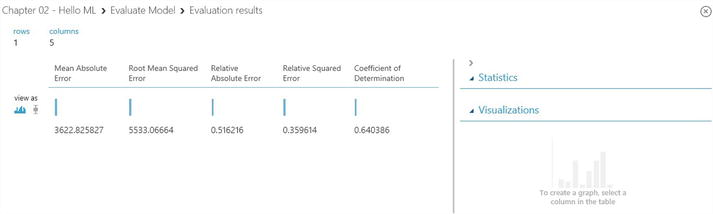
Figure 2-12. Evaluation results
The final experiment should look like the screenshot in Figure 2-13.
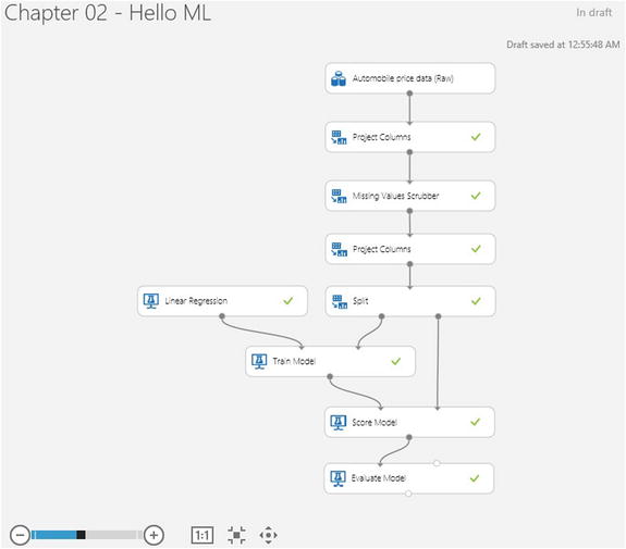
Figure 2-13. Regression Model experiment
Congratulations! You have created your first machine learning experiment in Machine Learning Studio. In Chapters 5-8, you will see how to apply these five steps to create predictive analytics solutions that address business challenges from different domains such as buyer propensity, churn analysis, customer segmentation, and predictive maintenance. In addition, Chapter 3 shows how to use R scripts as part of your experiments in Azure Machine Learning.
Deploying Your Model in Production
Today it takes too long to deploy machine learning models in production. The process is typically inefficient and often involves rewriting the model to run on the target production platform, which is costly and requires considerable time and effort. Azure Machine Learning simplifies the deployment of machine learning models through an integrated process in the cloud. You can deploy your new predictive model in a matter of minutes instead of days or weeks. Once deployed, your model runs as a web service that can be called from different platforms including servers, laptops, tablets, or even smartphones. To deploy your model in production follow these two steps.
- Deploy your model to staging in Azure Machine Learning Studio.
- In Azure Management portal, move your model from the staging environment into production.
Deploying Your Model into Staging
To deploy your model into staging, follow these steps in Azure Machine Learning Studio.
- Save your trained mode using the Save As button at the bottom of Azure Machine Learning Studio. Rename it to a new name of your choice.
- Run the experiment.
- Right-click the output of the training module (e.g. Train Model) and select the option Save As Trained Model.
- Delete any modules that were used for training (e.g. Split, Train Model, Evaluate Model).
- Connect the newly saved model directly to the Score Model module.
- Rerun your experiment.
- Before the deletion in Step 1c your experiment should appear as shown Figure 2-14.

Figure 2-14. Predictive model before the training modules were deleted
After deleting the training modules (i.e. Split, Linear Regression, Train Model, and Evaluate Model) and then replacing those with the saved training model, the experiment should now appear as shown in Figure 2-15.
Tip You may be wondering why you left the Automobile price data (Raw) dataset connected to the model. The service is going to use the user’s data, not the original dataset, so why leave them connected?It’s true that the service doesn’t need the original automobile price data. But it does need the schema for that data, which includes information such as how many columns there are and which columns are numeric. This schema information is necessary in order to interpret the user’s data. You leave these components connected so that the scoring module will have the dataset schema when the service is running. The data isn’t used, just the schema.

Figure 2-15. The experiment that uses the saved training model
- Next, set your publishing input and output. To do this, follow these steps.
- Right-click the right input of the module named Score Model. Select the option Set As Publish Input.
- Right-click the output of the Score Model module and select Set As Publish Output.
After these two steps you will see two circles highlighting the chosen publish input and output on the Score Model module. This is shown in Figure 2-15.
- Once you assign the publish input and output, run the experiment and then publish it into staging by clicking Publish Web Service at the bottom of the screen.
![]() Tip You can update the web service after you’ve published it. For example, if you want to change your model, just edit the training experiment you saved earlier, tweak the model parameters, and save the trained model (overwriting the one you saved before). When you open the scoring experiment again, you’ll see a notice telling you that something has changed (that will be your trained model) and you can update the experiment. When you publish the experiment again, it will replace the web service, now using your updated model.
Tip You can update the web service after you’ve published it. For example, if you want to change your model, just edit the training experiment you saved earlier, tweak the model parameters, and save the trained model (overwriting the one you saved before). When you open the scoring experiment again, you’ll see a notice telling you that something has changed (that will be your trained model) and you can update the experiment. When you publish the experiment again, it will replace the web service, now using your updated model.
You can configure the service by clicking the Configuration tab. Here you can modify the service name (it’s given the experiment name by default) and give it a description. You can also give more friendly labels for the input and output columns.
Testing the Web Service
On the Dashboard page, click the Test link under Staging Services. A dialog will pop up that asks you for the input data for the service. These are the same columns that appeared in the original Automobile price data (Raw) dataset. Enter a set of data and then click OK.
The results generated by the web service are displayed at the bottom of the dashboard. The way you have the service configured, the results you see are generated by the scoring module.
Moving Your Model from Staging into Production
At this point your model is now in staging, but is not yet running in production. To publish it in production you need to move it from the staging to the production environment through the following steps.
- Configure your new web service in Azure Machine Learning Studio and make it ready for production as follows.
- In Azure Machine Learning Studio, click the menu called Web Services on the right pane. It will show a list of all your web services.
- Click the name of the new service you just created. You can test it by clicking the Test URL.
- Now click the configuration tab, and then select yes for the option Ready For Production? Then click the Save button at the bottom of the screen. Now your model is ready to be published in production.
- Now switch to the Azure Management Portal and publish your web service into production as follows.
- Select Machine Learning on the left pane in Azure Management Portal.
- Choose the workspace with the experiment you want to deploy in production.
- Click on the name of your workspace, and then click the tab named Web Services.
- Choose the +Add button at the bottom of the Azure Management Portal window.
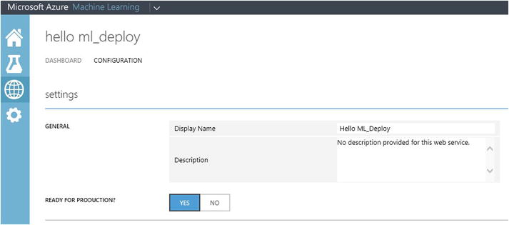
Figure 2-16. A dialog box that promotes the machine learning model from the staging server to a live production web service
Congratulations! You have just published your very first machine learning model into production. If you click your model from the Web Services tab, you will see details such as the number of predictions made by your model over a seven-day window. The service also shows the APIs you can use to call your model as a web service either in a request/response or batch execution mode. As if this is not enough, you also get sample code you can use to invoke your new web service in C#, Python, or R. You can use this sample code to call your model as a web service from a web form in a browser or from any other application of your choice.
Accessing the Azure Machine Learning Web Service
To be useful as a web service, users need to be able to send data to the service and receive results. The web service is an Azure web service that can receive and return data in one of two ways:
- Request/Response: The user can send a single set of Automobile price data to the service using an HTTP protocol, and the service responds with a single result predicting the price.
- Batch Execution: The user can send to the service the URL of an Azure BLOB that contains one or more rows of Automobile price data. The service stores the results in another BLOB and returns the URL of that container.
On the Dashboard tab for the web service, there are links to information that will help a developer write code to access this service. Click the API help page link on the REQUEST/RESPONSE row and a page opens that contains sample code to use the service’s request/response protocol. Similarly, the link on the BATCH EXECUTION row provides example code for making a batch request to the service.
The API help page includes samples for R, C#, and Python programming languages. For example, Listing 2-1 shows the R code that you could use to access the web service you published (the actual service URL would be displayed in your sample code).
Listing 2-1. R Code Used to Access the Service Programmatically
library("RCurl")
library("RJSONIO")

# Accept SSL certificates issued by public Certificate Authorities
options(RCurlOptions = list(sslVersion=3L, cainfo = system.file("CurlSSL", "cacert.pem", package = "RCurl")))

h = basicTextGatherer()
req = list(Id="score00001",
 Instance=list(FeatureVector=list(
    "symboling"= "0",
    "make"= "0",
    "body-style"= "0",
    "wheel-base"= "0",
    "engine-size"= "0",
    "horsepower"= "0",
    "peak-rpm"= "0",
    "highway-mpg"= "0",
    "price"= "0"
 ),GlobalParameters=fromJSON('{}')))

body = toJSON(req)
api_key = "abc123" # Replace this with the API key for the web service
authz_hdr = paste('Bearer', api_key, sep=' ')

h$reset()
curlPerform(url = "https://ussouthcentral.services.azureml.net/workspaces/fcaf778fe92f4fefb2f104acf9980a6c/services/ca2aea46a205473aabca2670c5607518/score",
            httpheader=c('Content-Type' = "application/json", 'Authorization' = authz_hdr),
            postfields=body,
            writefunction = h$update,
            verbose = TRUE
            )

result = h$value()
print(result)
Summary
In this chapter, you learned how to use Azure Machine Learning Studio to create your first experiment. You saw how to perform data preprocessing, and how to train, test, and evaluate your model in Azure Machine Learning Studio. In addition, you also saw how to deploy your new model in production. Once deployed, your machine learning model runs as a web service on Azure that can be called from a web form or any other application from a server, laptop, tablet, or smartphone. In the remainder of this book, you will learn how to use Azure Machine Learning to create experiments that solve various business problems such as customer propensity, customer churn, and predictive maintenance. In addition, you will also learn how to extend Azure Machine Learning with R scripting. Also, Chapter 4 introduces the most commonly used statistics and machine learning algorithms in Azure Machine Learning.