![]()
The question is, “Where do I start?” In the beginning, Codd created the paper “A Relational Model of Data for Large Shared Data Banks.” Now the relational database was formless and empty, darkness was over the surface of the media, and the spirit of Codd was hovering over the requirements. Codd said, “Let there be Alpha,” but as usual, the development team said, “Let there be something else,” so SEQUEL (SQL) was created. Codd saw that SQL wasn’t what he had in mind, but it was too late, for the Ellison separated the darkness from the SQL and called it Oracle. OK, that’s enough of that silliness. But that’s the short of it.
Did you know that about 25% of the average stored procedures written in the Procedural Language for SQL (PL/SQL) is, in fact, just SQL? Well, I’m a metrics junkie. I’ve kept statistics on every program I’ve ever written, and that’s the statistic. After writing more than 30,000 stored procedures, 26% of my PL/SQL is nothing but SQL. So it’s really important for you to know SQL!
OK, maybe you don’t know SQL that well after all. If not, continue reading this light-speed refresher on relational SQL. Otherwise, move on to the exercises in the last section of the chapter (“Your Working Example”).
This chapter covers Data Definition Language (DDL) and Data Manipulation Language (DML), from table creation to queries. Please keep in mind that this chapter is not a tutorial on SQL. It’s simply a review. SQL is a large topic that can be covered fully only with several books. What I’m trying to accomplish here is to help you determine how familiar you are with SQL, so you’ll be able to decide whether you need to spend some additional time learning SQL after or while you learn PL/SQL.
Tables
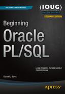
The core idea behind a relational database and SQL is so simple it’s elusive. Take a look at Tables 1-1 and 1-2.
Table 1-1. Relational Database Geniuses (Authors)
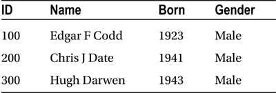
Table 1-2. Relational Genius’s Publications (Author Publications)
You can find which publications were written by each genius simply by using the common datum in both of these tables: the ID. If you look at Codd’s data in Table 1-1, you see he has ID 100. Next, if you look at ID 100’s (Codd’s) data in Table 1-2, you see he has written two titles:
- A Relational Model of Data for Large Shared Data Banks (1970)
- The Relational Model for Database Management (1990)
These two tables have a relationship, because they share an ID column with the same values. They don’t have many entries, so figuring out what was written by each author is pretty easy. But what would you do if there were, say, one million authors with about three publications each? Yes! It’s time for a computer and a database—a relational database.
A relational database allows you to store multiple tables, like Tables 1-1 and 1-2, in a database management system (DBMS). By doing so, you can manipulate the data in the tables using a query language on a computer, instead of a pencil on a sheet of paper. The current query language of choice is Structured Query Language (SQL). SQL is a set of nonprocedural commands, or language if you will, which you can use to manipulate the data in tables in a relational database management system (RDBMS).
A table in a relational database is a logical definition for how data is to be organized when it is stored. For example, in Table 1-3, I decided to order the columns of the database genius data just as it appeared horizontally in Table 1-1.
Table 1-3. A Table Definition for Table 1-1
Column Number | Column Name | Data Type |
|---|---|---|
1 | ID | Number |
2 | Name | Character |
3 | Birth Date | Date |
4 | Gender | Character |
Perhaps I could give the relational table defined in Table 1-3 the name geniuses? In practice, a name like that tends to be too specific. It’s better to find a more general name, like authors or persons. So how do you document your database design decisions?
An Entity-Relationship Diagram
Just as home builders have an architectural diagram or blueprint, which enables them to communicate clearly and objectively about what they are going to build, so do relational database builders. In our case, the architectural diagram is called an entity-relationship diagram (ERD).
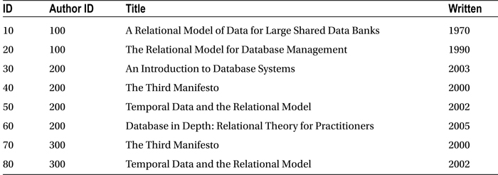
Figure 1-1 is an ERD for the tables shown in Tables 1-1 and 1-2, now named authors and author_publications. It shows that one author may have zero or more publications. Additionally, it shows that an author’s ID is his primary key (PK), or unique way to identify him, and an author’s primary key is also used to identify his publications.
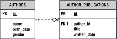
Figure 1-1. An entity-relationship diagram for the authors and author publications tables
ERDs, like blueprints, may have varying levels of detail, depending on your audience. For example, to simplify the ERD in Figure 1-1, I’ve left out the data types.
In an ERD, the tables are called entities. The lines that connect the tables—I mean entities—are called relations. So given an ERD, or even a narrative documentation as in Table 1-3, you can write a script to create a table.
Data Definition Language (DDL)
To create the authors table, as defined in Table 1-3, in Oracle, you’ll need to create a SQL script (for SQL*Plus) that in SQL jargon is called Data Definition Language. That is, it’s SQL for defining the relational database. Listing 1-1 shows the authors table’s DDL.
Listing 1-1. DDL for Creating the Author Table, authors.tab
1  CREATE TABLE authors (
2  id                             number(38),
3  name                           varchar2(100),
4  birth_date                     date,
5  gender                         varchar2(30) );
The syntax for the CREATE TABLE statement used in Listing 1-1 is as follows:
CREATE TABLE <table_name> (
<column_name_1>   <data_type_1>,
<column_name_2>   <data_type_2>,
<column_name_N>   <data_type_N> );
where <table_name> is the name of the table, <column_name> is the name of a column, and <data_type> is one of the Oracle data types.
The following are the Oracle data types you’ll use most often:
- VARCHAR2: Allows you to store up to 32,767 bytes (4,000 in versions prior to 12c) , data like ABCD..., in a column. You must define the maximum number of characters (or constrain the number of characters) by specifying the desired number in parentheses after the keyword VARCHAR2. For example, in Listing 1-1, line 3 specifies varchar2(100), which means a name can be up to 100 characters in length.
- NUMBER: Allows you to store a decimal number with 38 digits of precision. You do not need to constrain the size of a number, but you can. You can specify the maximum number of digits (1, 2, 3, 4 . . .) to the left of a decimal point, followed by a comma (,), and optionally the maximum number of decimal digits to the right of the decimal point, by specifying the desired constraint in parentheses after the keyword NUMBER. For example, if you want to make sure that the id column in Listing 1-1, line 2 is an integer, you could specify number(38).
- DATE: Allows you to store a date and time value. One great thing about Oracle DATE types is that they allow you to easily perform time calculations between dates; just subtract an earlier date from a later date. In addition, it’s also easy to convert between VARCHAR2 and DATE values. For example, if you want to store the date and time of birth for someone born on January 1, 1980 at 8 a.m., you could use the Oracle to_date() function to convert a VARCHAR2 value in a proper format into a DATE data type as follows: to_date('19800101080000', 'YYYYMMDDHH24MISS').
Of course, there are other Oracle data types, but you’ll end up using VARCHAR2, NUMBER, and DATE most of the time. The rest are specialized versions of these three, or they are designed for specialized uses.
It’s Your Turn to Create a Table
OK, it’s time to stop reading and start doing. This section gives you chance to put into practice some of what you’ve learned so far. I’ll be asking you to perform exercises like this as we go along in order for you to verify that you understood what you just read well enough to put it into practice.
![]() Tip First, if you don’t have access to Oracle, see this book’s appendix. Second, create a directory for the book’s source code listings. Next, download the source code listings from the Source Code/Download section of the Apress web site (www.apress.com), and work within the book’s source code listing directory structure for each chapter. Add your source code listings to the book’s directory structure as you work. Last, create a shortcut, an icon, or whatever you want to call it, to start SQL*Plus from your working source code listing directory. Then you won’t need to specify the entire path when trying to execute your scripts in SQL*Plus.
Tip First, if you don’t have access to Oracle, see this book’s appendix. Second, create a directory for the book’s source code listings. Next, download the source code listings from the Source Code/Download section of the Apress web site (www.apress.com), and work within the book’s source code listing directory structure for each chapter. Add your source code listings to the book’s directory structure as you work. Last, create a shortcut, an icon, or whatever you want to call it, to start SQL*Plus from your working source code listing directory. Then you won’t need to specify the entire path when trying to execute your scripts in SQL*Plus.
To create the author_publications table, follow these steps.
- Start your Oracle database if it’s not already running.
- Start SQL*Plus, logging in as username RPS with password RPS.
- Open your favorite text editor.
- Write a DDL script to create a table for author_publications, as in Table 1-2.
- Save the DDL script with the same filename as your table name, but with a .tab extension.
- Execute your script in SQL*Plus by typing an at sign (@) followed by the filename at the SQL> prompt.
If you didn’t have any errors in your script, the table will now exist in the database, just waiting for you to populate it with data. If it didn’t work, try to make some sense out of the error message(s) you got, correct your script, and then try again.
Listing 1-2 is my try.
Listing 1-2. DDL for Creating the Publication Table, author_publications.tab
1  CREATE TABLE author_publications (
2  id                             number(38),
3  title                          varchar2(100),
4  written_date                   date );
Now you know how to create a table, but what if you put a lot of data in those two tables? Then accessing them will be very slow, because none of the columns in the tables are indexed.
Indexes
Imagine, if you will, that a new phone book shows up on your doorstep. You put it in the drawer and throw out the old one. You pull the phone book out on Saturday evening so you can order some pizza, but when you open it, you get confused. Why? Well, when they printed the last set of phone books, including yours, they forgot to sort it by last name, first name, and street address. Instead, it’s not sorted at all! The numbers show up the way they were put into the directory over the years—a complete mess.
You want that pizza! So you start at the beginning of the phone book, reading every last name, first name, and address until you finally find your local pizza place. Too bad it was closed by the time you found the phone number! If only that phone book had been sorted, or properly indexed.
Without an index to search on, you had to read through the entire phone book to make sure you got the right pizza place phone number. Well, the same holds true for the tables you create in a relational database.
You need to carefully analyze how data will be queried from each table, and then create an appropriate set of indexes. You don’t want to index everything, because that would unnecessarily slow down the process of inserting, updating, and deleting data. That’s why I said “carefully.”
You should (must, in my opinion) create a unique index on each table’s primary key column(s)—you know, the one that uniquely identifies entries in the table. In the authors table, that column is id. However, you will create a unique index on the id column when we talk about constraints in the next section. Instead, let’s create a unique index on the name, birth_date, and gender columns of the authors table. Listing 1-3 shows the example.
Listing 1-3. DDL for Creating an Index on the Author Table, authors_uk1.ndx.
1  CREATE UNIQUE INDEX authors_uk1
2  on                  authors (
3  name,
4  birth_date,
5  gender );
The syntax for the CREATE INDEX statement is as follows:
CREATE [UNIQUE] INDEX <index_name>
on                    <table_name> (
<column_name_1>,
<column_name_2>,
<column_name_N> );
where <index_name> is the name of the index, <table_name> is the name of the table, and <column_name> is the name of a column. The keyword UNIQUE is optional, as denoted by the brackets ([ ]) around it. It just means that the database must check to make sure that the column’s combination of the values is unique within the table. Unique indexes are old-fashioned; now it’s more common to see a unique constraint, which I’ll discuss shortly.
It’s Your Turn to Create an Index
OK, it’s time to stop listening to me talk about indexes, and time for you to start creating one. Here’s the drill.
- Write a DDL script to create a non-unique index on the author_publications table.
- Save the DDL script with the same file name as your index name, but with an .ndx extension.
- Execute your script in SQL*Plus by typing an at sign (@) followed by the file name at the SQL> prompt.
You should now have a non-unique index in the database, just waiting for you to query against it. If not, try to make some sense out of the error message(s) you got, correct your script, and then try again.
My shot at this is shown in Listing 1-4.
Listing 1-4. DDL for Creating an Index on the Title Column in the Publication Table, author_publications_k1.ndx
1  CREATE INDEX author_publications_k1
2  on           author_publications (
3  title );
Now you know how to create a table and an index or two, to make accessing it efficient, but what prevents someone from entering bad data? Well, that’s what constrains are for.
Constraints
Constraints are rules for a table and its columns that constrain how and what data can be inserted, updated, or deleted. Constraints are available for both columns and tables.
Columns may have rules that define what list of values or what kind of values may be entered into them. Although there are several types of column constraints, the one you will undoubtedly use most often is NOT NULL. The NOT NULL constraint simply means that a column must have a value. It can’t be unknown, or blank, or in SQL jargon, NULL. Listing 1-5 shows the authors table script updated with NOT NULL constraints on the id and name columns.
Listing 1-5. DDL for Creating the Authors Table with NOT NULL Column Constraints, authors.tab
1  CREATE TABLE authors (
2  id                             number(38)                     not null,
3  name                           varchar2(100)                  not null,
4  birth_date                     date,
5  gender                         varchar2(30) );
Now if you try to insert data into the authors table, but don’t supply values for the id or name column, the database will respond with an error message.
Table Constraints
Tables may have rules that enforce uniqueness of column values and the validity of relationships to other rows in other tables. Once again, although there are many forms of table constraints, I’ll discuss only three here: unique key, primary key, and foreign key.
Unique Key Constraint
A unique key constraint (UKC) is a rule against one or more columns of a table that requires their combination of values to be unique for a row within the table. Columns in a unique index or unique constraint may be NULL, but that is not true for columns in a primary key constraint.
As an example, if I were going to create a unique key constraint against the authors table columns name, birth_date, and gender, the DDL to do that would look something like Listing 1-6.
Listing 1-6. DDL for Creating a Unique Constraint Against the Author Table, authors_uk1.ukc
1  ALTER TABLE authors ADD
2  CONSTRAINT  authors_uk1
3  UNIQUE (
4  name,
5  birth_date,
6  gender );
Primary Key Constraint
A primary key constraint (PKC) is a rule against one or more columns of a table that requires their combination of values to be unique for a row within the table. Although similar to a unique key, one big difference is that the unique key called the primary key is acknowledged to be the primary key, or primary index, of the table, and may not have NULL values. Semantics, right? No, not really, as you’ll see when I talk about foreign keys in the next section.
You should have a primary key constraint defined for every table in your database. I say “should,” because it isn’t mandatory, but it’s a really good idea. Listing 1-7 shows the DDL to create a primary key constraint against the authors table.
Listing 1-7. DDL to Create a Primary Key Constraint Against the Authors Table, authors_pk.pkc
1  ALTER TABLE authors ADD
2  CONSTRAINT  authors_pk
3  primary key (
4  id );
The syntax used in Listing 1-7 for creating a primary key constraint is as follows:
ALTER TABLE <table_name> ADD
CONSTRAINT  <constraint_name>
PRIMARY KEY (
<column_name_1>,
<column_name_2>,...
<column_name_N> );
where <table_name> is the name of the table, <constraint_name> is the name of the primary key constraint, and <column_name> is a column to use in the constraint.
Now that you have a primary key defined on the authors table, you can point to it from the author_publications table.
Foreign Key Constraint
A foreign key is one or more columns from another table that point to, or are connected to, the primary key of the first table. Since primary keys are defined using primary key constraints, it follows that foreign keys are defined with foreign key constraints (FKC). However, a foreign key constraint is defined against a dependent, or child, table.
So what’s a dependent or child table? Well, in this example, you know that the author_publications table is dependent on, or points to, the authors table. So you need to define a foreign key constraint against the author_publications table, not the authors table. The foreign key constraint is represented by the relation (line with crow’s feet) in the ERD in Figure 1-1.
Listing 1-8 shows the DDL to create a foreign key constraint against the author_publications table that defines its relationship with the authors table in the database.
Listing 1-8. DDL for Creating a Foreign Key Constraint Against the Author Publications Table, author_publications_fk1.fkc
1  ALTER TABLE author_publications ADD
2  CONSTRAINT  author_publications_fk1
3  FOREIGN KEY (author_id)
4  REFERENCES  authors (id);
The syntax used in Listing 1-8 for creating a foreign key constraint is as follows:
ALTER TABLE <table_name> ADD
CONSTRAINT  <constraint_name>
FOREIGN KEY (
<column_name_1>,
<column_name_2>,...
<column_name_N> )
REFERENCES <referenced_table_name> (
<column_name_1>,
<column_name_2>,...
<column_name_N> );
where <table_name> is the name of the table to be constrained, <constraint_name> is the name of the foreign key constraint, <referenced_table_name> is the name of the table to be referenced (or pointed to), and <column_name> is a column that is both part of the referenced table’s key and corresponds to a column with the same value in the child or dependent table.
Now that you have a foreign key defined on the author_publications table, you can no longer delete a referenced row in the authors table. Or, put another way, you can’t have any parentless children in the author_publications table. That’s why the primary and foreign key constraints in SQL jargon are called referential integrity constraints. They ensure the integrity of the relational references between rows in related tables. In addition, it is a best practice to always create an index on a foreign key column or columns.
It’s Your Turn to Create a Constraint
It’s time to put you to work creating a primary key constraint against the author_publications table.
- Write a DDL script to create a primary key constraint against the author_publications table.
- Save the DDL script with the same file name as your constraint name, but with a .pkc extension.
- Execute your script in SQL*Plus by typing an at sign (@) followed by the file name at the SQL> prompt.
The primary key constraint should now exist against the author_publications table in the database, just waiting for you to slip up and try putting in a duplicate row. Otherwise, try to make some sense out of the error message(s) you got, correct your script, and then try again.
My version of a DDL script to create a primary key constraint against the author_publications table is shown in Listing 1-9.
Listing 1-9. DDL for Creating a Primary Key Constraint Against the Author Publications Table, author_publications_pk.pkc
1  ALTER TABLE author_publications ADD
2  CONSTRAINT  author_publications_pk
3  PRIMARY KEY (
4  id);
Now you know how to create a table along with any required indexes and constraints, but what do you do if you need a really complex constraint? Or, what if you need other actions to be triggered when a row or column in a table is inserted, updated, or deleted? Well, that’s the purpose of triggers.
Triggers
Triggers are PL/SQL programs that are set up to execute in response to a particular event on a table in the database. The events in question can take place FOR EACH ROW or for a SQL statement, so I call them row-level or statement-level triggers.
The actual events associated with triggers can take place BEFORE, AFTER, or INSTEAD OF an INSERT, an UPDATE, or a DELETE SQL statement. Accordingly, you can create triggers for any of the events in Table 1-4.
Table 1-4. Possible Trigger Events Against a Table
Event | SQL | Level |
|---|---|---|
BEFORE | DELETE | FOR EACH ROW |
BEFORE | DELETE | |
BEFORE | INSERT | FOR EACH ROW |
BEFORE | INSERT | |
BEFORE | UPDATE | FOR EACH ROW |
BEFORE | UPDATE | |
AFTER | DELETE | FOR EACH ROW |
AFTER | DELETE | |
AFTER | INSERT | FOR EACH ROW |
AFTER | INSERT | |
AFTER | UPDATE | FOR EACH ROW |
AFTER | UPDATE | |
INSTEAD OF | DELETE | FOR EACH ROW |
INSTEAD OF | DELETE | |
INSTEAD OF | INSERT | FOR EACH ROW |
INSTEAD OF | INSERT | |
INSTEAD OF | UPDATE | FOR EACH ROW |
INSTEAD OF | UPDATE |
So let’s say we want to play a practical joke. Are you with me here? We don’t want anyone to ever be able to add the name Jonathan Gennick (my editor, who is actually a genius in his own right, but it’s fun to mess with him) to the list of database geniuses. Listing 1-10 shows a trigger created to prevent such an erroneous thing from happening.
Listing 1-10. A Trigger Against the Authors Table, authors_bir.trg
01  CREATE OR REPLACE TRIGGER authors_bir
02  BEFORE INSERT ON          authors
03  FOR EACH ROW
04
05  BEGIN
06    if upper(:new.name) = 'JONATHAN GENNICK' then
07      raise_application_error(20000, 'Sorry, that genius is not allowed.'),
08    end if;
09  END;
10  /
The syntax used in Listing 1-10 is as follows:
CREATE [OR REPLACE] TRIGGER <trigger_name>
BEFORE INSERT ON            <table_name>
FOR EACH ROW
BEGIN
  <pl/sql>
END;
where <trigger_name> is the name of the trigger, <table_name> is the name of the table for which you’re creating the trigger, and <pl/sql> is the PL/SQL program you’ve written to be executed BEFORE someone INSERTs EACH ROW. The brackets ([ ]) around the OR REPLACE keyword denote that it is optional. The OR REPLACE clause will allow you to re-create your trigger if it already exists.
A view represents the definition of a SQL query (SELECT statement) as though it were just another table in the database. Hence, you can INSERT into and UPDATE, DELETE, and SELECT from a view just as you can any table. (There are some restrictions on updating a view, but they can be resolved by the use of INSTEAD OF triggers.)
Here are just a few of the uses of views:
- Transform the data from multiple tables into what appears to be one table.
- Nest multiple outer joins against different tables, which is not possible in a single SELECT statement.
- Implement a seamless layer of user-defined security against tables and columns.
Let’s say you want to create a view that combines the authors and author_publications tables so it’s easier for a novice SQL*Plus user to write a report about the publications written by each author. Listing 1-11 shows the DDL to create a view that contains the required SQL SELECT statement.
Listing 1-11. DDL to Create an Authors Publications View, authors_publications.vw
1  CREATE OR REPLACE VIEW authors_publications as
2  SELECT authors.id,
3         authors.name,
4         author_publications.title,
5         author_publications.written_date
6  FROM   authors,
7         author_publications
8  WHERE  authors.id = author_publications.author_id;
The syntax for the CREATE VIEW statement used in Listing 1-11 is as follows:
CREATE [OR REPLACE] VIEW <view_name> AS
<sql_select_statement>;
where <view_name> is the name of the view (the name that will be used in other SQL statements as though it’s a table name), and <sql_select_statement> is a SQL SELECT statement against one or more tables in the database. Once again, the brackets around the OR REPLACE clause denote that it is optional. Using OR REPLACE also preserves any privileges (grants) that exist on a view.
That does it for your DDL review. Now let’s move on to the SQL for manipulating data—SQL keywords like INSERT, UPDATE, DELETE, and SELECT.
Insert
At this point in your journey, you should have two tables—authors and author_publications—created in your Oracle database. Now it’s time to put some data in them. You do that by using the SQL keyword INSERT.
INSERT is one of the SQL keywords that are part of SQL’s Data Manipulation Language. As the term implies, DML allows you to manipulate data in your relational database. Let’s start with the first form of an INSERT statement, INSERT...VALUES.
Insert . . .Values
First, let’s add Codd’s entry to the authors table. Listing 1-12 is a DML INSERT statement that uses a VALUES clause to do just that.
Listing 1-12. DML to Insert Codd’s Entry into the Authors Table, authors_100.ins
01  INSERT INTO authors (
02         id,
03         name,
04         birth_date,
05         gender )
06  VALUES (
07         100,
08         'Edgar F Codd',
09         to_date('19230823', 'YYYYMMDD'),
10         'MALE' );
11  COMMIT;
The syntax for the INSERT VALUES statement used in Listing 1-12 is as follows:
INSERT INTO <table_name> (
       <column_name_1>,
       <column_name_2>, ...
       <column_name_N> )
VALUES (
       <column_value_1>,
       <column_value_2>,...
       <column_value_N> );
where <table_name> is the name of the table you wish to INSERT VALUES INTO, <column_name> is one of the columns from the table into which you wish to insert a value, and <column_value> is the value to place into the corresponding column. The COMMIT statement that follows the INSERT VALUES statement in Listing 1-12 simply commits your inserted values in the database.
So let’s break down Listing 1-12 and look at what it does:
- Line 1 specifies the table to insert values into: authors.
- Lines 2 through 5 list the columns in which to insert data.
- Line 6 specifies the VALUES syntax.
- Lines 7 through 10 supply values to insert into corresponding columns in the list on lines 2 through 5.
- Line 11 commits the INSERT statement.
It’s Your Turn to Insert with Values
Insert the entries for Codd’s publications into the author_publications table. Here are the steps to follow.
- If you haven’t actually executed the scripts for the authors table yet, you need to do so now. The files are authors.tab, authors_uk1.ndx, authors_pk.pkc, and authors_100.ins. Execute them in that order.
- Write a DML script to insert Codd’s two publications from Table 1-2. (Hint: Use January 1 for the month and day of the written date, since you don’t know those values.)
- Save the DML script with the same file name as your table name, but with a _100 suffix and an .ins extension.
- Execute your script in SQL*Plus by typing an at sign (@) followed by the file name at the SQL> prompt.
The author_publications table should now have two rows in it—congratulations! If it didn’t work, try to make some sense out of the error message(s) you got, correct your script, and then try again.
Listing 1-13 shows how I would insert the publications into the table.
Listing 1-13. DML for Inserting Codd’s Publications, author_publications_100.ins
01  INSERT INTO author_publications (
02         id,
03         author_id,
04         title,
05         written_date )
06  VALUES (
07         10,
08         100,
09         'A Relation Model of Data for Large Shared Data Banks',
10         to_date('19700101', 'YYYYMMDD') );
11
12  INSERT INTO author_publications (
13         id,
14         author_id,
15         title,
16         written_date )
17  VALUES (
18         20,
19         100,
20         'The Relational Model for Database Management',
21         to_date('19900101', 'YYYYMMDD') );
22
23  COMMIT;
24
25  execute SYS.DBMS_STATS.gather_table_stats(USER, 'AUTHOR_PUBLICATIONS'),
There’s a second form of the INSERT statement that can be quite useful. Let’s look at it next.
Insert . . . Select
The second form of an INSERT statement uses a SELECT statement instead of a list of column values. Although we haven’t covered the SELECT statement yet, I think you’re intuitive enough to follow along. Listing 1-14 inserts Chris Date’s entry using the INSERT ... SELECT syntax.
Listing 1-14. DML to Insert Date’s Entry into the Author Table, authors_200.ins
01  INSERT INTO authors (
02         id,
03         name,
04         birth_date,
05         gender )
06  SELECT 200,
07         'Chris J Date',
08         to_date('19410101', 'YYYYMMDD')
09         'MALE'
10  FROM   dual;
11
12  COMMIT;
The syntax for the INSERT SELECT statement used in Listing 1-14 is as follows:
INSERT INTO <table_name> (
       <column_name_1>,
       <column_name_2>, ...
       <column_name_N> )
SELECT <column_value_1>,
       <column_value_2>,...
       <column_value_N>
FROM   <from_table_name> ...;
where <table_name> is the name of the table you wish to INSERT INTO, <column_name> is one of the columns from the table into which you wish to insert a value, <column_value> is the value to place into the corresponding column, and <from_table_name> is the table or tables from which to select the values. The COMMIT statement that follows the INSERT SELECT statement in Listing 1-14 simply commits your inserted values in the database.
Let’s break down Listing 1-14:
- Line 1 specifies the table to insert values into: authors.
- Lines 2 through 5 list the columns in which to insert values.
- Line 6 specifies the SELECT syntax.
- Lines 6 through 9 supply values to insert into corresponding columns in the list on lines 2 through 5.
- Line 10 specifies the table or tables from which to select the values.
- Line 12 commits the INSERT statement.
So what’s the big deal about this second INSERT syntax? First, it allows you to insert values into a table from other tables. Also, the SQL query to retrieve those values can be as complex as it needs to be. But its most handy use is to create conditional INSERT statements like the one in Listing 1-15.
Listing 1-15. Conditional INSERT ... SELECT Statement, authors_300.ins
01  INSERT INTO authors (
02         id,
03         name,
04         birth_date,
05         gender )
06  SELECT 300,
07         'Hugh Darwen',
08         to_date('19430101', 'YYYYMMDD')09         'MALE'
10  FROM   dual d
11  WHERE not exists (
12    SELECT 1
13    FROM   authors x
14    WHERE  x.id = 300 );
15
16  COMMIT;
The subquery in Listing 1-15’s SQL SELECT statement, in lines 11 through 14, first checks to see if the desired entry already exists in the database. If it does, Oracle does not attempt the INSERT; otherwise, it adds the row. You’ll see in time, as your experience grows, that being able to do a conditional insert is very useful!
THE DUAL TABLE
Have you noticed that I’m using a table by the name of dual in the conditional INSERT . . . SELECT statement? dual is a table owned by the Oracle database (owner SYS) that has one column and one row. It is very handy, because anytime you select against this table, you get one, and only one, row back.
So if you want to evaluate the addition of 1 + 1, you can simply execute the following SQL SELECT statement:
SELECT 1 + 1 FROM dual;
Oracle will tell you the answer is 2. Not so handy? Say you want to quickly figure out how Oracle will evaluate your use of the built-in function length()? Perhaps you might try this:
SELECT length(NULL) FROM dual;
Oh! It returns NULL. You need a number, so you try again. This time, you try wrapping length() in the SQL function nvl() so you can substitute a zero for a NULL value:
SELECT nvl(length(NULL), 0) FROM DUAL;
Now it returns zero, even if you pass a NULL string to it. That’s how you want it to work!
See how using dual to test how a SQL function might work can be handy? It allows you to hack away without any huge commitment in code.
It’s Your Turn to Insert with Select
It’s time to practice inserting data once again. This time, insert the publications for Date and Darwen, but use the conditional INSERT SELECT syntax with detection for Darwen’s publications.
- Add Darwen’s entry to the authors table by executing the script authors_200.ins.
- Write the DML scripts to insert the publications by Date and Darwen from Table 1-2.
- Save each DML script with the same file name as your table name, but with a _200 suffix for Date and a _300 suffix for Darwen, and add an .ins extension to both files.
- Execute your scripts in SQL*Plus by typing an at sign (@) followed by the file name at the SQL> prompt.
The author_publications table should now have eight rows. And, if you run the Darwen script again, you won’t get any duplicate-value errors, because the SQL detects whether Darwen’s entries already exist in the database.
Listings 1-16 and 1-17 show my solutions.
Listing 1-16. DML for Inserting Date’s Publications, author_publications_200.ins
01  INSERT INTO author_publications (
02         id,
03         author_id,
04         title,
05         written_date )
06  VALUES (
07         30,
08         200,
09         'An introduction to Database Systems',
10         to_date('20030101', 'YYYYMMDD') );
11
12  INSERT INTO author_publications (
13         id,
14         author_id,
15         title,
16         written_date )
17  VALUES (
18         40,
19         200,
20         'The Third Manifesto',
21         to_date('20000101', 'YYYYMMDD') );
22
23  INSERT INTO author_publications (
24         id,
25         author_id,
26         title,
27         written_date )
28  VALUES (
29         50,
30         200,
31         'Temporal Data and the Relational Model',
32         to_date('20020101', 'YYYYMMDD') );
33
34  INSERT INTO author_publications (
35         id,
36         author_id,
37         title,
38         written_date )
39  VALUES (
40         60,
41         200,
42         'Database in Depth: Relational Theory for Practitioners',
43         to_date('20050101', 'YYYYMMDD') );
44
45  COMMIT;
46
47  execute SYS.DBMS_STATS.gather_table_stats(USER, 'AUTHOR_PUBLICATIONS'),
Listing 1-17. DML for Inserting Darwen’s Publications, author_publications_300.ins
01  INSERT INTO author_publications (
02         id,
03         author_id,
04         title,
05         written_date )
06  SELECT 70,
07         300,
08         'The Third Manifesto',
09         to_date('20000101', 'YYYYMMDD')
10  FROM   dual
11  where not exists (
12    SELECT 1
13    FROM   author_publications x
14    WHERE  x.author_id = '300'
15    AND    x.title     = 'The Third Manifesto' );
16
17  INSERT INTO author_publications (
18         id,
19         author_id,
20         title,
21         written_date )
22  SELECT 80,
23         300,
24         'Temporal Data and the Relational Model',
25         to_date('20020101', 'YYYYMMDD')
26  FROM   dual
27  where not exists (
28    SELECT 1
29    FROM   author_publications x
30    WHERE  x.author_id = '300'
31    AND    x.title     = 'Temporal Data and the Relational Model' );
32
33  COMMIT;
34
35  execute SYS.DBMS_STATS.gather_table_stats(USER, 'AUTHOR_PUBLICATIONS'),
It didn’t work? Well, try, try again until it does—or look at the examples in the appropriate source code listing directory for the book.
Hey, you know what? I was supposed to put the data in the database in uppercase so we could perform efficient case-insensitive queries. Well, I should fix that. Let’s use the UPDATE statement.
Update
An UPDATE statement allows you to selectively update one or more column values for one or more rows in a specified table. In order to selectively update, you need to specify a WHERE clause in your UPDATE statement. Let’s first take a look at an UPDATE statement without a WHERE clause.
Fix a Mistake with Update
As I alluded to earlier, I forgot to make the text values in the database all in uppercase. Listing 1-18 is my solution to this problem for the authors table.
Listing 1-18. A DML Statement for Updating the Authors Table, authors.upd
1  UPDATE authors
2  SET    name = upper(name);
3
4  COMMIT;
The syntax used by Listing 1-18 is as follows:
UPDATE <table_name>
SET    <column_name_1> = <column_value_1>,
       <column_name_2> = <column_value_2>,...
       <column_name_N> = <column_value_N>;
where <table_name> is the name of the table to update, <column_name> is the name of a column to update, and <column_value> is the value to which to update the column in question.
In this case, an UPDATE statement without a WHERE clause is just what I needed. However, in practice, that’s rarely the case. And, if you find yourself coding such an SQL statement, think twice.
An unconstrained UPDATE statement can be one of the most destructive SQL statements you’ll ever execute by mistake. You can turn a lot of good data into garbage in seconds. So it’s always a good idea to specify which rows to update with an additional WHERE clause. For example, I could have added the following line:
WHERE name <> upper(name)
That would have limited the UPDATE to only those rows that are not already in uppercase.
It’s Your Turn to Update
I’ve fixed my uppercase mistake in the authors table. Now you can do the same for the author_publications table. So please update the publication titles to uppercase.
- Write the DML script.
- Save the DML script with the same file name as your table name, but add a .upd extension.
- Execute your script in SQL*Plus.
The titles in the author_publications table should now be in uppercase—good job.
Listing 1-19 shows how I fixed this mistake.
Listing 1-19. DML for Updating Titles in the Publications Table, author_publications.upd
1  UPDATE author_publications
2  SET    title = upper(title)
3  WHERE  title <> upper(title);
4
5  COMMIT;
UPDATE statements can be quite complex. They can pull data values from other tables, for each column, or for multiple columns using subqueries. Let’s look at the use of subqueries.
Update and Subqueries
One of the biggest mistakes PL/SQL programmers make is to write a PL/SQL program to update selected values in one table with selected values from another table. Why is this a big mistake? Because you don’t need PL/SQL to do it. And, in fact, if you use PL/SQL, it will be slower than just doing it in SQL!
You haven’t yet had an opportunity to work with any complex data, nor have I talked much about the SQL SELECT statement, so I won’t show you an example yet. But look at the possible syntax:
UPDATE <table_name> U
SET    U.<column_name_N> = (
  SELECT S.<subquery_column_name_N>
  FROM   <subquery_table_name> S
  WHERE  S.<column_name_N> = U.<column_name_N>
  AND    ...)
WHERE u.<column_name_N> = <some_value>...;
This syntax allows you to update the value of a column in table <table_name>, aliased with the name U, with values in table <subquery_table_name>, aliased with the name S, based on the current value in the current row in table U. If that isn’t powerful enough, look at this:
UPDATE <table_name> U
SET   (U.<column_name_1>,
       U.<column_name_2>, ...
       U.<column_name_N> ) = (
  SELECT S.<subquery_column_name_1>,
         S.<subquery_column_name_2>, ...
         S.<subquery_column_name_N>
  FROM   <subquery_table_name> S
  WHERE  S.<column_name_N> = U.<column_name_N>
  AND    ...)
WHERE u.<column_name_N> = <some_value>...;
Yes! You can update multiple columns at the same time simply by grouping them with parentheses. The moral of the story is, don’t use PL/SQL to do something you can already do with SQL. I’ll be harping on this moral throughout the book, so if you didn’t get my point, relax, you’ll hear it again and again in the coming chapters.
In practice, data is rarely deleted from a relational database when compared to how much is input, updated, and queried. Regardless, you should know how to delete data. With DELETE, however, you need to do things backwards.
A Change in Order
So you don’t think Hugh Darwen is a genius? Well I do, but for the sake of our tutorial, let’s say you want to delete his entries from the database.
Since you created an integrity constraint on the author_publications table (a foreign key), you need to delete Darwen’s publications before you delete him from the authors table. Listing 1-20 is the DML to delete Darwen’s entries from the author_publications table.
Listing 1-20. DML to Delete Darwen’s Publications, author_publications_300.del
1  DELETE FROM author_publications
2  WHERE  id = 300;
The syntax for the DELETE statement used in Listing 1-20 is as follows:
DELETE FROM <table_name>
WHERE  <column_name_N> = <column_value_N>...;
where <table_name> is the name of the table to DELETE FROM, and <column_name> is one or more columns for which you specify some criteria.
Did you happen to notice that I didn’t include a COMMIT statement? I will wait until you’re finished with your part first.
It’s Your Turn to Delete
Now that I’ve deleted the publications, it’s time for you to delete the author.
- Write the DML script without a COMMIT statement.
- Save the DML script with the same file name as your table name, suffix it with _300, and then add a .del extension.
- Execute your script in SQL*Plus.
Darwen should no longer be in the database. Listing 1-21 shows how I got rid of him.
Listing 1-21. DML for Deleting Darwen from the Authors Table, authors_300.del
1  DELETE FROM authors
2  WHERE  id = 300;
Oops, no more Darwen. I changed my mind. Let’s fix that quickly!
Type ROLLBACK; at your SQL*Plus prompt and then press the Enter key. The transaction—everything you did from the last time you executed a COMMIT or ROLLBACK statement—has been rolled back. So it’s as though you never deleted Darwen’s entries. You didn’t really think I was going to let you delete Darwen, did you?
Now we are ready to review the most used SQL statement: SELECT.
Select
In the end, all the power of a relational database comes down to its ability to manipulate data. At the heart of that ability lies the SQL SELECT statement. I could write an entire book about it, but I’ve got only a couple of pages to spare, so pay attention.
Listing 1-22 is a query for selecting all the author names from the authors table. There’s no WHERE clause to constrain which rows you will see.
Listing 1-22. DML to Query the Author Table, author_names.sql
1  SELECT name
2  FROM   authors
3  ORDER BY name;
NAME
-------------------
CHRIS J DATE
EDGAR F CODD
HUGH DARWEN
Listing 1-22 actually shows the query (SELECT statement) executed in SQL*Plus, along with the database’s response.
The syntax of the SELECT statement in Listing 1-22 is as follows:
SELECT <column_name_1>,
       <column_name_2>,
       <column_name_N>
FROM   <table_name>
[ORDER BY <order_by_column_name_N>]
where <column_name> is one of the columns in the table listed, <table_name> is the table to query, and <order_by_column_name> is one or more columns by which to sort the results.
In Listing 1-23, I add a WHERE clause to constrain the output to only those authors born before the year 1940.
Listing 1-23. DML to Show Only Authors Born Before 1940, author_names_before_1940.sql
1  SELECT name
2  FROM   authors
3  WHERE  birth_date < to_date('19400101', 'YYYYMMDD')
4  ORDER BY name;
NAME
------------------
EDGAR F CODD
So while this is all very nice, we’ve only started to scratch the surface of the SELECT statement’s capabilities. Next, let’s look at querying more than one table at a time.
Joins
Do you remember that way back in the beginning of this chapter you went through the mental exercise of matching the value of the id column in the authors table against the author_id column in the author_publications table in order to find out which publications were written by each author? What you were doing back then was joining the two tables on the id column.
Also recall that to demonstrate views, I created an authors_publications view? In that view, I joined the two tables, authors and author_publications, by their related columns, authors.id and author_publications.author_id. That too was an example of joining two tables on the id column.
Listing 1-24 shows the SQL SELECT statement from that view created in Listing 1-11 with an added ORDER BY clause. In this example, I am joining the two tables using the WHERE clause (sometimes called traditional Oracle join syntax).
Listing 1-24. DML to Join the Authors and Publications Tables, authors_publications_where_join.sql
SQL> SELECT a.id,
  2         a.name,
  3         p.title,
  4         p.written_date
  5  FROM   authors a,
  6         author_publications p
  7  WHERE  a.id = p.author_id
  8  ORDER BY a.name,
  9         p.written_date,
 10         p.title;
   ID NAME               TITLE
----- ------------------ ---------------------------------------------------
  200 CHRIS J DATE       THE THIRD MANIFESTO
  200 CHRIS J DATE       TEMPORAL DATA AND THE RELATIONAL MODEL
  200 CHRIS J DATE       AN INTRODUCTION TO DATABASE SYSTEMS
  200 CHRIS J DATE       DATABASE IN DEPTH: RELATIONAL THEORY FOR PRACTITION
  100 EDGAR F CODD       A RELATION MODEL OF DATA FOR LARGE SHARED DATA BANK
  100 EDGAR F CODD       THE RELATIONAL MODEL FOR DATABASE MANAGEMENT
  300 HUGH DARWEN        THE THIRD MANIFESTO
  300 HUGH DARWEN        TEMPORAL DATA AND THE RELATIONAL MODEL

8 rows selected.
Line 7 in Listing 1-24 has this code:
WHERE a.id = p.author_id.
Line 7 joins the authors table a with the author_publications table p, on the columns id and author_id respectively.
However, there’s a second, newer form of join syntax that uses the FROM clause in a SQL SELECT statement instead of the WHERE clause.
Listing 1-25 shows the newer join syntax. The newer join syntax is part of the ANSI standard. If you use it, it may make it easier to move to another ANSI standard compliant SQL database in the future. The join takes place in lines 5 through 6 in the FROM...ON clause.
Listing 1-25. DML to Join the Authors and Publications Tables, authors_publications_from_join.sql
SQL> SELECT a.id,
  2         a.name,
  3         p.title,
  4         p.written_date
  5  FROM   authors a JOIN
  6         author_publications p
  7  ON     a.id = p.author_id
  8  ORDER BY a.name,
  9         p.written_date,
 10         p.title;
Both forms of the join syntax give the same results. I suggest you use the syntax that is consistent with the previous use of join syntax in the application you’re currently working on, or follow the conventions of your development team.
It’s Your Turn to Select
It’s time to for you to try to use the SELECT statement. Show me all the authors who have coauthored a book.
- Write the DML script.
- Save the DML script with the file name coauthors.sql.
- Execute your script in SQL*Plus.
You should get results something like this:
NAME
------------------
CHRIS J DATE
HUGH DARWEN
Next, show me all the publications that have been coauthored along with the author’s name. Save the script with the file name coauthor_publications.sql. You should get results like this:
TITLE                                                  NAME
------------------------------------------------------ ------------------
TEMPORAL DATA AND THE RELATIONAL MODEL                 CHRIS J DATE
TEMPORAL DATA AND THE RELATIONAL MODEL                 HUGH DARWEN
THE THIRD MANIFESTO                                    CHRIS J DATE
THE THIRD MANIFESTO                                    HUGH DARWEN
You can find my solutions to these two exercises in the source code listings you downloaded for the book. If you had difficulty writing the queries for these two exercises, then you need more experience with SQL queries before you can be proficient with PL/SQL. You’ll be able to learn and use PL/SQL, but you’ll be handicapped by your SQL skills.
In fact, everything we just covered should have been a review for you. If any of it was new, I recommend that you follow up learning PL/SQL with some additional training in SQL. As I said when we started on this journey together, you need to know SQL really well, because it makes up about 25% of every PL/SQL stored procedure.
Now that we have reviewed the SQL basics, I need to introduce you to a fictional example that you will use in the rest of the book.
Your Working Example
I know it’s a lot of work, but you really need to buy into the following fictional example in order to have something realistic to work with as you proceed through this book. I would love to take on one of your real business problems, but I don’t work at the same company you do, so that would be very difficult. So let me start by telling you a short story.
Your Example Narrative
You’re going to do some software development for a company called Very Dirty Manufacturing, Inc. (VDMI). VDMI prides itself with being able to take on the most environmentally damaging manufacturing jobs (dirty) in the most environmentally responsible way possible (clean).
Of course, VDMI gets paid big bucks for taking on such legally risky work, but the firm is also dedicated to preventing any of its employees from injury due to the work. The managers are so dedicated to the health and well-being of their workforce that they plan on having their industrial hygiene (IH), occupational health (OH), and safety records available on the Internet for public viewing (more on what IH and OH are about in just a moment).
Your job is the development of the worker demographics subsystem for maintaining the IH, OH, and safety records for VDMI. Internally, management will need to review worker data by the following:
- Organization in which a person works
- Location where the employee works
- Job and tasks the employee performs while working
For IH, environmental samples will be taken in the areas where people work to make sure they are not being exposed to hazardous chemicals or noise without the right protections in place. For OH, workers who do work in dirty areas will be under regular medical surveillance to make sure that they are not being harmed while doing their work. And last, any accidents involving workers will also be documented so that no similar accidents take place, and to ensure that the workers are properly compensated for their injuries.
Externally, the sensitivity of the information will prevent the company from identifying for whom the data presented exists, but the information will still be presented by the high-level organization, location, and job. Therefore, the same demographic data and its relationship to workers in the firm need to be in place.
Your Example ERD
Now that you have an overview of the situation, let’s take a look at an architectural representation of the demographic subsystem. Figure 1-2 shows the ERD for the demographic subsystem.
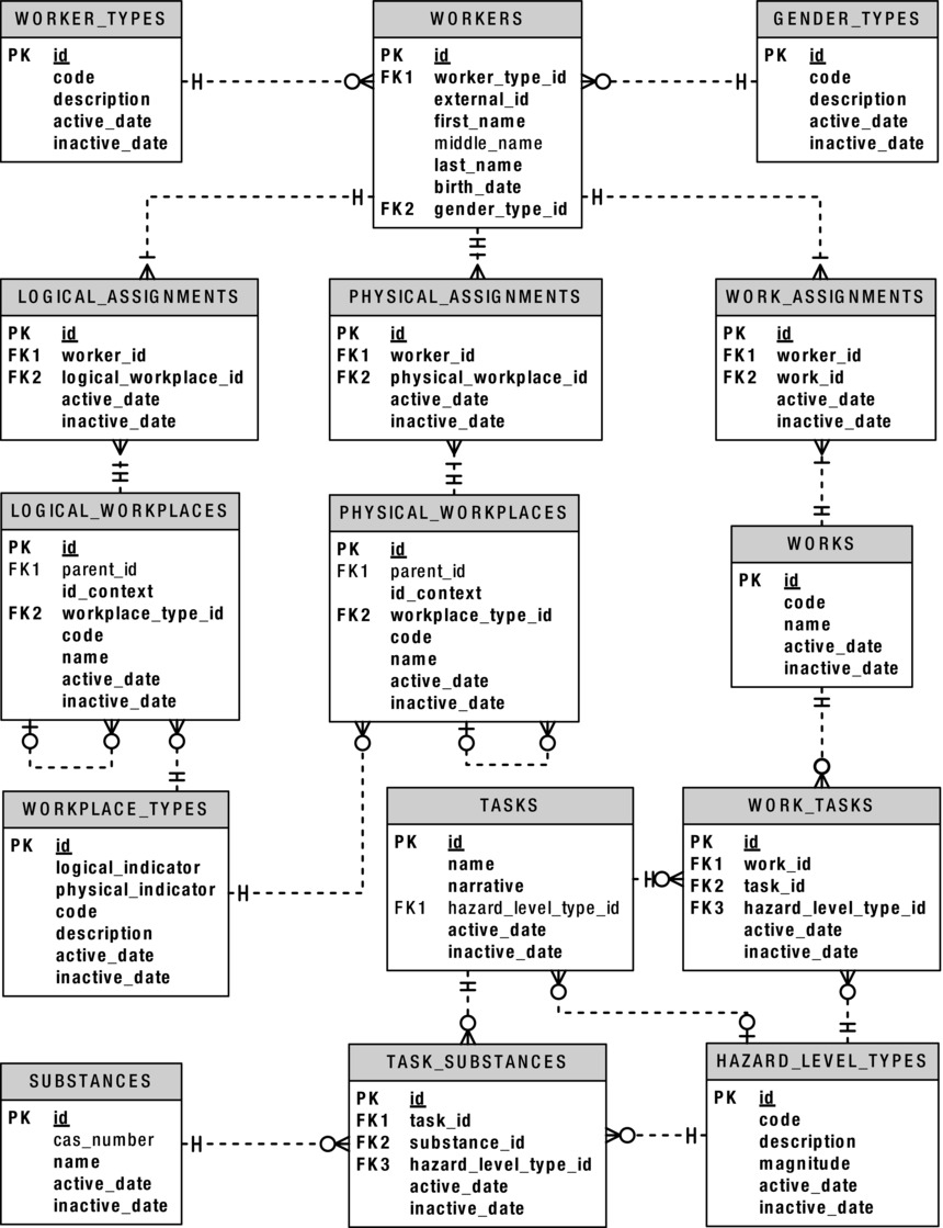
Figure 1-2. VMDI’s IH, OH, and safety demographic subsystem ERD
In order for you to get a better understanding of the ERD, think of each table in the diagram as one of the following:
- Content
- Codes
- Intersections
What do these terms mean?
Think of content as anything your users may actually need to type into the system, which varies greatly. For example, information like a worker’s name and birth date changes a lot from one worker to the next. Since that data is kept in the WORKERS table, think of the WORKERS table as a content table.
Data in the WORKERS table is the kind of information that you’re unlikely to translate into another language should you present the information in a report. I would also classify as content tables the LOGICAL_WORKPLACES, PHYSICAL_WORKPLACES, and WORKS tables, which describe the organization, location, and the job of a worker, respectively. However, you might also think of them as codes.
In order to make the categorization, classification, or typing of data specified in a content table consistent across all entries—for example, workers entered into the WORKERS table—I’ve added some code tables. There are only a limited number of types of workers, and definitely only a limited number of genders, so I’ve added a WORKER_TYPES code table and a GENDER_TYPES code table. Code tables act as the definitive source of categories, classes, types, and so on when specifying codified information in a content table like WORKERS.
Here are some of the reasons that it’s important to use code tables:
- They constrain the values entered into a table to an authoritative list of entries. This improves quality.
- The primary key of a code table is typically an identifier (ID) that is a sequence-generated number with no inherent meaning other than it is the primary key’s value. An ID value is a compact value that can then be stored in the content table to reference the much larger code and description values. This improves performance.
- Storing the sequence-generated ID of a code table in a content table will allow you to later change the code or description values for a particular code without needing to do so in the content table. This improves application maintenance.
- Storing the sequence-generated ID of a code table in a content table will also allow you to later change the code or description for a code on the fly for an internationalized application. This improves flexibility.
Think of the WORKER_TYPES, GENDER_TYPES, WORKPLACE_TYPES, and HAZARD_LEVEL_TYPES tables as code tables. They all have a similar set of behaviors that you will later make accessible with PL/SQL functions and procedures.
Intersections
Think of intersections as a means of documenting history. Understanding that there is a history of information is the single-most portion missing in the analyses of business problems. Most often, a many-to-many relationship table (an intersection) will be created that captures only the “current” relationship between content entities, but there’s always a history, and the history is almost always what’s actually needed to solve the business problem in question.
In the refresher earlier in this chapter, you worked with two tables (or entities) that did not require you to keep a history. However, in the example here, you definitely need to maintain a history of who workers reported to, where they actually did their work, and what they did. Intersections document timelines, as shown in Figure 1-3.
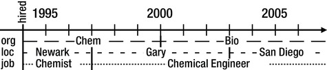
Figure 1-3. An employment timeline
Examining Figure 1-3, you can see that the employee in question has the following history:
- Worked in the Chemicals department from 1994 through 1999, and then in the Biologicals department since (logical assignment)
- Worked at the Newark, New Jersey location from 1994 through 1996, in Gary, Indiana through 2002, and then in sunny San Diego since (physical assignment)
- Worked as a chemist from 1994 through 1996, and then as a chemical engineer since (work assignment)
An intersection table has a beginning and end date for every assignment period. Think of the LOGICAL_ASSIGNMENTS, PHYSICAL_ASSIGNMENTS, and WORK_ASSIGNMENTS tables as history tables that hold an intersection in time between the WORKERS table and the LOGICAL_WORKPLACES, PHYSICAL_WORKPLACES, and WORKS tables, respectively.
Now that you’re familiar with the ERD, you can start creating the tables.
Create a Code Table
Let’s create some code tables. I’ll write the script for the first code table, and then you do the other three. Listing 1-26 is a script to create the WORKER_TYPES code table.
Listing 1-26. DDL for Creating the WORKER_TYPES Code Table, worker_types.tab
01  rem worker_types.tab
02  rem by Donald J. Bales on 2014-10-20
03  rem
04
05  --drop   table WORKER_TYPES;
06  create table WORKER_TYPES (
07  id                             number(38)                     not null,
08  code                           varchar2(30)                   not null,
09  description                    varchar2(80)                   not null,
10  active_date                    date     default SYSDATE       not null,
11  inactive_date                  date     default '31-DEC-9999' not null);
12
13  --drop   sequence WORKER_TYPES_ID;
14  create sequence WORKER_TYPES_ID
15  start with 1;
16
17  alter  table WORKER_TYPES add
18  constraint   WORKER_TYPES_PK
19  primary key ( id )
20  using index;
21
22  alter  table WORKER_TYPES add
23  constraint   WORKER_TYPES_UK
24  unique ( code, active_date )
25  using index;
26
27  execute SYS.DBMS_STATS.gather_table_stats(USER, 'WORKER_TYPES'),
This listing is more complex than the previous ones in this chapter. Here’s the breakdown:
- Lines 1 through 3 document the name of the script, the author, and the date it was written. This is typical—everyone wants to know who to blame.
- Lines 5 and 13 have DROP statements that I’ve commented out. Those were really handy when I was in the iterative development cycle, where I had to edit my script to refine it and then recompile.
- Lines 6 through 11 contain the DDL to create the table WORKER_TYPES.
- Lines 14 and 15 contain the DDL to create WORKER_TYPES_ID, a sequence for the table’s primary key column, id.
- Lines 17 through 20 contain the DDL to alter the table in order to add a primary key constraint.
- Lines 22 through 25 contain the DDL to alter the table in order to add a unique key constraint. This constraint will allow only unique code values in the code table.
Since it’s a code table, I can seed it with some initial values. I’ve written a second script for that, shown in Listing 1-27.
Listing 1-27. DML Script to Populate the WORKER_TYPES Code Table, worker_types.ins
01  rem worker_types.ins
02  rem by Donald J. Bales on 2014-10-20
03  rem
04
05  insert into WORKER_TYPES (
06         id,
07         code,
08         description )
09  values (
10         WORKER_TYPES_ID.nextval,
11         'C',
12         'Contractor' );
13
14  insert into WORKER_TYPES (
15         id,
16         code,
17         description )
18  values (
19         WORKER_TYPES_ID.nextval,
20         'E',
21         'Employee' );
22
23  insert into WORKER_TYPES (
24         id,
25         code,
26         description )
27  values (
28         WORKER_TYPES_ID.nextval,
29         'U',
30         'Unknown' );
31
32  commit;
33
34  execute SYS.DBMS_STATS.gather_table_stats(USER, 'WORKER_TYPES'),
Here’s what’s happening in Listing 1-27:
- In lines 1 through 3, I’ve added the author and written date.
- In lines 5 through 12, 14 through 21, and 23 through 30, I’ve added three DML INSERT VALUES statements in order to add three worker types to the WORKER_TYPES table.
- In lines 10, 19, and 28, I’m allocating a new sequence value from the primary key’s sequence using the pseudo-column .nextval.
- In line 32, I commit the inserts so they are permanently accessible to everyone on the database.
After I execute these two scripts, I can query WORKER_TYPES and get results like this:
SQL> column code          format a4;
SQL> column description   format a13;
SQL> column active_date   format a13;
SQL> column inactive_date format a13;
SQL>
SQL> select *
  2  from   WORKER_TYPES
  3  order by code;

        ID CODE DESCRIPTION   ACTIVE_DATE   INACTIVE_DATE
---------- ---- ------------- ------------- -------------
         1 C    Contractor    07-DEC-14     31-DEC-99
         2 E    Employee      07-DEC-14     31-DEC-99
         3 U    Unknown       07-DEC-14     31-DEC-99
CODING CONVENTIONS
Coding conventions (or standards) are something all professional programmers follow religiously.
SQL Coding Conventions
In the refresher part of this chapter, I capitalized the SQL keywords so it was easy for you to notice them in the syntax statement that followed their use. In practice, I don’t do that. When I code SQL, I follow these simple rules:
- I type table names in all caps, literals in uppercase/lowercase/mixed case as required, and everything else in lowercase. Why? First, since SQL is table-centric, I want table names to stick out like a sore thumb. Second, lowercase is actually easier to read. And finally, lowercase is easier to type, and after 30 years of typing, you’ll know why that’s important.
- I format my code so column names, table names, and parameters in WHERE clauses all line up in nice left-justified columns. That way, the text is easy to scan.
- I name scripts with the same name as the object they are creating, dropping, inserting, updating, and so on, and an appropriate filename extension in order to make the names of the scripts as obvious as possible.
SQL Filename Extension Conventions
The following are the filename extensions I use:
- .tab: Create table
- .alt: Alter table (to add, modify, or drop a column)
- .ndx: Create index
- .pkc: Alter table/add constraint/primary key (usually included in the create table script)
- .fkc: Alter table/add constraint/foreign key (usually included in the create table script)
- .ukc: Alter table/add constraint/unique (usually included in the create table script)
- .drp: Drop table
- .ins: Insert into
- .upd: Update
- .del: Delete from
- .sql: Select from
It’s Your Turn to Create Code Tables
Now that you’ve seen me do it, you should be able to code the scripts to do the same for the GENDER_TYPES, HAZARD_LEVEL_TYPES, and WORKPLACE_TYPES code tables. Code the scripts, saving them with the filenames gender_types.tab, hazard_level_types.tab, and workplace_types.tab, respectively. Then execute each script. You can see my solutions to these scripts in the book’s source code directory for Chapter 1. Now let’s move on to creating content tables.
Create a Content Table
This time, let’s create some content tables. I’ll write the first two scripts, and then you do the rest. Listing 1-28 is a script to create the WORKERS table.
Listing 1-28. DDL to Create the WORKERS Table, workers.tab
01  rem workers.tab
02  rem by Donald J. Bales on 2014-10-20
03  rem
04
05  --drop   table WORKERS;
06  create table WORKERS (
07  id                             number(38)                     not null,
08  worker_type_id                 number(38)                     not null,
09  external_id                    varchar2(30)                   not null,
10  first_name                     varchar2(30)                   not null,
11  middle_name                    varchar2(30),
12  last_name                      varchar2(30)                   not null,
13  name                           varchar2(100)                  not null,
14  birth_date                     date                           not null,
15  gender_type_id                 number                         not null );
16
17  --drop   sequence WORKERS_ID;
18  create sequence WORKERS_ID
19  start with 1;
20
21  --drop   sequence EXTERNAL_ID_SEQ;
22  create sequence EXTERNAL_ID_SEQ
23  start with 100000000 order;
24
25  alter  table WORKERS add
26  constraint   WORKERS_PK
27  primary key ( id )
28  using index;
29
30  alter  table WORKERS add
31  constraint   WORKERS_UK1
32  unique ( external_id )
33  using index;
34
35  alter  table WORKERS add
36  constraint   WORKERS_UK2
37  unique (
38  name,
39  birth_date,
40  gender_type_id )
41  using index;
42
43  alter  table WORKERS add
44  constraint   WORKERS_FK1
45  foreign key   ( worker_type_id )
46  references   WORKER_TYPES ( id );
47
48  alter  table WORKERS add
49  constraint   WORKERS_FK2
50  foreign key   ( gender_type_id )
51  references   GENDER_TYPES ( id );
52
53  execute SYS.DBMS_STATS.gather_table_stats(USER, 'WORKERS'),
Looks familiar, doesn’t it? It looks a lot like the code table scripts you created earlier. The exceptions are lines 43 through 46 and 48 through 51, where I’ve added DDL to create two foreign key constraints. The first foreign key creates an integrity constraint between the code table WORKER_TYPES, while the second does the same for code table GENDER_TYPES. These constraints will prevent anyone from deleting a code that is in use by the WORKERS table.
Listing 1-29 shows the code to create the LOGICAL_WORKPLACES table. I’m showing you this listing because this table has some interesting new columns: parent_id and id_context.
Listing 1-29. DDL to Create the LOGICAL_WORKPLACES Table, logical_workplaces.tab
01  rem logical_workplaces.tab
02  rem by Donald J. Bales on 2014-10-20
03  rem
04
05  --drop   table LOGICAL_WORKPLACES;
06  create table LOGICAL_WORKPLACES (
07  id                             number(38)                     not null,
08  parent_id                      number(38),
09  id_context                     varchar2(100)                  not null,
10  workplace_type_id              number                         not null,
11  code                           varchar2(30)                   not null,
12  name                           varchar2(80)                   not null,
13  active_date                    date     default SYSDATE       not null,
14  inactive_date                  date     default '31-DEC-9999' not null );
15
16  --drop   sequence LOGICAL_WORKPLACES_ID;
17  create sequence LOGICAL_WORKPLACES_ID
18  start with 1;
19
20  alter  table LOGICAL_WORKPLACES add
21  constraint   LOGICAL_WORKPLACES_PK
22  primary key (
23  id )
24  using index;
25
26  alter  table LOGICAL_WORKPLACES add
27  constraint   LOGICAL_WORKPLACES_UK1
28  unique (
29  id_context )
30  using index;
31
32  alter  table LOGICAL_WORKPLACES add
33  constraint   LOGICAL_WORKPLACES_UK2
34  unique (
35  code,
36  name,
37  active_date )
38  using index;
39
40  alter  table LOGICAL_WORKPLACES add
41  constraint   LOGICAL_WORKPLACES_FK1
42  foreign key              ( parent_id )
43  references   LOGICAL_WORKPLACES ( id );
44
45  alter  table LOGICAL_WORKPLACES add
46  constraint   LOGICAL_WORKPLACES_FK2
47  foreign key   ( workplace_type_id )
48  references   WORKPLACE_TYPES ( id );
49
50  execute SYS.DBMS_STATS.gather_table_stats(USER, 'LOGICAL_WORKPLACES'),
A logical workplace like a department may belong to a business unit, while its business unit may belong to a company. The parent_id column allows you to store the id of a department’s parent business unit with the department, so you can document the organization hierarchy. With this information, you can present an organization chart, find everyone in a business unit, and so on.
The id_context column is a convenience or performance column for the mechanics of querying the database. You are going to write a PL/SQL function that will create an ID context string for this column. The ID context string will list all of the parent IDs, plus the logical workplace ID of the current row, separated by a known character, such as a period (.)—for example, 1.13.14. This will greatly improve the performance of any LIKE queries against the hierarchy of the organizations in the table.
It’s Your Turn to Create Content Tables
Now that you’ve seen me do it, you should be able to code the scripts to do the same for the PHYSICAL_WORKPLACES , TASKS, and WORKS tables. So code the scripts, saving them with the filenames physical_workplaces.tab, tasks.tab, and works.tab, respectively. Then execute each script. You can view my solutions to these scripts in the book’s source code directory for Chapter 1.
Now let’s move on to creating intersection tables.
Create an Intersection Table
It’s time to create some intersection tables. I’ll write the first script, and then you write the rest. Listing 1-30 is a script to create the LOGICAL_ASSIGNMENTS table.
Listing 1-30. DDL to Create the LOGICAL_ASSIGNMENTS Table, logical_assignments.tab
01  rem logical_assignments.tab
02  rem by Donald J. Bales on 2014-10-20
03  rem
04
05  --drop   table LOGICAL_ASSIGNMENTS;
06  create table LOGICAL_ASSIGNMENTS (
07  id                             number(38)                     not null,
08  worker_id                      number(38)                     not null,
09  logical_workplace_id           number(38)                     not null,
10  active_date                    date     default SYSDATE       not null,
11  inactive_date                  date     default '31-DEC-9999' not null );
12
13  --drop   sequence LOGICAL_ASSIGNMENTS_ID;
14  create sequence LOGICAL_ASSIGNMENTS_ID
15  start with 1;
16
17  alter  table LOGICAL_ASSIGNMENTS add
18  constraint   LOGICAL_ASSIGNMENTS_PK
19  primary key ( id )
20  using index;
21
22  alter  table LOGICAL_ASSIGNMENTS add
23  constraint   LOGICAL_ASSIGNMENTS_UK
24  unique (
25  worker_id,
26  active_date )
27  using index;
28
29  alter  table LOGICAL_ASSIGNMENTS add
30  constraint   LOGICAL_ASSIGNMENTS_FK1
31  foreign key   ( worker_id )
32  references   WORKERS ( id );
33
34  alter  table LOGICAL_ASSIGNMENTS add
35  constraint   LOGICAL_ASSIGNMENTS_FK2
36  foreign key   ( logical_workplace_id )
37  references   LOGICAL_WORKPLACES ( id );
38
39  execute SYS.DBMS_STATS.gather_table_stats(USER, 'LOGICAL_ASSIGNMENTS'),
I know; you don’t even need me to explain it anymore. I just wanted to make sure you have a nice pattern to mimic.
It’s Your Turn to Create Intersection Tables
Just do it! Create tables PHYSICAL_ASSIGNMENTS, WORK_ASSIGNMENTS, and WORK_TASKS. Code your scripts with file names physical_assignments.tab, work_assignments.tab, and work_tasks.tab. Then execute your scripts.
Summary
By now you should have a fairly complete set of sample tables that you can work with when programming in PL/SQL. You’ve reviewed the basics of relational SQL, and then put that to work to create your working example. If you had any trouble with the SQL used so far, I sincerely encourage you to get some supplemental materials and/or training in order to improve your SQL skills. You’ve heard the old adage, “A chain is only as strong as its weakest link,” haven’t you?
So you think your SQL is up to the task of programming in PL/SQL? Well, let’s get started!