
This chapter is not required in order to understand other chapters in this book. While we introduce some new techniques, what you primarily find here is one entire dashboard sample ready to be modified to suit your needs.
Just what does this sampler do? It takes the applications we used in the preceding chapter and presents them in an engaging, interactive format. It is important to keep in mind that while we often present these applications with a graphical output, any R process can be done to these data. The goal is to allow information consumers the capability to naturally interact with live data, whether those consumers are research reviewers, next-level directors, or board members.
Similarly to the last chapter, we introduce this on Windows inside RStudio (RStudio Team, 2015). We provide both a framework to understand this dashboard, as well as some pro tips. It is important to see this sampler as a creativity incubator of sorts. It is our hope that you see something you like, and more vitally, realize just how you can best showcase your data.
We will start with the underlying structure of a dashboard.
A Dashboard’s Bones
Recall our littlest shiny (Chang, Cheng, Allaire, Xie, and McPherson, 2016) application from the preceding chapter:
library(shiny)# Define user interfaceui <- shinyUI(fluidPage())# Define serverserver <- shinyServer(function(input, output) {})# Run the applicationshinyApp(ui = ui, server = server)
This code was good to look at from the beginning, because it highlights how all Shiny applications comprise a user interface, and a server side where the R code logic lives—and these are both run as an R process themselves (possibly on a cloud server). All we intend to add to this structure is some code on the user-interface side. This should make sense, because a dashboard is more about user interface than any new code logic. The goal is to make analytics and statistical inferences readily available to users. There is a new library to install for this, but it is just one, shinydashboard (Chang, 2015). From the command line of RStudio, go ahead and run the following code:
install.packages("shinydashboard") With this new package installed, we may now take a look at the littlest Shiny dashboard application. Dashboards include a header, a sidebar with various menu items, and the main body in which the different objects of the applications exist. Compare and contrast this dashboard code layout to the single application code. The two versions are almost the same. After the code, see what they generate in Figure 14-1.
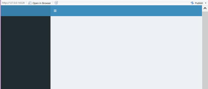
Figure 14-1. The littlest Shiny dashboard is quite empty
library(shiny)library(shinydashboard)# Define user interfaceui <- dashboardPage(dashboardHeader(),dashboardSidebar(),dashboardBody())# Define serverserver <- shinyServer(function(input, output) {})# Run the applicationshinyApp(ui = ui, server = server)
As you can see in the preceding code, we have three functions: dashboardHeader(), dashboardSidebar(), and dashboardBody(). These provide a nice structure for our dashboard. These all reside inside dashboardPage() as the first three of five formal arguments for the page function. The final two formals include title (which defaults to NULL) as well as skin (which takes on one of blue, black, purple, green, red, or yellow color). As you can see for yourself with the formals(dashboardPage) command, the page function is indeed simple enough. The title argument controls the heading in the browser itself (or on the browser tab, if multiple tabs are open in most popular browsers). The skin color options control the overall color palette of the dashboard. Now, the first three formals are functions in their own right and become quite complex. Nevertheless, we will get to all three in turn.
Dashboard Header
The dashboardHeader() function also takes a title formal that adds user-defined text into the header area as well as a titleWidth argument controlling the width of that text. The header also accepts several other Shiny user-interface-style functions to control page navigation along with a handful of more specialized functions that allow for more interactive navigation. In this chapter, and indeed this book, we essentially ignore these functions to promote shiny and shinydashboard as ways of serving already familiar R code to data consumers rather than learning too many new features all at once. In fact, the last formal we mention for this function is disable, which defaults to FALSE and on TRUE hides the header entirely. In our sampler, we will preserve the header in a mostly tabula rasa state.
Dashboard Sidebar
Moving on to the dashboardSidebar() function , the only explicitly called-out formals are again a disable option along with a width argument. However, there are more functions possible here beyond the called-out ones. The first thing to know is that any of the user-interface functions from shiny works in the sidebar. Thus, if it makes sense to place a slider bar or drop-down input functions in your menu, that is possible. There are, however, some functions unique to the dashboard library that make sense to place inside the sidebar area.
The first of these is the sidebarMenu() function . Much like dashboardSidebar() itself, this function primarily takes other inputs and handles the organization of them in an efficient fashion. Of particular note is the menuItem() function , which is called from inside sidebarMenu(). In this sampler, we house each of the applications created in the previous chapter in their own call to menuItem(). As you can see in the following code, this function has several formals:
formals(menuItem)$text$...$iconNULL$badgeLabelNULL$badgeColor[1] "green"$tabNameNULL$hrefNULL$newtab[1] TRUE$selectedNULL
In the preceding function and formal arguments, the text takes a text string in quotes that provides the text information or link name for that particular item on the menu. The icon formal is given a name for a Font-Awesome icon. We provide a link to the online library, showcasing all possible icon choices in the references section of this chapter. We may also switch to a different icon library; we save such explorations for you. The badgelabel call puts an inline badge on the far right of the sidebar, which fits a short bit of text. Badges do a good job of calling viewers’ attention to a particular menu item and, consequently, to the underlying application. Many of these formals are somewhat optional; however, there must be either a tabName linked to a related tabItem() in the dashboard’s body or there must be a URL given to the href command. If a URL is given rather than a tabName, then newtab can be changed from a default of TRUE to FALSE should you wish your viewer to leave your site when visiting that page. Finally, it is possible to force the default to a particular tab, away from the first menuItem(), by setting selected to TRUE.
As we turn our attention to the main body of our dashboard, we remind you that the sidebar can also receive any Shiny function—such as the img() function which points to an image that must be contained in a folder named www inside your dashboard application’s folder. We show a code snippet (which should not be run yet) of our sampler’s menu along with the result in Figure 14-2. The names of the first three menu items should be familiar from the prior chapter.

Figure 14-2. The result of some sidebarMenu() and menuItem() functions
sidebarMenu(menuItem("Pie Charts!", tabName = "PieChart_Time", icon = icon("pie-chart")),menuItem("Use a Slider", tabName = "slider_time", icon = icon("sliders"), badgeLabel = "New"),menuItem("Upload a Histogram File", tabName = "Upload_hist", icon = icon("bar-chart")),menuItem("Labour Data Dates", tabName = "labour", icon = icon("cloud-download"), badgeLabel = "Live"))
Dashboard Body
As you can see in the preceding code, each menu item has tabName. We will now discuss the code inside the dashboardBody() function that will catch that tabName. Take a look at the little, although not the littlest, Shiny dashboard in the following code and Figure 14-3, and then we will walk through the new lines.

Figure 14-3. A dashboard with a menuItem() in the sidebar and a tabItem() in the body. Notice the matching First.
library(shiny)library(shinydashboard)# Define user interfaceui <- dashboardPage(dashboardHeader(),dashboardSidebar(sidebarMenu(menuItem("Demo", tabName = "First"))),dashboardBody(tabItems(tabItem(tabName = "First", "test"))),skin = "yellow")# Define serverserver <- shinyServer(function(input, output) {})# Run the applicationshinyApp(ui = ui, server = server)
Many items might be placed inside the body of our dashboard. However, if we want to use the tabs that we coded back in the sidebar section, we do a general call to tabItems(). This function takes no arguments except individual tabItem() function calls; each of those tabItems() needs to have a unique tabName matching a unique tabName from the sidebarMenu().
What goes inside each tabItem()? Well, just as in Shiny, there is a benefit to making the layout fluid enough that your dashboard can cope with various-sized browser windows. Thus, the common function fluidRow() makes a reappearance. Recall that fluidRow() is set up to have a row width of at most 12. Remembering that fact, keep a sharp lookout at the default widths for each of the three box objects we discuss to fill those rows. Now, there are more than these three objects; again, our goal is to get you quickly to the point where you may serve your data via the cloud to your users or stakeholders.
The most basic input element to go in a row is box(). Inside this function, we place any of the application code we used in the preceding chapter to either solicit input from users or to output reactive content. However, box() also takes nine specific arguments. Naturally, each box() may take a title value, a user-defined text string that should succinctly describe the contents of the box or the action required. At the bottom of the box, there is a footer, which may also take a text string. Boxes also have a status that may be set to take on values of primary, success, info, warning, or danger. Each of those status values has an associated color that is part of the default Cascading Style Sheets structure that makes shinydashboard look rather pretty. The colors are fairly consistent, although they may have some variance depending on which color you selected for the whole dashboard. The default value for solidHeader is FALSE, although this, of course, may be changed to TRUE. The positive choice simply enhances the color of the status to become a narrow banner background to the title text. Should you wish the main area of your box to have a specific color, background can be set from approximately 15 valid colo choices. Any input code and any output code lives on top of that background, as the name suggests. The default width for a box is 6, so two boxes fill up a row unless you take steps to narrow them. Failure to keep the total fluidRow() width of 12 in mind can lead to some odd layouts. Box height can also be set to a fixed height. This can be helpful if you require very even rows. Finally, boxes are collapsible and may be already collapsed, although both options default to FALSE. Figure 14-4 shows some results of these various settings.

Figure 14-4. A familiar application in two boxes with various options—see Complete Sampler Code for details
Another type of box is valueBox(), which takes six formal arguments. The first is value, which is usually a short text string or value, as shown in Figure 14-5. The valueBox() also takes a subtitle argument, which is again a text string. You can choose an icon, although the default value is NULL. These boxes come with a default color of aqua and are rather short with a default width of only 4. Finally, valueBox() also takes a value for href, which defaults to NULL. We show the code we used in our sampler’s value box here:

Figure 14-5. Sample valueBox() showing the number of days of data that were pulled live from a website
valueBox(endYear-startYear, "Days of Data", icon = icon("calendar"))We finish out our discussion of the dashboardBody() boxes with a box similar to the valueBox(): the infoBox(). This box comes with a title that takes a text string, a value to highlight and display in the box, optional subtitle text, and a default icon of a bar chart. It also features defaults for color of aqua, width 4, and a NULL href. What is different is that the icon is smaller, and there is a fill option, which is usually FALSE, that can change the way the background color displays. We do not show this box, but it does look quite similar to the small box in Figure 14-5. In our experience, these boxes are not significantly different other than in their appearance.
Dashboard in the Cloud
We do want to serve this dashboard into our cloud instance, and this is a slightly more complex set of code. Again, we created this in a standard Shiny folder by using RStudio, so it comes in its own file. The file structure on Windows looks like Figure 14-6. There are three files in our shinydashboard_cloud folder. Note the www folder, which hosts our sampler’s image, followed by the app.R file, which holds our entire Shiny application as well as our CSV file.

Figure 14-6. The file structure for shinydashboard_cloud
We use WinSCP to upload our files and folders to our Ubuntu cloud instance, as shown in Figure 14-7.

Figure 14-7. WinSCP upload folder view
Logging into PuTTY, we do have some work to do. Our sampler uses some new libraries, and, of course, the file needs to be moved from our user’s folder to where the Shiny server expects it to live. For brevity, we install only the packages we have not yet installed on our cloud instance.
The first of the new packages is XML (Lang, D. et al., 2016), and this package provides the ability to read in an HTML table live from the Web. Various government and nonprofit agencies store data in such tables for easy access by the public. We also install the zoo package (Zeileis and Grothendieck, 2005), which provides convenient functions for time series. Already familiar packages are ggplot2 (Wickham, 2009) and data.table (Dowle, Srinivasan, Short, and Lianoglou, 2015), which handle graphical plotting and provide a more advanced data frame structure.
The following commands run one at a time on our instance installation for all users’ five new libraries and then copy the files so they are accessible via a browser. We also install some software onto Ubuntu that is required to allow the XML package to run. For readability, we group some of the following commands together. They should be run one line at a time in PuTTY, and some text prints to the screen after each command.
sudo su - -c "R -e "install.packages('shinydashboard', repos='https://cran.rstudio.com/')""sudo apt-get install libcurl4-openssl-dev libxml2-devsudo su - -c "R -e "install.packages('XML', repos='https://cran.rstudio.com/')""sudo su - -c "R -e "install.packages('zoo', repos='https://cran.rstudio.com/')""sudo su - -c "R -e "install.packages('data.table', repos='https://cran.rstudio.com/')""sudo su - -c "R -e "install.packages('ggplot2', repos='https://cran.rstudio.com/')""sudo cp -R ∼/shinydashboard_cloud /srv/shiny-server/
This completes our work with Shiny and the Shiny dashboard. Your dashboard should be live at http://Your.Instance.IP.Address:3838/shinydashboard_cloud/ and viewable from your web browser. We have a few more comments to make before we close out the chapter.
First, we highly suggest that you visit the Apress site for this textbook and download the code bundle for this chapter. It contains the complete, working files and folders shown in Figure 14-6 and uploaded in Figure 14-7. There is no need to manually type all this code to see whether a dashboard might be something you would like to have.
Second, we have in no way throughout this chapter given our full sample code. We saved that for the end to keep it all in a single, cohesive whole and to focus your attention on the specific structure you want to be looking for in that sampler code.
Third, we remind you that if you have followed our security-minded advice about inbound policy settings on the AWS servers, you may need to change those settings to allow more people than just yourself to view your final dashboard project. Remember, the setting you need to change on the inbound side is to allow port 3838 to be accessed from 0.0.0.0/0, which is the entire Internet. Keep in mind that the entire Internet is then able to access your dashboard. If you have sensitive data, or even information that just does not need to be out and about, please consider partnering with an IT professional or at least an IT power user.
Finally, we hope you enjoyed this chapter and the results as much as we have. Be sure to explore the links in the “References” section. You will find valuable information ranging from additional functions, a whole list of icons, a whole second icon library, and the very latest in shiny and shinydashboard package information. These packages are updating fairly regularly, and new features can often provide awesome results.
Complete Sampler Code
library(shiny)library(shinydashboard)library(XML)library(zoo)library(data.table)library(ggplot2)#this code will run just once each time a session is instantiated - there may be multiple viewers in the same session.slider_data<-read.csv("slider_data.csv", header = TRUE, sep = ",")Phase1 <- slider_data[,2]Phase2 <- slider_data[,3]Phase3 <- slider_data[,4]Phase4 <- slider_data[,5]bls <-readHTMLTable("http://data.bls.gov/timeseries/LAUMT484702000000006?data_tool=XGtable", stringsAsFactors = FALSE)bls <- as.data.table(bls[[2]])bls[, names(bls):= lapply(.SD, function(x) {x <- gsub("\(.*\)", "", x)type.convert(x)})]setnames(bls,names(bls), gsub("\s","",names(bls)))bls[, Date := as.Date(paste0(Year, "-", Period, "-01"), format="%Y-%b-%d")]startYear<-min(bls$Date)endYear<-max(bls$Date)### We now define the user interface to be a dashboard pageui <- dashboardPage(dashboardHeader(title = "Advanced R"),dashboardSidebar(img(src = "egl_logo_full_3448x678.png", height = 43, width = 216),sidebarMenu(menuItem("Pie Charts!", tabName = "PieChart_Time", icon = icon("pie-chart")),menuItem("Use a Slider", tabName = "slider_time", icon = icon("sliders"),badgeLabel = "New"),menuItem("Upload a Histogram File", tabName = "Upload_hist", icon = icon("bar-chart")),menuItem("Labour Data Dates", tabName = "labour", icon = icon("cloud-download"),badgeLabel = "Live")) ),dashboardBody(tabItems(# PieChart_Time Content which should be familiartabItem(tabName = "PieChart_Time",fluidRow(box( title = "PieChart_Time", status = "warning",numericInput("pie", "Percent of Pie Chart", min = 0, max = 100, value = 50),textInput("pietext", "Text Input", value = "Default Title", placeholder = "Enter Your Title Here"),checkboxInput("pieChoice"," I want a Pie Chart instead.", value = FALSE)),box( title = "Graphical Output", solidHeader = TRUE, status = "warning",plotOutput("piePlot")))),# Slider Tab Content which should be familiartabItem(tabName = "slider_time",h2("Training Programme Results"),box( title = "Control the Academic Year", status = "primary", solidHeader = TRUE,sliderInput("ayear", "Academic Year:", min = 2014, max = 2017, value = 2014, step = 1,animate = animationOptions(interval=600, loop=T))),box(plotOutput("barPlot"))),##Histogram from an Uploaded CSV which should be familiartabItem( tabName = "Upload_hist",fluidRow(box( title = "File Input",# Copy the line below to make a file upload managerfileInput("file", label = h3("Histogram Data File input"),multiple = FALSE)),box( title = "Data from file input", collapsible = TRUE,tableOutput("tabledf"))),fluidRow(box(tableOutput("tabledf2")),box( background = "blue",plotOutput("histPlot1")))),###This Labour plot Tab is new and uses data pulled fresh from the web each time an R instance ##is created.tabItem(tabName = "labour",fluidRow(box( dateRangeInput("labourDates", min = startYear,max = endYear,start = startYear, end = endYear,label = h3("Date range")),selectInput("labourYvalue", label = h3("Select box"),choices = list("LaborForce" = 3,"Employement" = 4,"Unemployement" = 5),selected = 3),radioButtons("labourRadio", "Rolling Average", selected = FALSE,choices = list("Yes"=TRUE, "No"=FALSE))),box(title = "Test", plotOutput("labourPlot"))),fluidRow( valueBox(endYear-startYear, "Days of Data", icon = icon("calendar")))))),title = "Dashboard Sampler", skin = "yellow")#### Define server logic required to draw a histogram#####server <- shinyServer(function(input, output) {output$piePlot <- renderPlot({# generate Pie chart ratios based on input$pie from usery <- c(input$pie, 100-input$pie)# draw the pie chart or bar plot with the specified ratio and labelif(input$pieChoice == FALSE){barplot(y, ylim = c(0,100), names.arg = c(input$pietext, paste0("Complement of ", input$pietext)))}else{pie(y, labels = c(input$pietext, paste0("Complement of ", input$pietext)))}})output$barPlot <- renderPlot({# Count values in each phase that match the correct date.cap<-input$ayear*100x <- c(sum(Phase1<cap), sum(Phase2<cap), sum(Phase3<cap), sum(Phase4<cap))# draw the bar plot for the correct year.barplot(x,names.arg = c("Phase I", "Phase II", "Phase III", "Fellows"),col = c("deeppink1","deeppink2","deeppink3","deeppink4"), ylim=c(0,50))})####Here is where the input of a file happensoutput$tabledf<-renderTable({ input$file })histData<-reactive({file1<-input$fileread.csv(file1$datapath,header=TRUE ,sep = ",")})output$tabledf2<-renderTable({ histData() })output$histPlot1<-renderPlot({ hist(as.numeric(histData()$X1)) })##############labour plot####################output$labourPlot<-renderPlot({xlow<-input$labourDates[1]xhigh<-input$labourDates[2]blsSub <- bls[Date<=xhigh&Date>=xlow]yValue <- names(blsSub)[as.numeric(input$labourYvalue)]if(input$labourRadio == TRUE && nrow(blsSub)>=4){ blsSub[,(yValue):=rollmean(get(yValue), k=3, na.pad = TRUE)] }ggplot(data = blsSub, mapping = aes_string("Date", yValue)) +geom_line()+xlab("Years & Months")+ylab("People")+xlim(xlow, xhigh)+ggtitle(yValue)+scale_x_date(date_labels = "%b %y")}) })# Run the applicationshinyApp(ui = ui, server = server)