
In the preceding chapters, you saw how Shiny delivers interactive environments based on dynamic data. Dynamic reports and the live dashboards have many similarities. On the other hand, this chapter, because the reports end up as PDFs, is less interactive. Reports are a fact of life in many fields, and stakeholders tend to require snapshots in time rather than fully interactive environments. Through the knitr and rmarkdown packages, we create documents (for example, PDF, HTML, or Microsoft Word) based on data input. For regular reports that build on continuously changing data, yet that have the same structure overall, this is a great time-saver.
The rmarkdown package (Xie, 2015) adds the capability to embed R processes into such documents, allowing one-click analytics that are beautifully formatted using a variety of styles. The LaTeX interface achieves almost any formatting required, although there are options besides PDF. From boardroom reports on enrollment based on live pulls from a student information system database, to strategic plan action-sheets drawn from key performance indicators, dynamic reports work best when variable input needs shaping into standardized output. This is also facilitated via knitr and formatR packages (Xie, 2015).
Additionally, in this chapter, we use the evaluate package (Wickham, 2016) and tufte package (Xie, 2016). These packages allow us to organize the layout and format of our date more elegantly. We also use the ltm package (Rizopoulos, 2006) for the psychometric tests.
Our goals for this chapter are to enhance our software environment both on our local and cloud machines to allow the dynamic documents to compile, explore the structure of standalone rmarkdown, develop a Shiny page that allows a user to upload data and then download a PDF report, and finally to push this all to our cloud instance. We start with needed software.
Needed Software
We already have a great deal of the software needed, namely R, the Shiny packages (Chang, Cheng, Allaire, Xie, and McPherson, 2016), PuTTY, and our cloud instance on Ubuntu. We need a handful of new packages installed—both on the local machine as well as the cloud server.
Local Machine
First, in your R console, it is important to run the following code independent of any R file:
install.packages("rmarkdown")install.packages("tufte")install.packages("knitr")install.packages("evaluate")install.packages("ltm")install.packages("formatR")Dynamic documentlocal machine
After those packages install, we turn our attention to installing MiKTeX (Schenk, 2009), which allows the creation of PDF files. A brief visit to the MiKTeX site ( http://miktex.org/download ) allows you to obtain either the recommended basic installer (which is 32-bit) or the other basic installer (which is 64-bit). We use the 64-bit version for our systems, although in this chapter there is not likely to be a major difference between the versions. After download, accept all the defaults during installation. After installation, there may be updates to the MiKTeX package. To perform these updates, go to your start files. In a folder titled MiKTeX, you’ll find an option for Update near the end. Follow the default options and then select all packages to update to the latest. While not required, we do recommend a restart after this installation.
Cloud Instance
Using PuTTY, access your cloud instance console. We need to run each line of code that follows individually at the console. Recall from an earlier chapter that these install the packages for all users of that server, not just your user. This is key to allow the Shiny server access to the correct packages.
sudo su - -c "R -e "install.packages('rmarkdown', repos = 'http://cran.rstudio.com/')""sudo su - -c "R -e "install.packages('tufte', repos = 'http://cran.rstudio.com/')""sudo su - -c "R -e "install.packages('knitr', repos = 'http://cran.rstudio.com/')""sudo su - -c "R -e "install.packages('ltm', repos = 'http://cran.rstudio.com/')""sudo su - -c "R -e "install.packages('formatR', repos = 'http://cran.rstudio.com/')""sudo su - -c "R -e "install.packages('data.table', repos = 'http://cran.rstudio.com/')""
The preceding code does not take very long. However, installing texlive (the Ubuntu solution for LaTeX used instead of MiKTeX), may take some time. It also demands a fair bit of disk space, so be sure you have room. In our trials, the full version is required.
sudo apt-get install texlive-full After this, we recommend a sudo reboot to restart your cloud instance. This is a good place to do that and then close PuTTY for a bit. While your server restarts, you may use your local machine to explore dynamic documents.
Dynamic Documents
It is not required to link dynamic documents to the Internet in any way. Indeed, most reports may be internal. Inside RStudio, selecting File ➤ New File ➤ R Markdown opens a wizard. Notice that there are options for documents (for example, HTML, PDF, or Word) as well as presentations (for example, HTML or PDF). A title is customary, as is listing the author(s). Of course, RStudio is not required; creating a new file in R with the .Rmd suffix suffices.
We intend to create a hybrid approach to this introduction to dynamic documents. That is, we first give a straightforward and informative example of what such code looks like, and then we follow up with a more in-depth analysis of each piece of that code. We start with a new file titled ch15_html.Rmdand fill it with the following code:
---title: "ch15_html"author: "Matt & Joshua Wiley"date: "18 September 2016"output: html_document---```{r echo=FALSE}##notice the 'echo=FALSE'##it means the following code will never make it to our knited htmllibrary(data.table)diris <- as.data.table(iris)##it is still run, however, so we do have access to it.```#This is the top-level header; it is not a comment.This is plain text that is not code.If we wish *italics* or **bold**, we can easily add those to these documents. Of course, we may need to mention `rmarkdown` is the package used, and inline code is nice for that. If mathematics are required, then perhaps x∼1∼^2^ + x∼2∼^2^ = 1 is wanted.##calling out mathematics with a header 2On the other hand, we may need the mathematics called out explicitly, in which case $x^{2} + y^{2}= pi$ is the way to make that happen.###I like strikeouts; I am less clear about level 3 headers.I often find when writing reports that I want to say something is ∼∼absolutely foolish∼∼ obviously relevant to key stakeholders.######If you ever write something that needs Header 6Then I believe, as this unordered list suggests:* You need to embrace less order starting now- Have you considered other careers?```{r echo=FALSE}summary(diris)```However, notice that one can include both the code and the console output:```{r}hist(diris$Sepal.Length)```
The results of knitting the preceding code are shown in Figure 15-1.

Figure 15-1. The HTML output of a simple dynamic document
As you can imagine, it is the summary data or the graph that is easily regenerated based on any input. In fact, one of the authors uses dynamic documents to create case studies (and a case study key) for students in an introductory statistics course. It is easy enough to generate pseudorandom data with different seeds that allow each student to have a unique data set (and several topics). It also allows for solution keys for fast marking.
Now that you have an overview of Rmarkdown, let’s explore the previous code in sensible blocks. The first block is YAML, which stands for Yet Another Markup Language or possibly the recursively defined YAML Ain’t Markup Language (YAML, 2016) header. At its simplest, it may contain only information about the title, author, date, and the output type. Here, for this document, we selected html_document. However, as stated previously, there are more options such as pdf_document, word_document, odt_document, rtf_document, and beamer_presentation (to name a few—there are in fact more). These types create, respectively, HTML pages, PDFs, Microsoft Word files, OpenDocument or rich text, and Beamer PDF slides. Both Beamer and PDFs require the MiKTeX installation we did earlier. To change the type of document compiled, simply change the output! It is worth noting that the first time you use MiKTeX, it may take longer to compile, as there may need to be a package or two installed behind the scenes. This does not take any user intervention; it simply takes time. It is also worth noting that if you use beamer_presentation, then what can and cannot fit on one slide needs to be considered. In that case, a carriage return followed by ----, followed by another carriage return, signals new slides in your deck.
---title: "ch15_html"author: "Matt & Joshua Wiley"date: "18 September 2016"output: html_document---
Headers can, be more complex than this. R code can be injected inline, using `r code goes here` formatting. Thus, we could change the date to be more dynamic by swapping out date: "18 September 2016" for date: "`r Sys.Date()`" in our code. Dozens of render options work with the YAML header, and wiser heads than ours have created templates that use variants of those headers as well as set several nice options. As in Shiny, there is a nearly limitless ability to customize precisely how a document outputs and displays.
The next region of our markdown code is a code chunk. Code chunks start with ```{r } and end with ```. Between those lives your code. Now, inside the {r } there are several useful options. If you have part of your code that is intensive to create and mostly static, you may want to set cache = TRUE instead of the default FALSE. This stores the results. We use echo=FALSE often, which prevents the code itself, yet not the results of that code, from displaying. Notice that in the first chunk that follows, there is no sign in our final document that the code ran. However, the second chunk still shows the results of summary(diris).
```{r echo=FALSE}library(data.table)diris <- as.data.table(iris)``````{r echo=FALSE}summary(diris)```
For code chunks that involve plots or figures, there are many options too. The fig.align option may be set to right, centre, or left. There are height and width settings for plots with fig.height or fig.width that default to inches.
```{r fig.align="right"}hist(diris$Sepal.Length)```
Finally, there is the text itself, which we do not repeat here because that is of less interest. We do note that code can be written inline as well as just as in the header. You’ll see that this option becomes very useful later, when we want to provide different narrative text depending on our computation results.
Dynamic Documents and Shiny
We turn our attention now to providing not only a dynamic document but one that others may control via their dynamic input. What we build is a simple Shiny environment that allows for a user to upload a CSV file with quiz score data for students. The data is coded as follows: the columns represent specific questions on the quiz; the rows represent individual students; and the quiz is multiple choice, with 1 coded in for correct responses, and 0 coded in for incorrect options.
As in the preceding section, we look at all our code for each of the three files it takes to make this work. Then, we break that code down line by line. For readers already comfortable with Shiny, please feel free to skip to the last portion. We build this code in a folder named Chapter15. Later, when we upload to our Ubuntu server, we upload that entire folder.
server.R
On the Shiny server side, we call our libraries and then build the systems needed to upload our CSV file, provide confirmation for users that their file is uploaded, read that file into R, pass the needed information along to our markup document, and then allow our users to download that document as a PDF. It takes just the following 55 lines of code:
##Dynamic Reports and the Cloudlibrary(shiny)library(ltm)library(data.table)library(rmarkdown)library(tufte)library(formatR)library(knitr)library(evaluate)function(input, output) {output$contents <- renderTable({inFile <- input$file1if (is.null(inFile))return(NULL)read.csv(inFile$datapath, header = input$header,sep = input$sep, quote = input$quote)})scores <- reactive({inFile <- input$file1if (is.null(inFile))return(NULL)read.csv(inFile$datapath, header = input$header,sep = input$sep, quote = input$quote)})output$downloadReport <- downloadHandler(filename = function() {paste('quiz-report', sep = '.', 'pdf')},content = function(file) {src <- normalizePath('report.Rmd')owd <- setwd(tempdir())on.exit(setwd(owd))file.copy(src, 'report.Rmd', overwrite = TRUE)knitr::opts_chunk$set(tidy = FALSE, cache.extra = packageVersion('tufte'))options(htmltools.dir.version = FALSE)out <- render('report.Rmd')file.rename(out, file)} ) }
The preceding code started with a call to all our libraries, and then quickly got into Shiny’s function(input, output) {} server-side wrapper. After that, there are just three main blocks of code. In turn, we look at each of these, starting with the renderTable({}) call. This generates output used in our user-interface side. In particular, it is creating a table. It is an interactive function, and when a user uploads a file on the user side, Shiny alerts this function that one of its inputs has changed. This triggers a run of the code. From the side of entry, input$datapath is the location on the server where Shiny stores an uploaded file. Provided there is, in fact, a file, read.csv can access the file’s data path, and also gets information about whether the data has a header, what type of separator was used, and some other information set by the user. In fact, much more could be asked of the user that may allow for more customized analytics. Here, we keep the example simple yet efficacious. The result of this read creates a table and stores that table inside the output variable named contents. This has a net effect of Shiny now alerting the user-interface side that there is possible output. We see where that output goes later in this chapter.
output$contents <- renderTable({inFile <- input$file1if (is.null(inFile))return(NULL)read.csv(inFile$datapath, header = input$header,sep = input$sep, quote = input$quote)})
In addition to creating a table so that our user may immediately see whether their file upload is successful (and we envision in a live scenario perhaps adding comments to the user interface to allow a user to spot a poor upload), we must also read the data in a format that will allow our markdown file to use that data. We read the data into a variable named scores. This is a reactive function that is always on the alert for changes in the relevant input variables (in this case, the uploading of a file).
scores <- reactive({inFile <- input$file1if (is.null(inFile))return(NULL)read.csv(inFile$datapath, header = input$header,sep = input$sep, quote = input$quote)})
The last piece of the server side is the most advanced. This is what controls the download file the user can access. The first part of this block controls the name of the report the user downloads. We named ours quiz-report.pdf, which only looks complex. That code gives us future flexibility should we change the type or nature of the report; it is easy to change our file type or name. Note that if you use RStudio’s internal browser, the report downloads with a different name. Next, we call normalizePath()on our markdown file, which returns the file path of the current working directory with the filename in the argument appended. In particular, it returns this based on the operating system environment in which the code exists. This is important for two reasons. First, it allows portability of the code from Windows to Ubuntu (or any operating system). Second, we are about to change our working directory. Thus, a direct call to report.Rmd will no longer work.
It is important we change our working directory; we are about to create a new PDF file. Now, on a local machine we own and have administrative privileges to use, creating a new file is no trouble at all. However, our goal is to upload to the cloud, and we are not assured such privileges on all servers. Thus, we change our working directory to the temporary directory of the server. In R, setwd(tempdir()) does two things. It both copies and returns the current working directory and then, after that, it changes the directory to the argument. Thus, owd is the old working directory. We set an on.exit() parameter so that, once downloadHandler is done, the working directory returns to what it ought to be, so that our Shiny site does not break.
We now copy our markdown file from its original location in the old working directory to our temp area, thereby allowing it to run and generate the PDF in that temp directory. We also set some environmental options for knitr (which creates the markdown PDF) that makes it possible to use the tufte format (named for Edward Tufte, http://rmarkdown.rstudio.com/tufte_handout_format.html ). All that remains is to render() our markdown document and rename our file to what we wanted.
output$downloadReport <- downloadHandler(filename = function() {paste('quiz-report', sep = '.', 'pdf')},content = function(file) {src <- normalizePath('report.Rmd')owd <- setwd(tempdir())on.exit(setwd(owd))file.copy(src, 'report.Rmd', overwrite = TRUE)knitr::opts_chunk$set(tidy = FALSE, cache.extra = packageVersion('tufte'))options(htmltools.dir.version = FALSE)out <- render('report.Rmd')file.rename(out, file)} )
What we have seen is that the Shiny server side needs to be able to read in the user’s uploaded file with the appropriate input information, such as the existence of a header, and then is responsible for starting the Rmarkdown process . Admittedly, getting that process to work on any computer involves changing the working directory as well as some fiddling with layout and formatting options. We conclude this section by noting that a simple PDF would be easier to set up (although we admit to having a preference for the cleaner tufte layout. We turn our attention to the user interface.
ui.R
The user has a fairly clean view for this very simple Shiny application. In just 40 lines of code (and we could have removed several options, really), the user can upload the CSV file, view the rendered table from that file, and download the analysis of the file. As before, we first give the entire code and then describe each block in turn:
#Dynamic Reports and the Cloud User InterfaceshinyUI(fluidPage(title = 'Score Control Panel',sidebarLayout(sidebarPanel(helpText("Upload a wide CSV file whereeach column is 0 or 1 based on whether the studentgot that question incorrect or correct."),fileInput('file1', 'Choose file to upload',accept = c('text/csv','text/comma-separated-values','text/tab-separated-values','text/plain','.csv','.tsv')),tags$hr(),checkboxInput('header', 'Header', TRUE),radioButtons('sep', 'Separator',c(Comma=',',Semicolon=';',Tab=' '),','),radioButtons('quote', 'Quote',c(None='','Double Quote'='"','Single Quote'="'"),'"'),tags$hr(),helpText("This is where helpertext goes"),downloadButton('downloadReport')),mainPanel(tableOutput('contents')))))
As usual for the user interface, we have fluidPage() along with sidebarPanel()and mainPanel(). It is inside the sidebar that the main events occur, and thus we look there first. The fileInput() function takes our input file. We can control the types of files accepted, and we limit ourselves to comma- or tab-separated values. We name the upload file1, recalling that on the server side we used input$file1 to read in the file.
fileInput('file1', 'Choose file to upload',accept = c('text/csv','text/comma-separated-values','text/tab-separated-values','text/plain','.csv','.tsv')),
The only other line of major interest to us is the download area. It is not particularly complex to understand:
downloadButton('downloadReport') Although there are helper text boxes to explain to the user, and we do recommend in real life setting up sample layouts so your users understand the acceptable inputs, we opted to keep this user interface as streamlined as possible. Before we turn our attention to the actual report file, we show the Shiny application in Figure 15-2 after uploading our scores.csv file (which is available on the Apress website for this book).

Figure 15-2. Shiny user interface , live on a locally hosted website
report.Rmd
This report is about student scores per question for a quiz or other test. Our goal is to take the input shown in Figure 15-2 and convert it to actionable, summary information about question and test validity. Before reading past this first show of all the code, take a moment to compare and contrast the code to a stand-alone markdown file. There are no major differences. In fact, the only way to know that this file rendered from a Shiny application is a single line of code that reads scores <- scores().
---title: "Example Scoring Report"subtitle: "Item-Level Analysis"date: "`r Sys.Date()`"output:tufte::tufte_handout: default---# Raw DataHere is a sample of the data uploaded including the first few and lastrows, and first few and last columns:```{r echo=FALSE, include = FALSE}scores <- scores()scores <- as.data.table(scores)setnames(scores, 1, "Student")``````{r, echo = FALSE, results = 'asis'}if (nrow(scores) > 6) {row.index <- c(1:3, (nrow(scores)-2):nrow(scores))}if (ncol(scores) > 6) {col.index <- c(1:3, (ncol(scores)-2):ncol(scores))}kable(scores[row.index, col.index, with = FALSE])``````{r, include = FALSE}items <- names(scores)[-1]scores[, SUM := rowSums(scores[, items, with = FALSE])]## now calculate biserial correlations## first melt data to be longscores.long <- melt(scores, id.vars = c("Student", "SUM"))## calculate biserial correlation, by item## order from high to lowbiserial.results <- scores.long[, .(r = round(biserial.cor(SUM, value, level = 2), 3),Correct = round(mean(value) * 100, 1)), by = variable][order(r, decreasing = TRUE)]alpha.results <- cronbach.alpha(scores[, !c("Student", "SUM"), with=FALSE])rasch.results <- rasch(scores[,!c("Student", "SUM"), with=FALSE])```The test overall had `r ifelse(alpha.results$alpha > .6, "acceptablereliability", "low reliability")` ofalpha = `r format(alpha.results$alpha, FALSE, 2, 2)`.^[Alpha ranges from 0 to 1, with one indicating a perfectly reliable test.]The graph shows the measurement error by level ofability.^[Higher values indicate more measurement error, indicating the test is less reliable at very low and very high ability levels (scores).]```{r, echo = FALSE, fig.width = 5, fig.height = 4}## The Standard Error of Measurement can be plotted byvals <- plot(rasch.results, type = "IIC", items = 0, plot = FALSE)plot(vals[, "z"], 1 / sqrt(vals[, "info"]),type = "l", lwd = 2, xlab = "Ability", ylab = "Standard Error",main = "Standard Error of Measurement")```# Item AnalysisResults for individual items are shown in the followingtable.^[*r* indicates the point biserial correlation of an item with the total score. *Correct* indicates the percent of correct responses to a particular item. The items are sorted from highest to lowest correlation.]```{r, echo = FALSE, results = 'asis'}kable(biserial.results)```
We now break down and explain each block of this markdown file. This header is a trifle more advanced than the first. Notice that we use inline R code to set the date to the current date. Also, our output is no longer just a pdf_document. Instead, we use the default tufte_handout style (which is a PDF along with style information). We call that formally from its package (recall that library(tufte) was called back on the server side).
---title: "Example Scoring Report"subtitle: "Item Level Analysis"date: "`r Sys.Date()`"output:tufte::tufte_handout: default---
Next up is the read into the markdown file of our score data. We are already familiar with echo=FALSE, which prevents the code from displaying. However, we also set include=FALSE, which prevents any output from the code from displaying. As noted earlier, we use the variable scores() from our Shiny server side, which is where we read.csv() our scores. Recall that there, on the Shiny server, we called that variable simply scores. However, in the rmarkdown file, we call it as a function (it does update dynamically, after all). Rather than continue calling a variable as a function, we rename it here with a local environment variable of the same name, scores:
```{r echo=FALSE, include = FALSE}scores <- scores()scores <- as.data.table(scores)setnames(scores, 1, "Student")```
Our next code chunk has results='asis' to prevent further processing of our knitr table (called kable). Additionally, this code will output the first three and the last two rows and columns into a small sample kable. It will do this only if there are more than six rows or columns.
```{r, echo = FALSE, results = 'asis'}if (nrow(scores) > 6) {row.index <- c(1:3, (nrow(scores)-2):nrow(scores))}if (ncol(scores) > 6) {col.index <- c(1:3, (ncol(scores)-2):ncol(scores))}kable(scores[row.index, col.index, with = FALSE])```
From here, we can calculate several measures of quiz or question reliability by using the ltm package. The point biserial correlation is essential; it uses the more familiar Pearson correlation adjusted for the fact that there is binary data for the quiz questions. It allows a comparison between students’ performance on a particular question and their performance on the quiz overall (hence our comparison to the rowSums). By ordering this data from high to low, we may read off the quiz questions that have the lowest score. Those are the questions that may not be measuring the main theme of our quiz (admittedly, a vast oversimplification—psychometrics is a science well beyond the scope of this text). Additionally, we calculate both the Cronbach’s alpha and Rasch model, which we use later. Again, we do not seek to include these results directly in our dynamic document; we can access them, though, for later use.
```{r, include = FALSE}items <- names(scores)[-1]scores[, SUM := rowSums(scores[, items, with = FALSE])]## now calculate biserial correlations## first melt data to be longscores.long <- melt(scores, id.vars = c("Student", "SUM"))## calculate biserial correlation, by item## order from high to lowbiserial.results <- scores.long[, .(r = round(biserial.cor(SUM, value, level = 2), 3),Correct = round(mean(value) * 100, 1)), by = variable][order(r, decreasing = TRUE)]alpha.results <- cronbach.alpha(scores[, !c("Student", "SUM"), with=FALSE])rasch.results <- rasch(scores[,!c("Student", "SUM"), with=FALSE])```
Not all code needs be inside the formal code blocks; code may be inline with the text of the document. This is helpful because we can set cutoff scores (in this case, semi-arbitrarily set at 0.6) and generate different text printed in the final report based on those scores. The tufte package allows for side column notes designated by ^[].
The test overall had `r ifelse(alpha.results$alpha > .6, "acceptablereliability", "low reliability")` ofalpha = `r format(alpha.results$alpha, FALSE, 2, 2)`.^[Alpha ranges from 0 to 1, with one indicating a perfectly reliable test.]The graph shows the measurement error by level ofability.^[Higher values indicate more measurement error, indicating the test is less reliable at very low and very high ability levels (scores).]
Recall from our earlier discussion that figure size may be controlled in the code blocks. Here, we plot the Rasch model and see that high-performing and low-performing students are measured less precisely:
```{r, echo = FALSE, fig.width = 5, fig.height = 4}## The Standard Error of Measurement can be plotted byvals <- plot(rasch.results, type = "IIC", items = 0, plot = FALSE)plot(vals[, "z"], 1 / sqrt(vals[, "info"]),type = "l", lwd = 2, xlab = "Ability", ylab = "Standard Error",main = "Standard Error of Measurement")```
The code does end with one last kable, but we have seen that already and need not belabor the point. What we show now in Figure 15-3 is the final result of a download. Notice that all the suppressed code does not show up. Also, notice the sample of the data, since we know from Figure 15-2 that there were more than six rows or columns. Finally, notice the automatically numbered side comments that provide more detail. Those were built using the ^[] code inside the text area of the document. These make it very easy to provide detailed, yet not vital, insight.
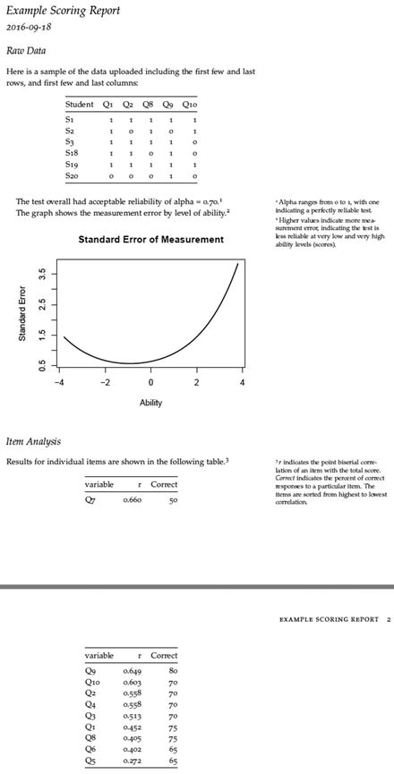
Figure 15-3. The PDF that downloads
Uploading to the Cloud
Our last task is to get our files from a local machine to the cloud instance. Remember, in prior chapters, we have not only used PuTTY to install Shiny Server on our cloud, but also used WinSCP to move files up to our cloud. We start WinSCP, reconnect, and ensure that on the left, local side we are in our Shiny application folder, while on our right, cloud server side we are in /home/ubuntu. We recall the result of that process in Figure 15-4.

Figure 15-4. WinSCP with PieChart_Time, slider_time, and Upload_hist Shiny applications all uploaded
From here, we access PuTTY and run the following code from the command line:
sudo cp -R ∼/Chapter15 /srv/shiny-server/ Remember, in an earlier chapter we adjusted our instance to allow access to certain ports from certain addresses. You may now verify that your application works by typing the following URL into any browser:
http://Your.Instance.IP.Address:3838/Chapter15/ Summary
In this, our last chapter, we built a dynamic document that can rapidly update based on new data. This update can even extend to graphics and inline ifelse statements, which allow the very narrative to morph based on new data. Additionally, we built a Shiny application that allows users with an Internet connection to upload a file to feed new data into such a report. Such reports can be download in many formats, although we chose PDF.
Throughout this text, we provided techniques for advanced data management, including connecting to various databases. Those techniques merge well with dynamic documents, and the ability to easily translate information in a data warehouse to actionable intelligence. Our final observation is that as data becomes more extensive, successful filtration and presentation of useful data become more vital skills in any field. Happy coding!