A breakthrough in machine learning would be worth ten Microsofts.
—Bill Gates1
While Katrina Lake liked to shop online, she knew the experience could be much better. The main problem: It was tough to find fashions that were personalized.
So began the inspiration for Stitch Fix, which Katrina launched in her Cambridge apartment while attending Harvard Business School in 2011 (by the way, the original name for the company was the less catchy “Rack Habit”). The site had a Q&A for its users—asking about size and fashion styles, just to name a few factors—and expert stylists would then put together curated boxes of clothing and accessories that were sent out monthly.
The concept caught on quickly, and the growth was robust. But it was tough to raise capital as many venture capitalists did not see the potential in the business. Yet Katrina persisted and was able to create a profitable operation—fairly quickly.
Along the way, Stitch Fix was collecting enormous amounts of valuable data, such as on body sizes and style preferences. Katrina realized that this would be ideal for machine learning. To leverage on this, she hired Eric Colson, who was the vice president of Data Science and Engineering at Netflix, his new title being chief algorithms officer.
This change in strategy was pivotal. The machine learning models got better and better with their predictions, as Stitch Fix collected more data—not only from the initial surveys but also from ongoing feedback. The data was also encoded in the SKUs.
The result: Stitch Fix saw ongoing improvement in customer loyalty and conversion rates. There were also improvements in inventory turnover, which helped to reduce costs.
But the new strategy did not mean firing the stylists. Rather, the machine learning greatly augmented their productivity and effectiveness.
The data also provided insights on what types of clothing to create. This led to the launch of Hybrid Designs in 2017, which is Stitch Fix’s private-label brand. This proved effective in dealing with the gaps in inventory.
By November 2017, Katrina took Stitch Fix public, raising $120 million. The valuation of the company was a cool $1.63 billion—making her one of the richest women in the United States.2 Oh, and at the time, she had a 14-month-old son!
Fast forward to today, Stitch Fix has 2.7 million customers in the United States and generates over $1.2 billion in revenues. There are also more than 100 data scientists on staff and a majority of them have PhDs in areas like neuroscience, mathematics, statistics, and AI.3
Our data science capabilities fuel our business. These capabilities consist of our rich and growing set of detailed client and merchandise data and our proprietary algorithms. We use data science throughout our business, including to style our clients, predict purchase behavior, forecast demand, optimize inventory and design new apparel.4
Historically, there’s been a gap between what you give to companies and how much the experience is improved. Big data is tracking you all over the web, and the most benefit you get from that right now is: If you clicked on a pair of shoes, you’ll see that pair of shoes again a week from now. We’ll see that gap begin to close. Expectations are very different around personalization, but importantly, an authentic version of it. Not, ‘You abandoned your cart and we’re recognizing that.’ It will be genuinely recognizing who you are as a unique human. The only way to do this scalably is through embracing data science and what you can do through innovation.5
OK then, what is machine learning really about? Why can it be so impactful? And what are some of the risks to consider?
In this chapter, we’ll answer these questions—and more.
What Is Machine Learning?
After stints at MIT and Bell Telephone Laboratories, Arthur L. Samuel joined IBM in 1949 at the Poughkeepsie Laboratory. His efforts helped boost the computing power of the company’s machines, such as with the development of the 701 (this was IBM’s first commercialized computer system).
But he also programmed applications. And there was one that would make history—that is, his computer checkers game. It was the first example of a machine learning system (Samuel published an influential paper on this in 19596). IBM CEO Thomas J. Watson, Sr., said that the innovation would add 15 points to the stock price!7
Then why was Samuel’s paper so consequential? By looking at checkers, he showed how machine learning works—in other words, a computer could learn and improve by processing data without having to be explicitly programmed. This was possible by leveraging advanced concepts of statistics, especially with probability analysis. Thus, a computer could be trained to make accurate predictions.
This was revolutionary as software development, at this time, was mostly about a list of commands that followed a workflow of logic.
To get a sense of how machine learning works, let’s use an example from the HBO TV comedy show Silicon Valley. Engineer Jian-Yang was supposed to create a Shazam for food. To train the app, he had to provide a massive dataset of food pictures. Unfortunately, because of time constraints, the app only learned how to identify…hot dogs. In other words, if you used the app, it would only respond with “hot dog” and “not hot dog.”
While humorous, the episode did a pretty good job of demonstrating machine learning. In essence, it is a process of taking in labeled data and finding relationships. If you train the system with hot dogs—such as thousands of images—it will get better and better at recognizing them.
Yes, even TV shows can teach valuable lessons about AI!
But of course, you still need much more. In the next section of the chapter, we’ll take a deeper look at the core statistics you need to know about machine learning. This includes the standard deviation, the normal distribution, Bayes’ theorem, correlation, and feature extraction.
Then we’ll cover topics like the use cases for machine learning, the general process, and the common algorithms.
Standard Deviation
The standard deviation measures the average distance from the mean. In fact, there is no need to learn how to calculate this (the process involves multiple steps) since Excel or other software can do this for you easily.
To understand the standard deviation, let’s take an example of the home values in your neighborhood. Suppose that the average is $145,000 and the standard deviation is $24,000. This means that one standard deviation below the average would be $133,000 ($145,000 – $12,000) and one standard deviation above the mean would come to $157,000 ($145,000 + $12,000). This gives us a way to quantify the variation in the data. That is, there is a spread of $24,000 from the average.
Next, let’s take a look at the data if, well, Mark Zuckerberg moves into your neighborhood and, as a result, the average jumps to $850,000 and the standard deviation is $175,000. But do these statistical metrics reflect the valuations? Not really. Zuckerberg’s purchase is an outlier. In this situation, the best approach may be instead to exclude his home.
The Normal Distribution
When plotted on a graph, the normal distribution looks like a bell (this is why another name for it is the “bell curve”). It represents the sum of probabilities for a variable. Interestingly enough, the normal curve is common in the natural world, as it reflects distributions of such things like height and weight.
A general approach when interpreting a normal distribution is to use the 68-95-99.7 rule. This estimates that 68% of the data items will fall within one standard deviation, 95% within two standard deviations, and 99.7% within three standard deviations.
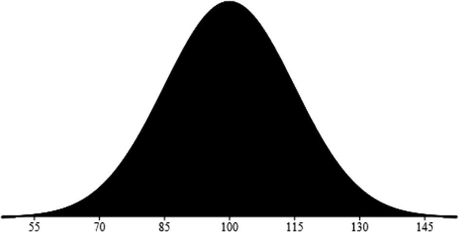
Normal distribution of IQ scores
Note that the peak in this graph is the average. So, if a person has an IQ of 145, then only 0.15% will have a higher score.
Now the curve may have different shapes, depending on the variation in the data. For example, if our IQ data has a large number of geniuses, then the distribution will skew to the right.
Bayes’ Theorem
As the name implies, descriptive statistics provides information about your data. We’ve already seen this with such things as averages and standard deviations.
But of course, you can go well beyond this—basically, by using the Bayes’ theorem. This approach is common in analyzing medical diseases, in which cause and effect are key—say for FDA (Federal Drug Administration) trials.
To understand how Bayes’ theorem works, let’s take an example. A researcher comes up with a test for a certain type of cancer, and it has proven to be accurate 80% of the time. This is known as a true positive.
But 9.6% of the time, the test will identify the person as having the cancer even though he or she does not have it, which is known as a false positive. Keep in mind that—in some drug tests—this percentage may be higher than the accuracy rate!
And finally, 1% of the population has the cancer.
Step #1: 80% accuracy rate × the chance of having the cancer (1%) = 0.008.
Step #2: The chance of not having the cancer (99%) × the 9.6% false positive = 0.09504.
Step #3: Then plug the above numbers into the following equation: 0.008 / (0.008 + 0.09504) = 7.8%.
Sounds kind of out of whack, right? Definitely. After all, how is it that a test, which is 90% accurate, has only a 7.8% probability of being right? But remember the accuracy rate is based on the measure of those who have the flu. And this is a small number since only 1% of the population has the flu. What’s more, the test is still giving off false positives. So Bayes’ theorem is a way to provide a better understanding of results—which is critical for systems like AI.
Correlation
A machine learning algorithm often involves some type of correlation among the data. A quantitative way to describe this is to use the Pearson correlation, which shows the strength of the relationship between two variables that range from 1 to –1 (this is the coefficient).
Greater than 0: This is where an increase in one variable leads to the increase in another. For example: Suppose that there is a 0.9 correlation between income and spending. If income increases by $1,000, then spending will be up by $900 ($1,000 X 0.9).
0: There is no correlation between the two variables.
Less than 0: Any increase in the variable means a decrease in another and vice versa. This describes an inverse relationship.
Then what is a strong correlation? As a general rule of thumb, it’s if the coefficient is +0.7 or so. And if it is under 0.3, then the correlation is tenuous.
All this harkens the old saying of “Correlation is not necessarily causation.” Yet when it comes to machine learning, this concept can easily be ignored and lead to misleading results.
The divorce rate in Maine has a 99.26% correlation with per capita consumption of margarine.
The age of Miss America has an 87.01% correlation with the murders by steam, hot vapors, and hot tropics.
The US crude oil imports from Norway have a 95.4% correlation with drivers killed in collision with a railway train.
There is a name for this: patternicity. This is the tendency to find patterns in meaningless noise.
Feature Extraction
In Chapter 2, we looked at selecting the variables for a model. The process is often called feature extraction or feature engineering.
An example of this would be a computer model that identifies a male or female from a photo. For humans, this is fairly easy and quick. It’s something that is intuitive. But if someone asked you to describe the differences, would you be able to? For most people, it would be a difficult task. However, if we want to build an effective machine learning model, we need to get feature extraction right—and this can be subjective.
Facial features
Features | Male |
|---|---|
Eyebrows | Thicker and straighter |
Face shape | Longer and larger, with more of a square shape |
Jawbone | Square, wider, and sharper |
Neck | Adam’s apple |
This just scratches the surface as I’m sure you have your own ideas or approaches. And this is normal. But this is also why such things as facial recognition are highly complex and subject to error.
Feature extraction also has some nuanced issues. One is the potential for bias. For example, do you have preconceptions of what a man or woman looks like? If so, this can result in models that give wrong results.
Because of all this, it’s a good idea to have a group of experts who can determine the right features. And if the feature engineering proves too complex, then machine learning is probably not a good option.
But there is another approach to consider: deep learning. This involves sophisticated models that find features in a data. Actually, this is one of the reasons that deep learning has been a major breakthrough in AI. We’ll learn more about this in the next chapter.
What Can You Do with Machine Learning?
As machine learning has been around for decades, there have been many uses for this powerful technology. It also helps that there are clear benefits, in terms of cost savings, revenue opportunities, and risk monitoring.
Predictive Maintenance: This monitors sensors to forecast when equipment may fail. This not only helps to reduce costs but also lessens downtime and boosts safety. In fact, companies like PrecisionHawk are actually using drones to collect data, which is much more efficient. The technology has proven quite effective for industries like energy, agriculture, and construction. Here’s what PrecisionHawk notes about its own drone-based predictive maintenance system: “One client tested the use of visual line of sight (VLOS) drones to inspect a cluster of 10 well pads in a three-mile radius. Our client determined that the use of drones reduced inspection costs by approximately 66%, from $80–$90 per well pad from traditional inspection methodology to $45–$60 per well pad using VLOS drone missions.”9
Recruiting Employees: This can be a tedious process since many resumes are often varied. This means it is easy to pass over great candidates. But machine learning can help in a big way. Take a look at CareerBuilder, which has collected and analyzed more than 2.3 million jobs, 680 million unique profiles, 310 million unique resumes, 10 million job titles, 1.3 billion skills, and 2.5 million background checks to build Hello to Hire. It’s a platform that has leveraged machine learning to reduce the number of job applications—for a successful hire—to an average of 75. The industry average, on the other hand, is about 150.10 The system also automates the creation of job descriptions, which even takes into account nuances based on the industry and location!
Customer Experience: Nowadays, customers want a personalized experience. They have become accustomed to this by using services like Amazon.com and Uber. With machine learning, a company can leverage its data to gain insight—learning about what really works. This is so important that it led Kroger to buy a company in the space, called 84.51°. It is definitely key that it has data on more than 60 million US households. Here’s a quick case study: For most of its stores, Kroger had bulk avocados, and only a few carried 4-packs. The conventional wisdom was that 4-packs had to be discounted because of the size disparity with the bulk items. But when applying machine learning analysis, this proved to be incorrect, as the 4-packs attracted new and different households like Millennials and ClickList shoppers. By expanding 4-packs across the chain, there was an overall increase in avocado sales.11
Finance: Machine learning can detect discrepancies, say with billing. But there is a new category of technology, called RPA (Robotic Process Automation), that can help with this (we’ll cover this topic in Chapter 5). It automates routine processes in order to help reduce errors. RPA also may use machine learning to detect abnormal or suspicious transactions.
Customer Service: The past few years has seen the growth in chatbots, which use machine learning to automate interactions with customers. We’ll cover this in Chapter 6.
Dating: Machine learning could help find your soul mate! Tinder, one of the largest dating apps, is using the technology to help improve the matches. For instance, it has a system that automatically labels more than 10 billion photos that are uploaded on a daily basis.
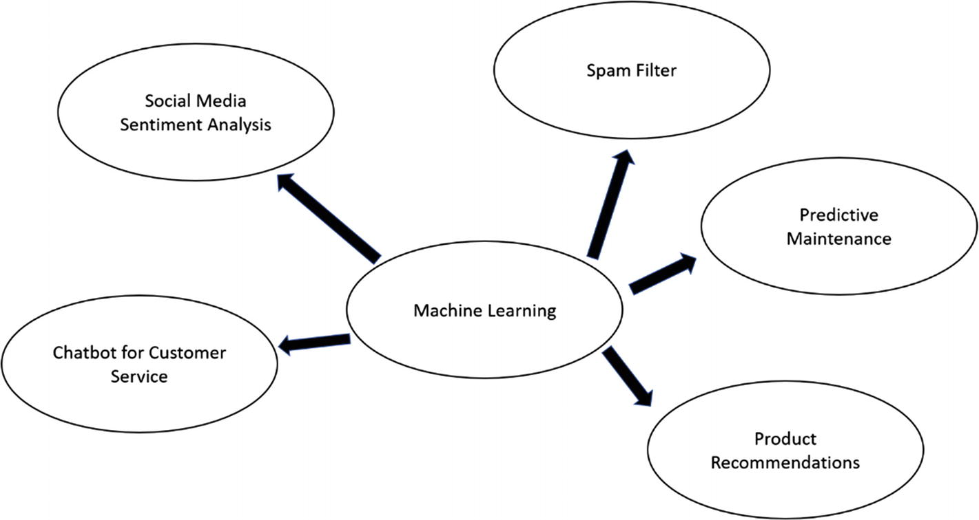
Applications for machine learning
The Machine Learning Process
To be successful with applying machine learning to a problem, it’s important to take a systematic approach. If not, the results could be way off base.
First of all, you need to go through a data process, which we covered in the prior chapter. When this is finished, it’s a good idea to do a visualization of the data. Is it mostly scattered? Or are there some patterns? If the answer is yes, then the data could be a good candidate for machine learning.
The goal of the machine learning process is to create a model, which is based on one or more algorithms. We develop this by training it. The goal is that the model should provide a high-degree of predictability.
Now let’s take a closer look at this (by the way, this will also be applicable for deep learning, which we’ll cover in the next chapter):
Step #1—Data Order
If your data is sorted, then this could skew the results. That is, the machine learning algorithm may detect this as a pattern! This is why it’s a good idea to randomize the order of the data.
Step #2—Choose a Model
You will need to select an algorithm. This will be an educated guess, which will involve a process of trial and error. In this chapter, we’ll look at the various algorithms available.
Step #3—Train the Model
The training data, which will be about 70% of the complete dataset, will be used to create the relationships in the algorithm. For example, suppose you are building a machine learning system to find the value of a used car. Some of the features will include the year manufactured, make, model, mileage, and condition. By processing this training data, the algorithm will calculate the weights for each of these factors.
Example: Suppose we are using a linear regression algorithm, which has the following format:
y = m * x + b
In the training phase, the system will come up with the values for m (which is the slope on a graph) and b (which is the y-intercept).
Step #4—Evaluate the Model
You will put together test data, which is the remaining 30% of the dataset. It should be representative of the ranges and type of information in the training data.
With the test data, you can see if the algorithm is accurate. In our used car example, are the market values consistent with what’s happening in the real world?
Note
With the training and test data, there must not be any intermingling. This can easily lead to distorted results. Interestingly enough, this is a common mistake.
Now accuracy is one measure of the success of the algorithm. But this can, in some cases, be misleading. Consider the situation with fraud deduction. There are usually a small number of features when compared to a dataset. But missing one could be devastating, costing a company millions of dollars in losses.
This is why you might want to use other approaches like Bayes’ theorem.
Step #5—Fine-Tune the Model
In this step, we can adjust the values of the parameters in the algorithm. This is to see if we can get better results.
When fine-tuning the model, there may also be hyperparameters. These are parameters that cannot be learned directly from the training process.
Applying Algorithms
Some algorithms are quite easy to calculate, while others require complex steps and mathematics. The good news is that you usually do not have to compute an algorithm because there are a variety of languages like Python and R that make the process straightforward.
As for machine learning, an algorithm is typically different from a traditional one. The reason is that the first step is to process data—and then, the computer will start to learn.
Even though there are hundreds of machine learning algorithms available, they can actually be divided into four major categories: supervised learning, unsupervised learning, reinforcement learning, and semi-supervised learning. We’ll take a look at each.
Supervised Learning
Supervised learning uses labeled data. For example, suppose we have a set of photos of thousands of dogs. The data is considered to be labeled if each photo identifies each for the breed. For the most part, this makes it easier to analyze since we can compare our results with the correct answer.
One of the keys with supervised learning is that there should be large amounts of data. This helps to refine the model and produce more accurate results.
But there is a big issue: The reality is that much of the data available is not labeled. In addition, it could be time consuming to provide labels if there is a massive dataset.
Yet there are creative ways to deal with this, such as with crowdfunding. This is how the ImageNet system was built, which was a breakthrough in AI innovation. But it still took several years to create it.
Or, in some cases, there can be automated approaches to label data. Take the example of Facebook. In 2018, the company announced—at its F8 developers conference—it leveraged its enormous database of photos from Instagram, which were labeled with hashtags.12
Granted, this approach had its flaws. A hashtag may give a nonvisual description of the photo—say #tbt (which is “throwback Thursday)—or could be too vague, like #party. This is why Facebook called its approach “weakly supervised data.” But the talented engineers at the company found some ways to improve the quality, such as by building a sophisticated hashtag prediction model.
All in all, things worked out quite well. Facebook’s machine learning model , which included 3.5 billion photos, had an accuracy rate of 85.4%, which was based on the ImageNet recognition benchmark. It was actually the highest recorded in history, by 2%.
Since a single machine would have taken more than a year to complete the model training, we created a way to distribute the task across up to 336 GPUs, shortening the total training time to just a few weeks. With ever-larger model sizes—the biggest in this research is a ResNeXt 101-32x48d with over 861 million parameters—such distributed training is increasingly essential. In addition, we designed a method for removing duplicates to ensure we don’t accidentally train our models on images that we want to evaluate them on, a problem that plagues similar research in this area.13
Improved ranking in the newsfeed
Better detection of objectionable content
Auto generation of captions for the visually impaired
Unsupervised Learning
Unsupervised learning is when you are working with unlabeled data. This means that you will use deep learning algorithms to detect patterns.
Euclidean Metric: This is a straight line between two data points. The Euclidean metric is quite common with machine learning.
Cosine Similarity Metric: As the name implies, you will use a cosine to measure the angle. The idea is to find similarities between two data points in terms of the orientation.
Manhattan Metric: This involves taking the sum of the absolute distances of two points on the coordinates of a graph. It’s called the “Manhattan” because it references the city’s street layout, which allows for shorter distances for travel.
In terms of use cases for clustering, one of the most common is customer segmentation, which is to help better target marketing messages. For the most part, a group that has similar characteristics is likely to share interests and preferences.
Another application is sentiment analysis, which is where you mine social media data and find the trends. For a fashion company, this can be crucial in understanding how to adapt the styles of the upcoming line of clothes.
Association: The basic concept is that if X happens, then Y is likely to happen. Thus, if you buy my book on AI, you will probably want to buy other titles in the genre. With association, a deep learning algorithm can decipher these kinds of relationships. This can result in powerful recommendation engines.
Anomaly Detection: This identifies outliers or anomalous patterns in the dataset, which can be helpful with cybersecurity applications. According to Asaf Cidon, who is the VP of Email Security at Barracuda Networks: “We’ve found that by combining many different signals—such as the email body, header, the social graph of communications, IP logins, inbox forwarding rules, etc.—we’re able to achieve an extremely high precision in detecting social engineering attacks, even though the attacks are highly personalized and crafted to target a particular person within a particular organization. Machine learning enables us to detect attacks that originate from within the organization, whose source is a legitimate mailbox of an employee, which would be impossible to do with a static one-size-fits-all rule engine.”14
Autoencoders: With this, the data will be put into a compressed form, and then it will be reconstructed. From this, new patterns may emerge. However, the use of autoencoders is rare. But it could be shown to be useful in helping with applications like reducing noise in data.
Consider that many AI researchers believe that unsupervised learning will likely be critical for the next level of achievements. According to a paper in Nature by Yann LeCun, Geoffrey Hinton, and Yoshua Bengio, “We expect unsupervised learning to become far more important in the longer term. Human and animal learning is largely unsupervised: we discover the structure of the world by observing it, not by being told the name of every object.”15
Reinforcement Learning
When you were a kid and wanted to play a new sport, chances were you did not read a manual. Instead, you observed what other people were doing and tried to figure things out. In some situations, you made mistakes and lost the ball as your teammates would show their displeasure. But in other cases, you made the right moves and scored. Through this trial-and-error process, your learning was improved based on positive and negative reinforcement.
Games: They are ideal for reinforcement learning since there are clear-cut rules, scores, and various constraints (like a game board). When building a model, you can test it with millions of simulations, which means that the system will quickly get smarter and smarter. This is how a program can learn to beat the world champion of Go or chess.
Robotics: A key is being able to navigate within a space—and this requires evaluating the environment at many different points. If the robot wants to move to, say, the kitchen, it will need to navigate around furniture and other obstacles. If it runs into things, there will be a negative reinforcement action.
Semi-supervised Learning
This is a mix of supervised and unsupervised learning. This arises when you have a small amount of unlabeled data. But you can use deep learning systems to translate the unsupervised data to supervised data—a process that is called pseudo-labeling. After this, you can then apply the algorithms.
An interesting use case of semi-supervised learning is the interpretation of MRIs. A radiologist can first label the scans, and after this, a deep learning system can find the rest of the patterns.
Common Types of Machine Learning Algorithms
There is simply not enough room in this book to cover all the machine learning algorithms! Instead, it’s better to focus on the most common ones.
Supervised Learning : You can boil down the algorithms to two variations. One is classification, which divides the dataset into common labels. Examples of the algorithms include Naive Bayes Classifier and k-Nearest Neighbor (neural networks will be covered in Chapter 4). Next, there is regression, which finds continuous patterns in the data. For this, we’ll take a look at linear regression, ensemble modelling, and decision trees.
Unsupervised Learning : In this category, we’ll look at clustering. For this, we’ll cover k-Means clustering .
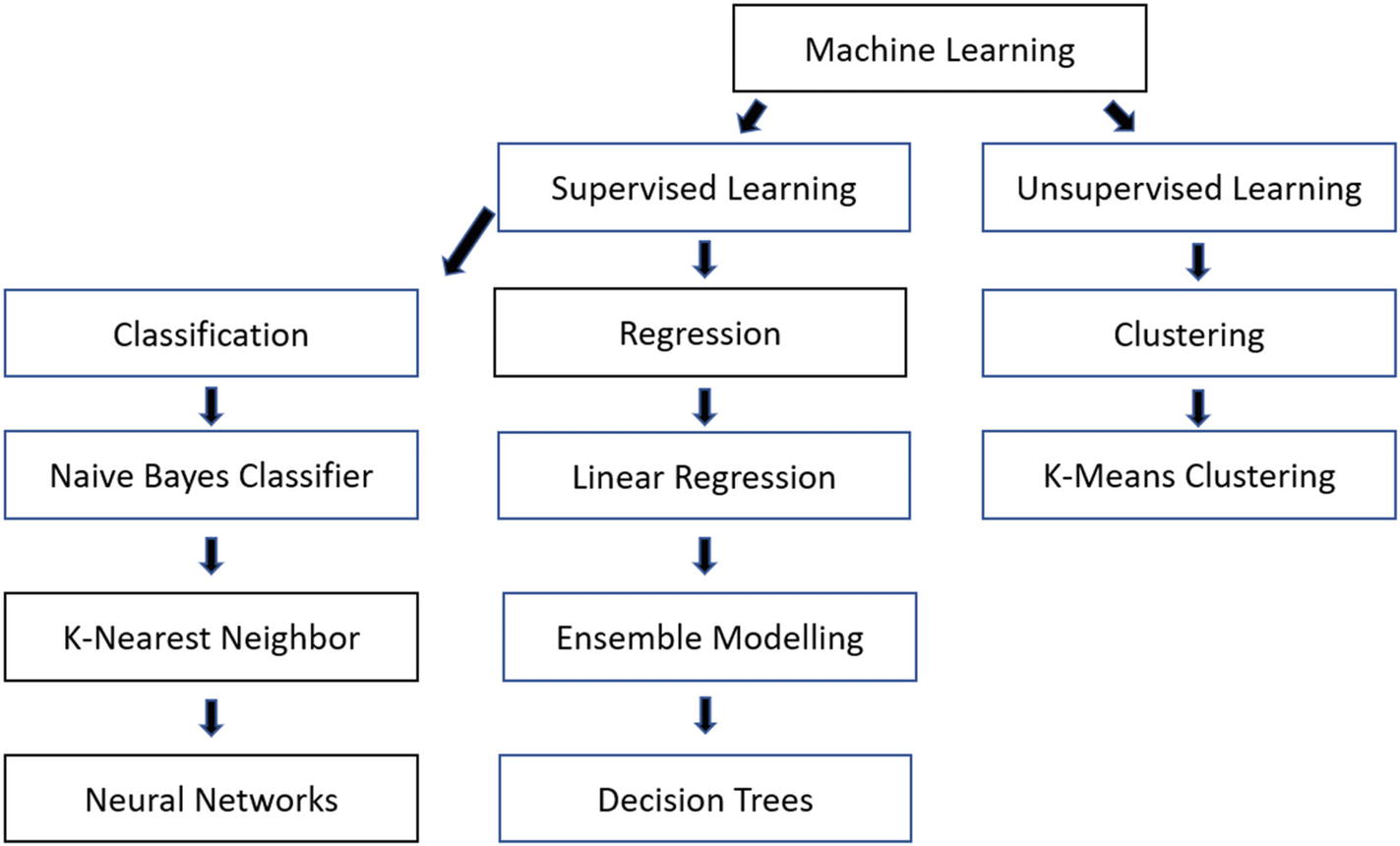
General framework for machine learning algorithms
Naïve Bayes Classifier (Supervised Learning/Classification)
Earlier in this chapter, we looked at Bayes’ theorem. As for machine learning, this has been modified into something called the Naïve Bayes Classifier. It is “naïve” because the assumption is that the variables are independent from each other—that is, the occurrence of one variable has nothing to do with the others. True, this may seem like a drawback. But the fact is that the Naïve Bayes Classifier has proven to be quite effective and fast to develop.
There is another assumption to note as well: the a priori assumption. This says that the predictions will be wrong if the data has changed.
Bernoulli: This is if you have binary data (true/false, yes/no).
Multinomial: This is if the data is discrete, such as the number of pages of a book.
Gaussian: This is if you are working with data that conforms to a normal distribution.
A common use case for Naïve Bayes Classifiers is text analysis. Examples include email spam detection, customer segmentation, sentiment analysis , medical diagnosis, and weather predictions. The reason is that this approach is useful in classifying data based on key features and patterns.
To see how this is done, let’s take an example: Suppose you run an e-commerce site and have a large database of customer transactions. You want to see how variables like product review ratings, discounts, and time of year impact sales.
Customer transactions dataset
Discount | Product Review | Purchase |
|---|---|---|
Yes | High | Yes |
Yes | Low | Yes |
No | Low | No |
No | Low | No |
No | Low | No |
No | High | Yes |
Yes | High | No |
Yes | Low | Yes |
No | High | Yes |
Yes | High | Yes |
No | High | No |
No | Low | Yes |
Yes | High | Yes |
Yes | Low | No |
Discount frequency table
Purchase | |||
|---|---|---|---|
Yes | No | ||
Discount | Yes | 19 | 1 |
Yes | 5 | 5 | |
Product review frequency table
Purchase | ||||
|---|---|---|---|---|
Yes | No | Total | ||
Product Review | High | 21 | 2 | 11 |
Low | 3 | 4 | 8 | |
Total | 24 | 6 | 19 | |
Product review probability table
Purchase | ||||
|---|---|---|---|---|
Yes | No | |||
Product Reviews | High | 9/24 | 2/6 | 11/30 |
Low | 7/24 | 1/6 | 8/30 | |
24/30 | 6/30 | |||
Using this chart, we can see that the probability of a purchase when there is a low product review is 7/24 or 29%. In other words, the Naïve Bayes Classifier allows more granular predictions within a dataset. It is also relatively easy to train and can work well with small datasets.
K-Nearest Neighbor (Supervised Learning/Classification)
The k-Nearest Neighbor (k-NN ) is a method for classifying a dataset (k represents the number of neighbors). The theory is that those values that are close together are likely to be good predictors for a model. Think of it as “Birds of a feather flock together.”
A use case for k-NN is the credit score, which is based on a variety of factors like income, payment histories, location, home ownership, and so on. The algorithm will divide the dataset into different segments of customers. Then, when there is a new customer added to the base, you will see what cluster he or she falls into—and this will be the credit score.
K-NN is actually simple to calculate. In fact, it is called lazy learning because there is no training process with the data.
To use k-NN, you need to come up with the distance between the nearest values. If the values are numerical, it could be based on a Euclidian distance, which involves complicated math. Or, if there is categorical data, then you can use an overlap metric (this is where the data is the same or very similar).
Next, you’ll need to identify the number of neighbors. While having more will smooth the model, it can also mean a need for huge amount of computational resources. To manage this, you can assign higher weights to data that are closer to their neighbors.
Linear Regression (Supervised Learning/Regression)
Linear regression shows the relationship between certain variables. The equation—assuming there is enough quality data—can help predict outcomes based on inputs.
Chart for hours of study and grades
Hours of Study | Grade Percentage |
|---|---|
1 | 0.75 |
1 | 0.69 |
1 | 0.71 |
3 | 0.82 |
3 | 0.83 |
4 | 0.86 |
5 | 0.85 |
5 | 0.89 |
5 | 0.84 |
6 | 0.91 |
6 | 0.92 |
7 | 0.95 |
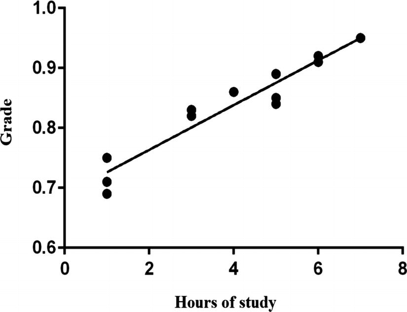
This is a plot of a linear regression model that is based on hours of study
From this, we get the following equation:
Grade = Number of hours of study × 0.03731 + 0.6889
Then, let’s suppose you study 4 hours for the exam . What will be your estimated grade? The equation tells us how:
0.838 = 4 × 0.03731 + 0.6889
How accurate is this? To help answer this question, we can use a calculation called R-squared. In our case, it is 0.9180 (this ranges from 0 to 1). The closer the value is to 1, the better the fit. So 0.9180 is quite high. It means that the hours of study explains 91.8% of the grade on the exam.
Now it’s true that this model is simplistic. To better reflect reality, you can add more variables to explain the grade on the exam—say the student’s attendance. When doing this, you will use something called multivariate regression .
Note
If the coefficient for a variable is quite small, then it might be a good idea to not include it in the model.
Sometimes data may not be in a straight line either, in which case the regression algorithm will not work . But you can use a more complex version, called polynomial regression.
Decision Tree (Supervised Learning/Regression)
No doubt, clustering may not work on some datasets. But the good news is that there are alternatives, such as a decision tree. This approach generally works better with nonnumerical data.
The start of a decision tree is the root node, which is at the top of the flow chart. From this point, there will be a tree of decision paths, which are called splits. At these points, you will use an algorithm to make a decision, and there will be a probability computed. At the end of the tree will be the leaf (or the outcome).
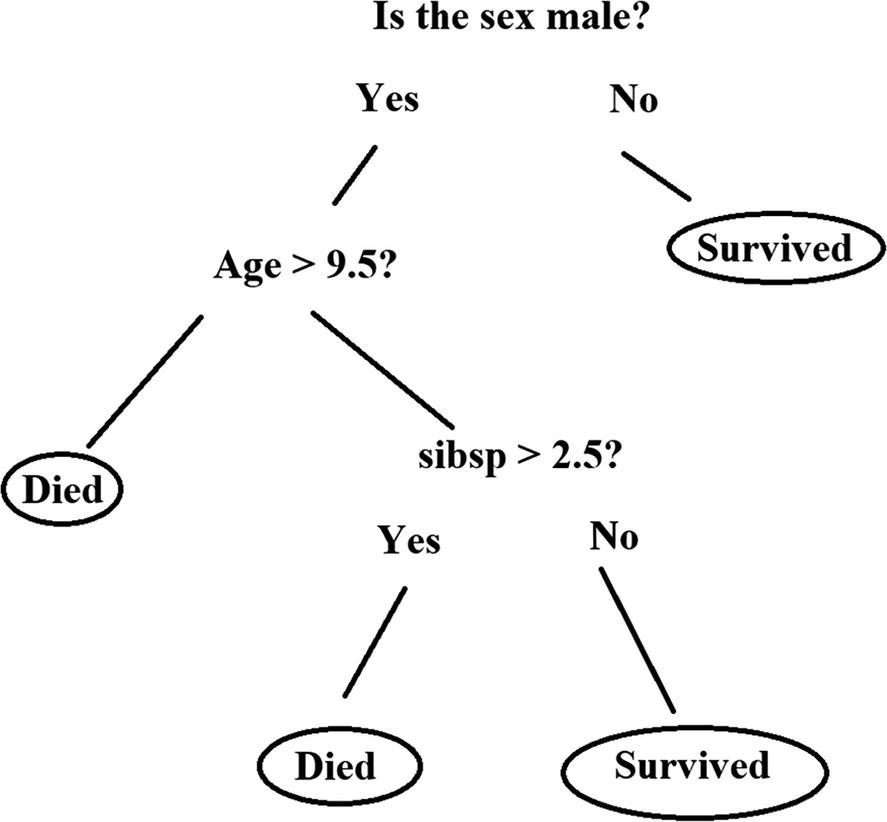
This is a basic decision tree algorithm for predicting the survival of the Titanic
There are clear advantages for decision trees. They are easy to understand, work well with large datasets, and provide transparency with the model.
However, decision trees also have drawbacks. One is error propagation. If one of the splits turns out to be wrong, then this error can cascade throughout the rest of the model!
Next, as the decision trees grow, there will be more complexity as there will be a large number of algorithms. This could ultimately result in lower performance for the model .
Ensemble Modelling (Supervised Learning/Regression)
Ensemble modelling means using more than one model for your predictions. Even though this increases the complexity, this approach has been shown to generate strong results.
To see this in action, take a look at the “Netflix Prize,” which began in 2006. The company announced it would pay $1 million to anyone or any team that could improve the accuracy of its movie recommendation system by 10% or more. Netflix also provided a dataset of over 100 million ratings of 17,770 movies from 480,189 users.16 There would ultimately be more than 30,000 downloads.
Why did Netflix do all this? A big reason is that the company’s own engineers were having trouble making progress. Then why not give it to the crowd to figure out? It turned out to be quite ingenious—and the $1 million payout was really modest compared to the potential benefits.
The contest certainly stirred up a lot of activity from coders and data scientists, ranging from students to employees at companies like AT&T.
Netflix also made the contest simple. The main requirement was that the teams had to disclose their methods , which helped boost the results (there was even a dashboard with rankings of the teams).
But it was not until 2009 that a team—BellKor’s Pragmatic Chaos—won the prize. Then again, there were considerable challenges.
So how did the winning team pull it off? The first step was to create a baseline model that smoothed out the tricky issues with the data. For example, some movies only had a handful of ratings, whereas others had thousands. Then there was the thorny problem where there were users who would always rate a movie with one star. To deal with these matters, BellKor used machine learning to predict ratings in order to fill the gaps.
A system may wind up recommending the same films to many users.
Some movies may not fit well within genres. For example, Alien is really a cross of science fiction and horror.
There were movies, like Napoleon Dynamite, that proved extremely difficult for algorithms to understand.
Ratings of a movie would often change over time.
The winning team used ensemble modelling, which involved hundreds of algorithms. They also used something called boosting, which is where you build consecutive models. With this, the weights in the algorithms are adjusted based on the results of the previous model, which help the predictions get better over time (another approach, called bagging, is when you build different models in parallel and then select the best one).
But in the end, BellKor found the solutions. However, despite this, Netflix did not use the model! Now it’s not clear why this was the case. Perhaps it was that Netflix was moving away from five-star ratings anyway and was more focused on streaming. The contest also had blowback from people who thought there may have been privacy violations.
Regardless, the contest did highlight the power of machine learning—and the importance of collaboration.
K-Means Clustering (Unsupervised/Clustering)
The k-Means clustering algorithm, which is effective for large datasets, puts similar, unlabeled data into different groups. The first step is to select k, which is the number of clusters. To help with this, you can perform visualizations of that data to see if there are noticeable grouping areas.
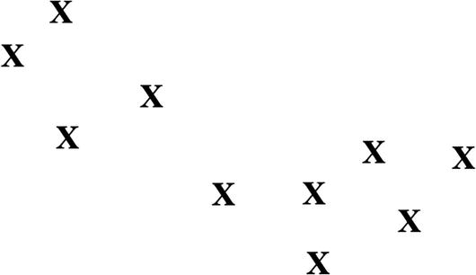
The initial plot for a dataset
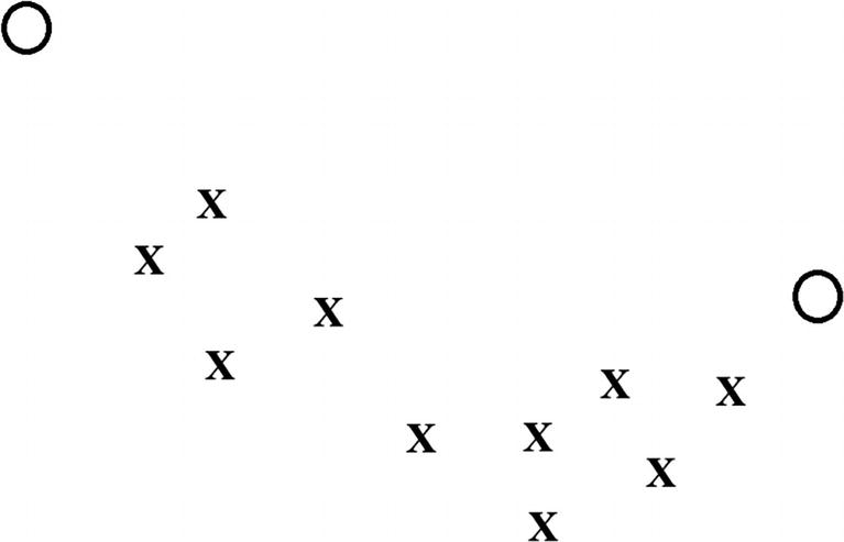
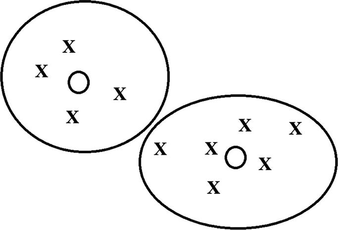
This chart shows two centroids—represented by circles—that are randomly placed
Through iterations, the k-Means algorithm gets better at grouping the data
Granted, this is a simple illustration. But of course, with a complex dataset, it will be difficult to come up with the number of initial clusters. In this situation, you can experiment with different k values and then measure the average distances. By doing this multiple times, there should be more accuracy.
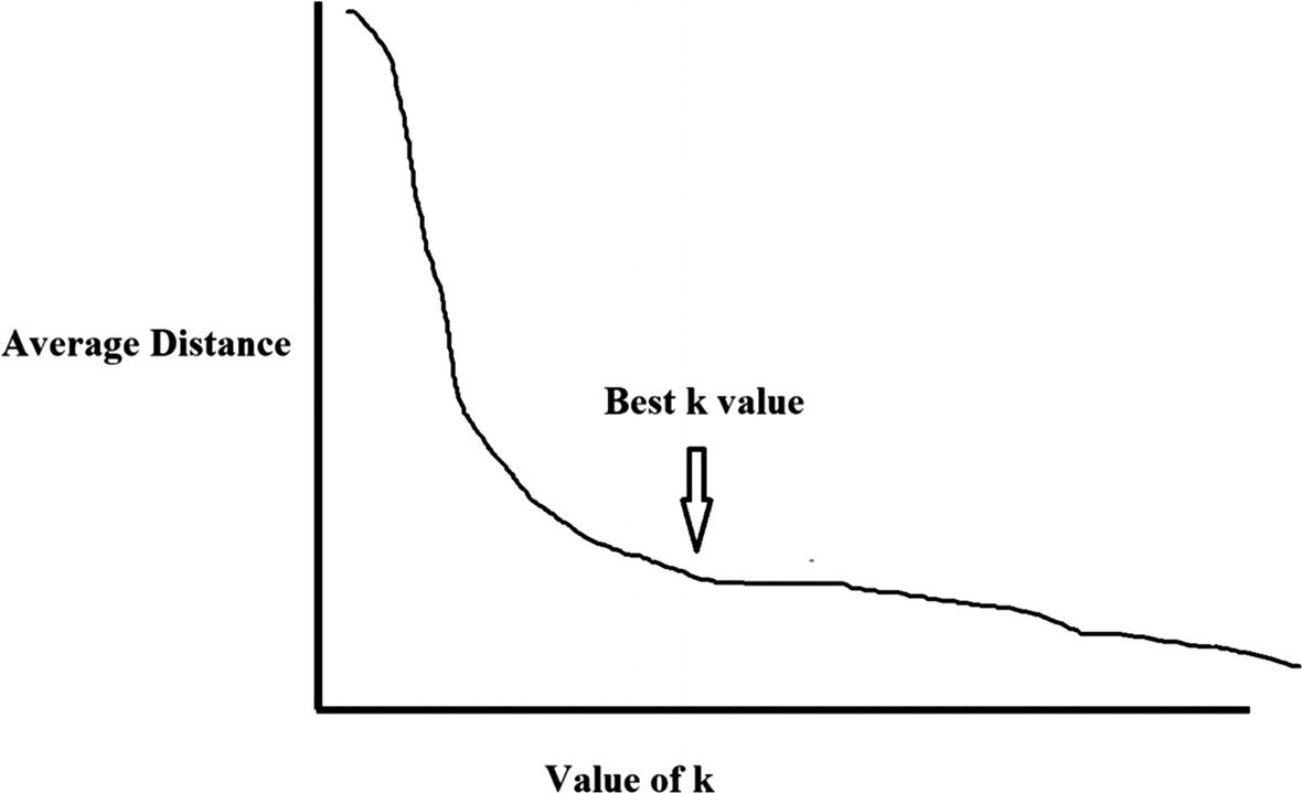
This shows the optimal point of the k value in the k-Means algorithm
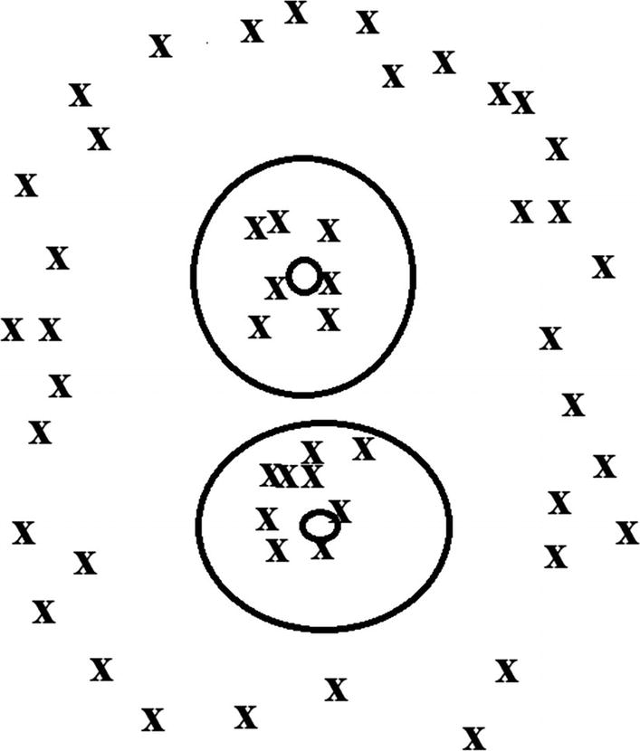
Here’s a demonstration where k-Means does not work with nonspherical data
With this, the k-Means algorithm would likely not pick up on the surrounding data, even though it has a pattern. But there are some algorithms that can help, such as DBScan (density-based spatial clustering of applications with noise), which is meant to handle a mix of widely varying sizes of datasets. Although, DBScan can require lots of computational power.
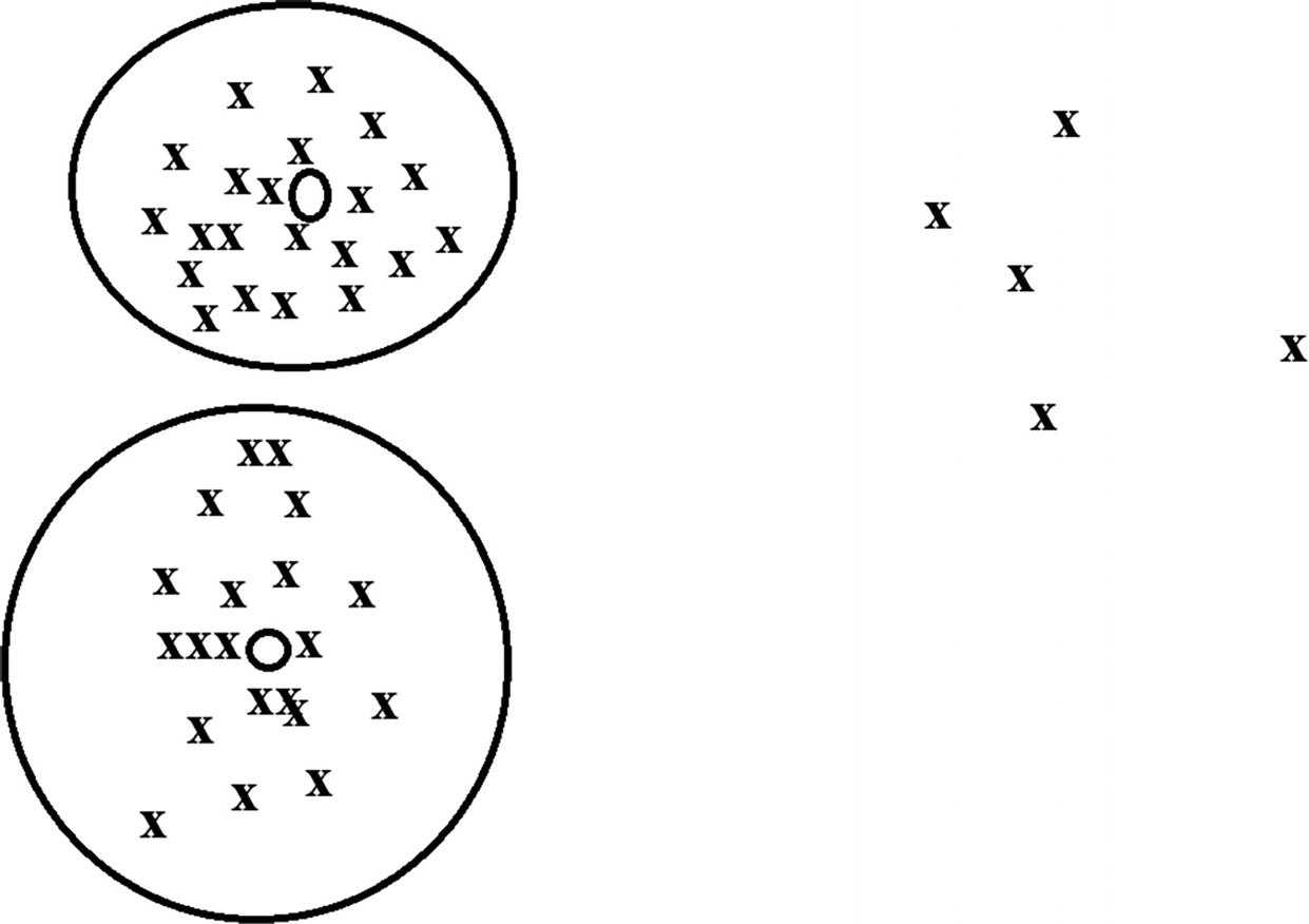
If there are areas of thin data, the k-Means algorithm may not pick them up
Conclusion
These algorithms can get complicated and do require strong technical skills. But it is important to not get too bogged down in the technology. After all, the focus is to find ways to use machine learning to accomplish clear objectives.
Again, Stich Fix is a good place to get guidance on this. In the November issue of the Harvard Business Review, the company’s chief algorithms officer, Eric Colson, published an article, “Curiosity-Driven Data Science.”17 In it, he provided his experiences in creating a data-driven organization.
At the heart of this is allowing data scientists to explore new ideas, concepts, and approaches. This has resulted in AI being implemented across core functions of the business like inventory management, relationship management, logistics, and merchandise buying. It has been transformative, making the organization more agile and streamlined. Colson also believes it has provided “a protective barrier against competition.”
Data Scientists: They should not be part of another department. Rather, they should have their own, which reports directly to the CEO. This helps with focusing on key priorities as well as having a holistic view of the needs of the organization.
Experiments: When a data scientist has a new idea, it should be tested on a small sample of customers. If there is traction, then it can be rolled out to the rest of the base.
Resources: Data scientists need full access to data and tools. There should also be ongoing training.
Generalists: Hire data scientists who span different domains like modelling, machine learning, and analytics (Colson refers to these people as “full-stack data scientists”). This leads to small teams—which are often more efficient and productive.
Culture: Colson looks for values like “learning by doing, being comfortable with ambiguity, balancing long-and short-term returns.”
Key Takeaways
Machine learning, whose roots go back to the 1950s, is where a computer can learn without being explicitly programmed. Rather, it will ingest and process data by using sophisticated statistical techniques.
An outlier is data that is far outside the rest of the numbers in the dataset.
The standard deviation measures the average distance from the mean.
The normal distribution—which has a shape like a bell—represents the sum of probabilities for a variable.
The Bayes’ theorem is a sophisticated statistical technique that provides a deeper look at probabilities.
A true positive is when a model makes a correct prediction. A false positive, on the other hand, is when a model prediction shows that the result is true even though it is not.
The Pearson correlation shows the strength of the relationship between two variables that range from 1 to -1.
Feature extraction or feature engineering describes the process of selecting variables for a model. This is critical since even one wrong variable can have a major impact on the results.
Training data is what is used to create the relationships in an algorithm. The test data, on the other hand, is used to evaluate the model.
Supervised learning uses labeled data to create a model, whereas unsupervised learning does not. There is also semi-supervised learning, which uses a mix of both approaches.
Reinforcement learning is a way to train a model by rewarding accurate predictions and punishing those that are not.
The k-Nearest Neighbor (k-NN ) is an algorithm based on the notion that values that are close together are good predictors for a model.
Linear regression estimates the relationship between certain variables. The R-squared will indicate the strength of the relationship.
A decision tree is a model that is based on a workflow of yes/no decisions.
An ensemble model uses more than one model for the predictions.
The k-Means clustering algorithm puts similar unlabeled data into different groups.