
Data processing layer
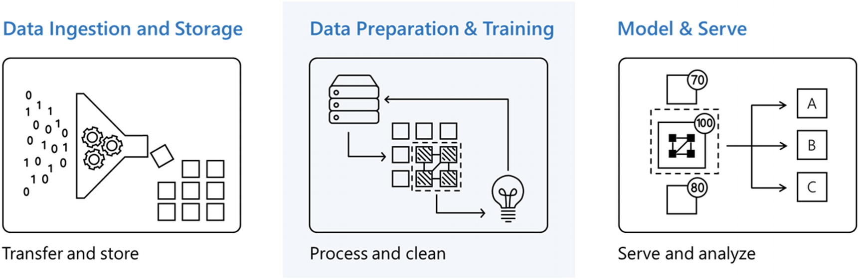
Data Preparation and Training
Real-time and batch mode data processing
- 1.
Data cleaning: Process to detect and remove noisy, inaccurate, and unwanted data
- 2.
Data transformation: Normalize data to avoid too many joins and improve consistency and completeness of data
- 3.
Data reduction: Data reduction is aggregation of data and identifying data samples needed to train the ML models.
- 4.
Data discretization: Process to convert data into right-sized partitions or internals to bring uniformity
- 5.
Text cleaning: Process to identify the data based on the target use case, and further cleaning the data that is not needed
- 1.
Data engineers: Data engineers manage the entire pipeline of ingestion and storage of data. The focus area for data engineers is to design, build, and arrange data pipelines. They are equipped with skills like advanced programming and analytics, distributed systems, and data pipelines.
- 2.
Data scientists: ML developers and data scientists focus on exploratory data analysis and building ML models. They are responsible for creating hypothesis testing, analyzing and building ML models using clean data. They are equipped with skills like ML/AI knowledge, advanced statistics, and advanced analytics.
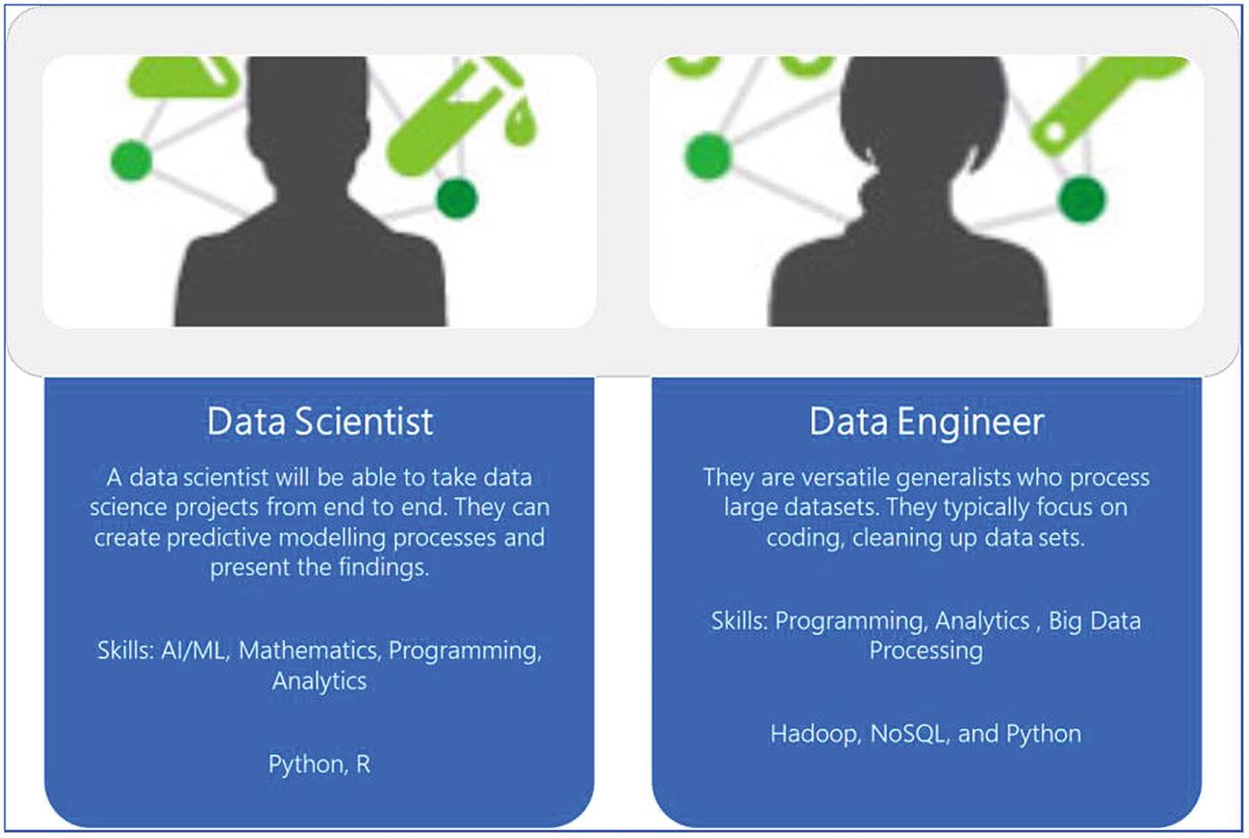
Roles of data scientist and data engineer
Let’s further discuss the data preparation and training phase.
Data Preparation
- 1.
Process real-time data streams
- 2.
Process batch mode data
Process Real-Time Data Streams
- 1.Managed service - PaaS (platform as a Service)
- a.
Apache Kafka on HDInsight Cluster
- b.
Event Hub
- c.
IoT Hub
- a.
- 2.Infrastructure as a service
- d.
Apache Kafka
- e.
Rabbit MQ
- f.
Zero MQ
- g.
Marketplace solutions
- d.
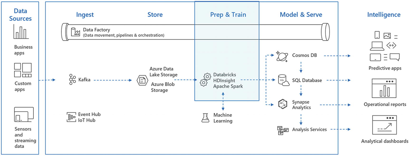
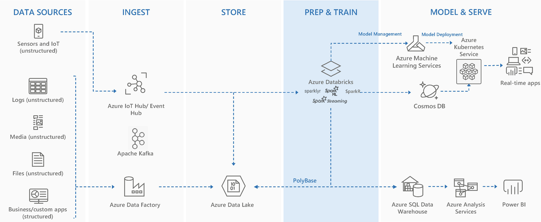
In Chapter 4, real-time streams and batch data ingestion were discussed in detail. Moreover, there were exercises based on Apache Kafka, Event hubs, and IoT hubs. In the coming sections, let’s delve deeper into the prep and train phase and discuss how the data coming from the aforementioned data sources can be processed.
- 1.
Apache Spark on HDInsight clusters or Databricks
- 2.
Stream analytics
Apache Spark
Microsoft Azure has managed Apache Spark on HDInsight cluster and Azure Databricks cluster, which can be spun with a few clicks. Apache Spark can be used for both streaming and batch mode data processing.
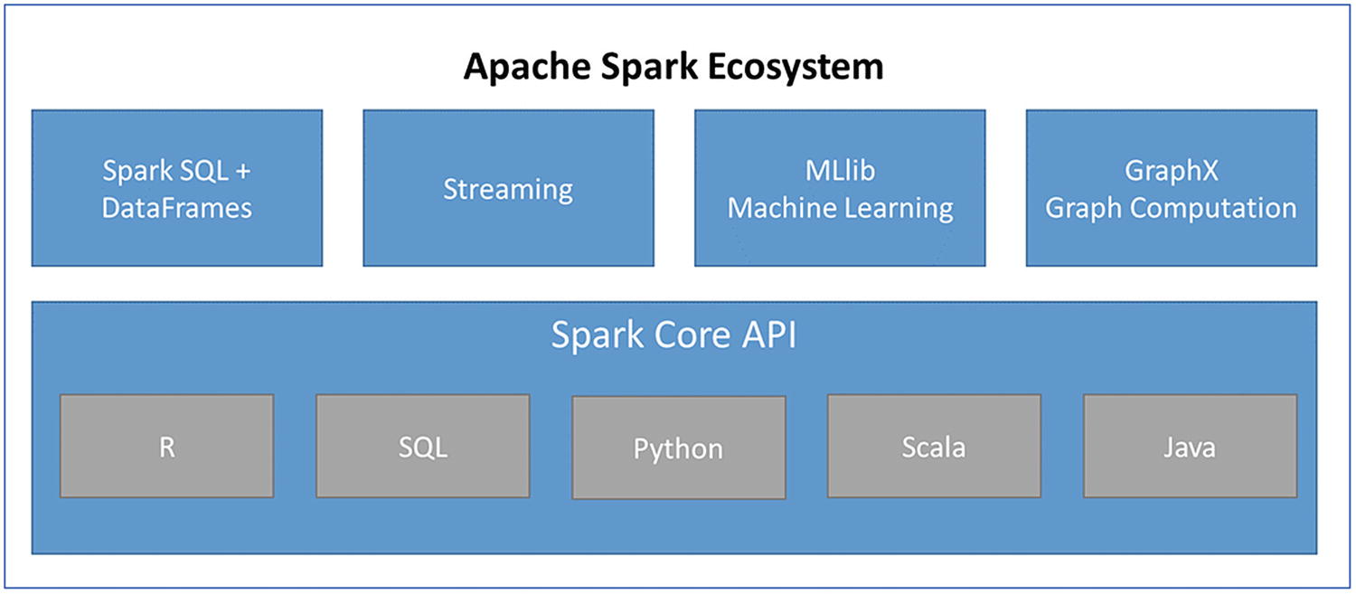
Apache Spark ecosystem
Spark DataFrames: A DataFrame is a distributed collection of data organized into named columns. It is conceptually equivalent to a table in a relational database or a data frame in R/Python. DataFrames can be built from structured data sources, tables in Hive, RDDs, or databases. DataFrames can be constructed in R, Python, Scala, and Java languages.
Spark SQL: For structured data processing, Spark provides Spark SQL, which can be used to execute SQL queries on structured data. Spark SQL provides Spark with more information about the type and structure of the data, which helps Spark to provide query processing optimization as compared with DataFrames.
Spark Streaming: For streaming data processing, Spark provides Spark Streaming. It enables distributed, scalable, fault-tolerant, high-throughput processing of real-time streaming data. Data in this case can be ingested through sources like Kafka, Kinesis, Flume, or TCP sockets. It supports functions like map, reduce, and join window, which can be used for high level processing. Further, processed data can be pushed to databases, filesystems, or BI tools.
Spark MLlib libraries: These are Spark’s machine learning libraries, which make machine learning distributed, scalable, and efficient. They provide common algorithms like classification, regression, clustering, and collaborative filtering. Moreover, Spark MLlib has the capability to build complete data science models. Capabilities like features extraction, transformation, and selection of data or even tools for constructing, evaluating, and tuning ML based pipelines are available with Spark MLlib.
GraphX : This component in Spark helps in processing graphs through parallel computation; its use cases include data exploration and cognitive analytics.
Spark Core API: It provides support for languages like Scala, Java, SQL, R, and Python.
- 1.
Programming APIs
- 2.
Catalyst optimizer
- 3.
Structured streaming
Programming APIs
Resilient Distributed Dataset
DataFrame
Dataset
Resilient Distributed Dataset (RDD): In the earlier version of Spark, RDD was the primary API. RDD is an immutable distributed data collection, which can be partitioned over the Spark cluster to make data processing run in parallel. Activities like transformation and actions can be performed over RDDs. RDDs are preferably used when low-level access or control is required over the datasets or when the data is unstructured, like media files or free text data, and there is no need to impose any schema. Moreover, data manipulation is to be achieved through pure functional programming.
DataFrame: Just like RDDs, they are also immutable distributed data collections, but here data is organized into columns just like tables in relational databases. It gives options to the developers to provide a structure to the data, thus it has a high-level abstraction. DataFrames are much simpler to understand and work with, as this API provides many functions to manipulate the data as well.
Dataset: Dataset is an extension to DataFrame. It has two API characteristics, which are strongly typed and untyped. By default, they are strongly typed JVM objects. Datasets provide better performance and optimization over DataFrames, as they expose expressions and data fields to a query planner through a catalyst query optimizer and Tungsten execution engine. Since Spark 2.0, DataFrame APIs have been merged with Dataset APIs to provide a unified data processing capability across the multiple Spark libraries.
- 1.
high-level abstraction and simplified APIs are needed.
- 2.
filters, map, aggregation, sum, or lambda functions on structured or semistructured data is needed.
- 3.
type safety at compile time and high level of optimization is needed.
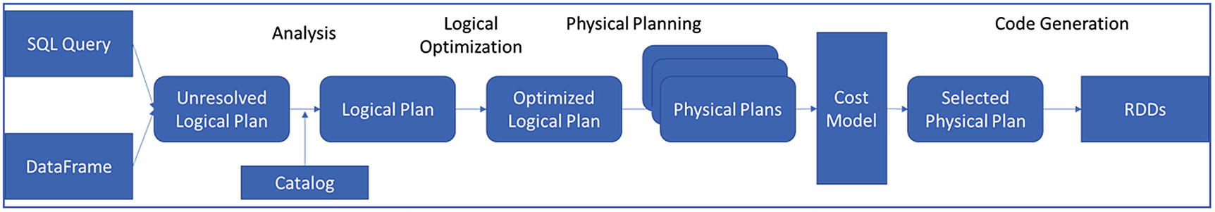
Catalyst optimizer
DataFrames and Datasets are based on the Spark SQL engine. Spark SQL consists of a catalyst optimizer, which can be used by both DataFrame and Dataset APIs. The Catalyst optimizer (Figure 6-5) is an extensible query optimizer; it leverages advanced programming languages features like Scala’s pattern matching and quasiquotes.
Pattern matching is a mechanism to check a value against a pattern; a pattern match includes a sequence of alternatives, each starting with the keyword case. Each alternative includes a pattern and one or more expressions, which will be evaluated if the pattern matches. An arrow symbol => separates the pattern from the expressions.
Catalyst optimizer
Structured streaming
Apache 1.X version had a concept called micro batching: based on a specific interval, the streaming data will be gathered and processed. It used to create an RDD based on the intervals mentioned for micro batch. Moreover, APIs for streaming data and batch data were not fully compatible.
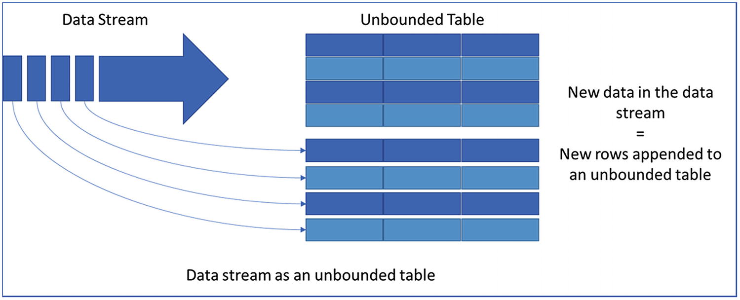
Unbounded table to support structured streaming
Continuous Application
Updating backend data in real time
Extract, transform, load (ETL)
Machine learning on continuous real-time data
Building a real-time version of a batch job
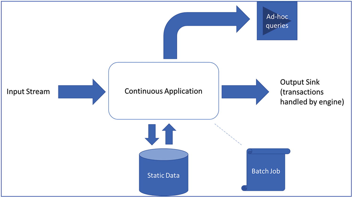
Continuous application reference architecture
Apache Spark in Azure Databricks
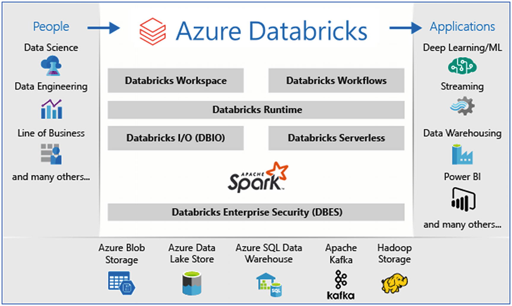
Azure Databricks ecosystem
Fully managed Spark clusters, which are created in seconds
Clusters can autoscale, depending on the load
Interactive workspace for exploration and visualization
A unified platform to host all the Spark-based applications
Instant access to the latest Spark features released by Databricks
Secured data integration capabilities built to integrate with major data sources in Azure and external sources
Integration with BI tools like PowerBI and Azure data storages like SQL Data Warehouse, Cosmos DB, Data Lake Storage, and Blob storage
Provides enterprise-level security by integrating with Azure Active Directory, role-based access controls (RBACs) for fine-grained user permission, and enterprise-grade SLAs
Exercise: Sentiment Analysis of Streaming Data Using Azure Databricks
By now, the basic concepts of Apache Spark and Databricks have been discussed. Let’s understand how to process streaming data with an Apache Spark Databricks cluster, with the help of an exercise. This exercise is about performing sentiment analysis on the Twitter data using Azure Databricks in real time.
- 1.
Event Hub: for data ingestion
- 2.
Azure Databricks: for real-time stream processing
- 3.
Cognitive services: for text analytics
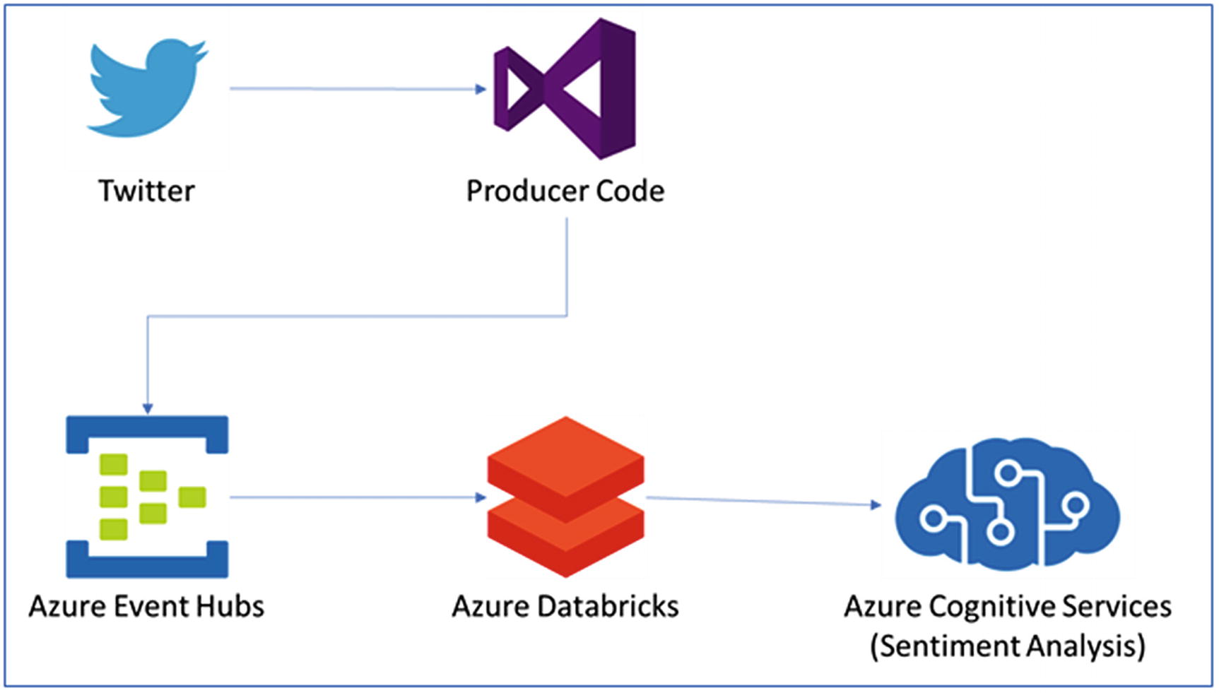
Solution architecture for Twitter sentiment analytics
- 1.
Create an Azure Databricks workspace.
- 2.
Create a Spark cluster in Azure Databricks.
- 3.
Create a Twitter app to access streaming data.
- 4.
Create an Event Hub instance.
- 5.
Create a client application to fetch Twitter data to push to Event Hub.
- 6.
Read tweets from Event Hubs in Azure Databricks.
- 7.
Perform sentiment analytics using Azure cognitive services API.
- 1.
In the Azure portal, create an Azure Databricks workspace by selecting Create a resource ➤ Data + Analytics ➤ Azure Databricks.
- 2.To create the Azure Databricks service, provide the required details, which are:
Workspace name
Subscription
Resource group
Location
Pricing tier
- 3.
Select create, and create the Azure Databricks service
- 1.
In the Azure portal, go to the Databricks workspace and select launch workspace.
- 2.
Webpage will be redirected to a new portal; select New Cluster.
- 3.In the New Cluster page, provide the following details:
- a.
Name of the cluster
- b.
Choose Databricks runtime as 6.0 or higher.
- c.
Select the cluster worker & driver node size from the given list.
- d.
Create the cluster.
- a.
- 1.
Go to https://developer.twitter.com/en/apps and create a developer account. After the developer account is created, there will be an option to create a Twitter app.
- 2.
On the create an application page, provide the required details like the purpose for creating this application and basic information on the usage of the application (Figure 6-10).
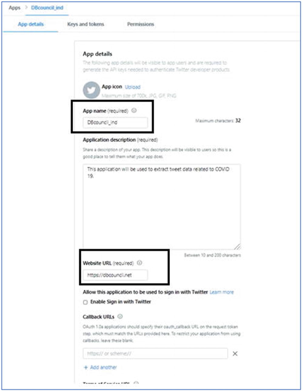
Twitter app details
- 3.
Once the application is created, go to the Keys and tokens tab. Generate the Access token and access token secret. Copy the values of customer API keys, Access token, and Access token secret (Figure 6-11).
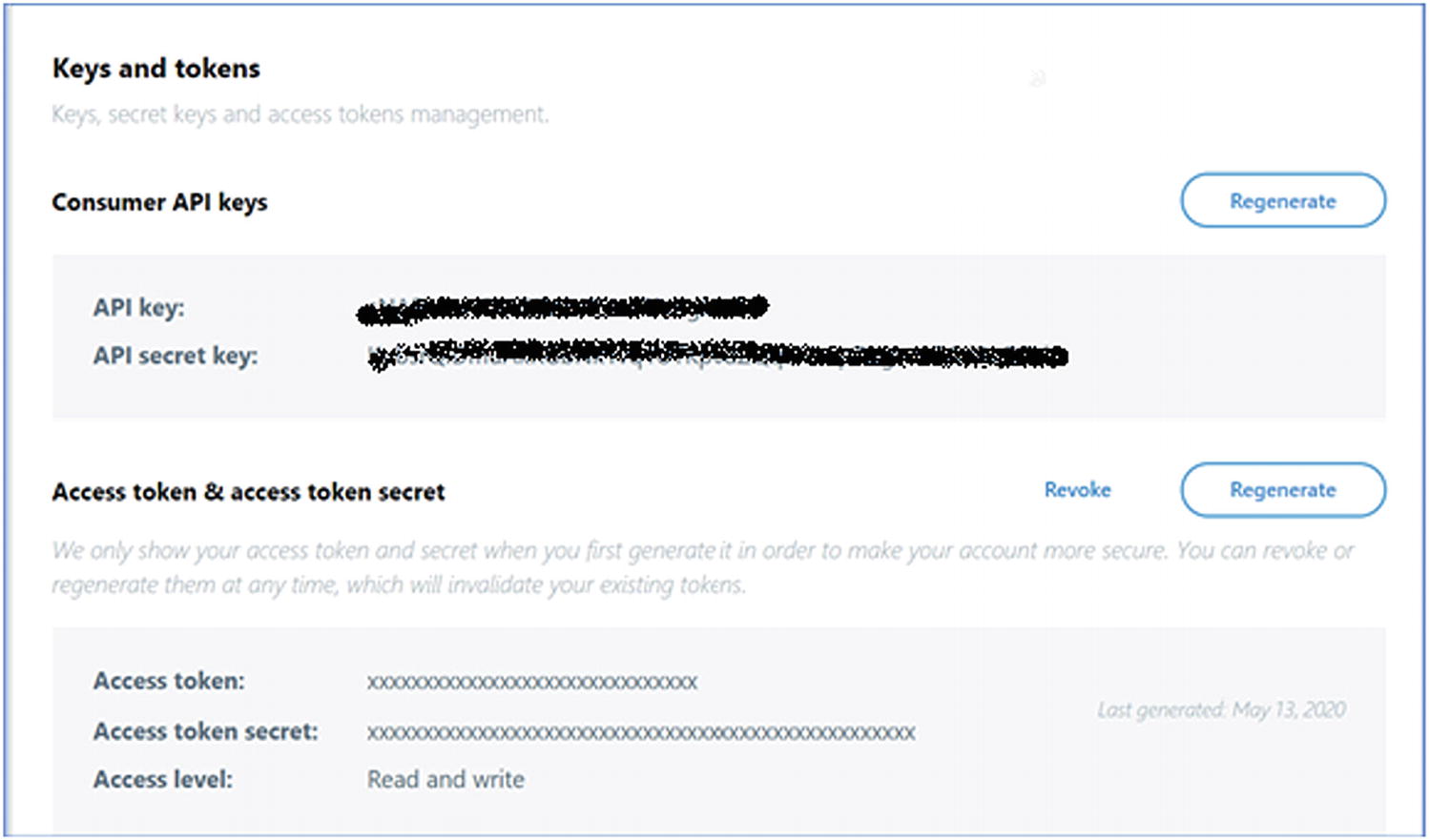
Twitter app keys and tokens
- 1.
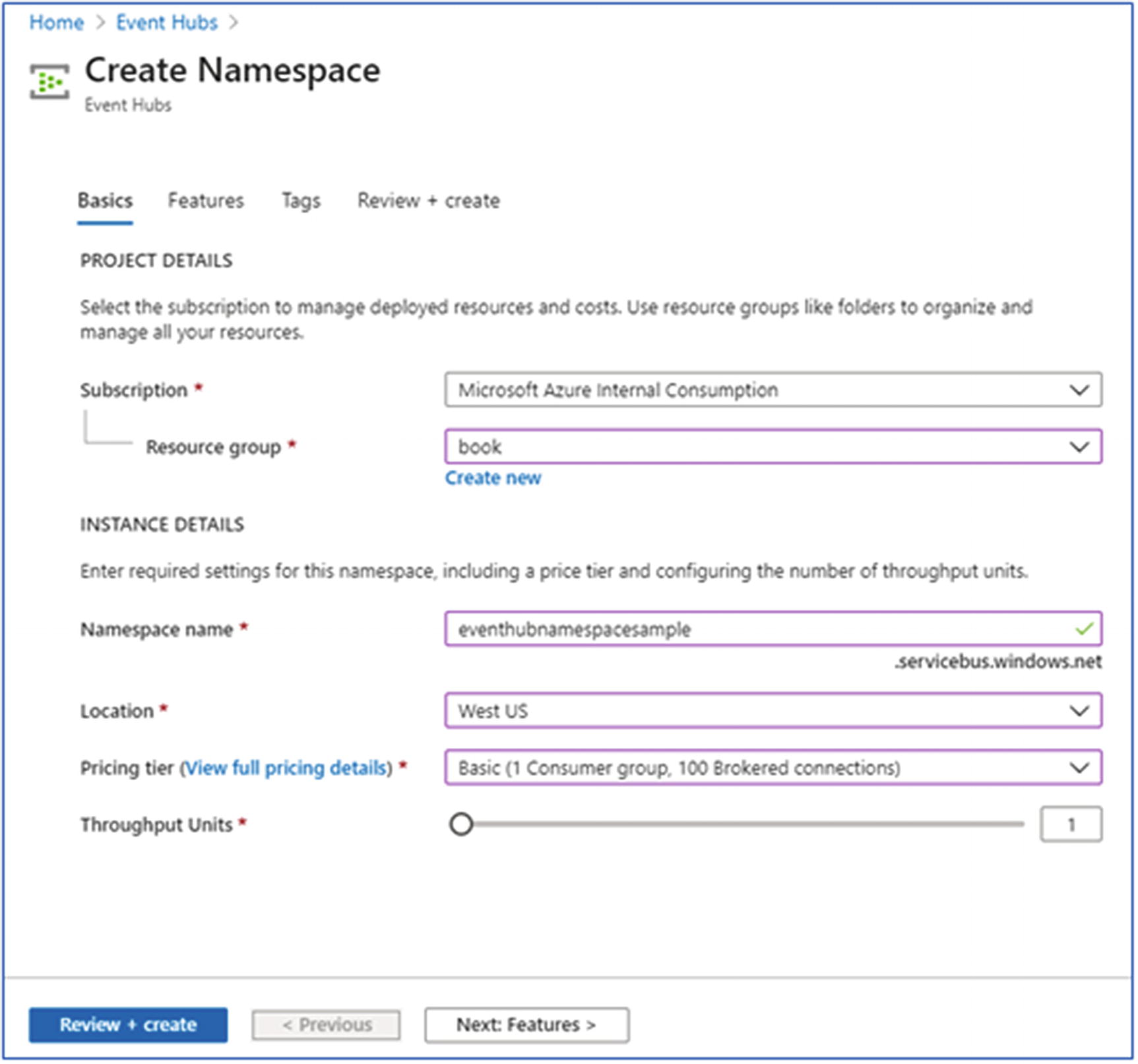
In the Azure portal, select Event Hub and create a Namespace.
- 2.Provide the following details (Figure 6-12):
- a.
Select the subscription.
- b.
Select the resource group or create a new resource group.
- c.
Provide the name of the Namespace.
- d.
Select the location of the Namespace.
- e.
Choose the Pricing tier, which could either Basic or Standard.
- f.
Provide the Throughput units settings: default is 1.
- g.
Click the Review + create button.
- a.
Create Event Hub instance
- 3.Once the Namespace is created, create an Event Hub:
- a.
On the Event Hub namespace, select the Event Hub under Entities.
- b.
Click the + button to add new Event Hub
- c.
Type a name for the Event Hub and click create.
- a.
- 1.
Create a Java application that will fetch the tweets from Twitter using the Twitter APIs, and then send the tweets to Event Hub.
- 2.
The sample project is available at GitHub at https://github.com/Apress/data-lakes-analytics-on-ms-azure/tree/master/Twitter-EventHubApp.
- 3.
In the project, Maven-based libraries have been used to connect to Twitter and Event Hub.
- 4.
A Java class named SendTweetsToEventHub.java has been created; it reads the tweets from Twitter and sends them to Event Hub on a continuous real-time basis.
- 5.
Refer to the project on GitHub and execute the project after passing the relevant configurations of Twitter and Event Hub (refer to the project file).
- 6.Once you run the code, the output displayed will be something like Figure 6-13.
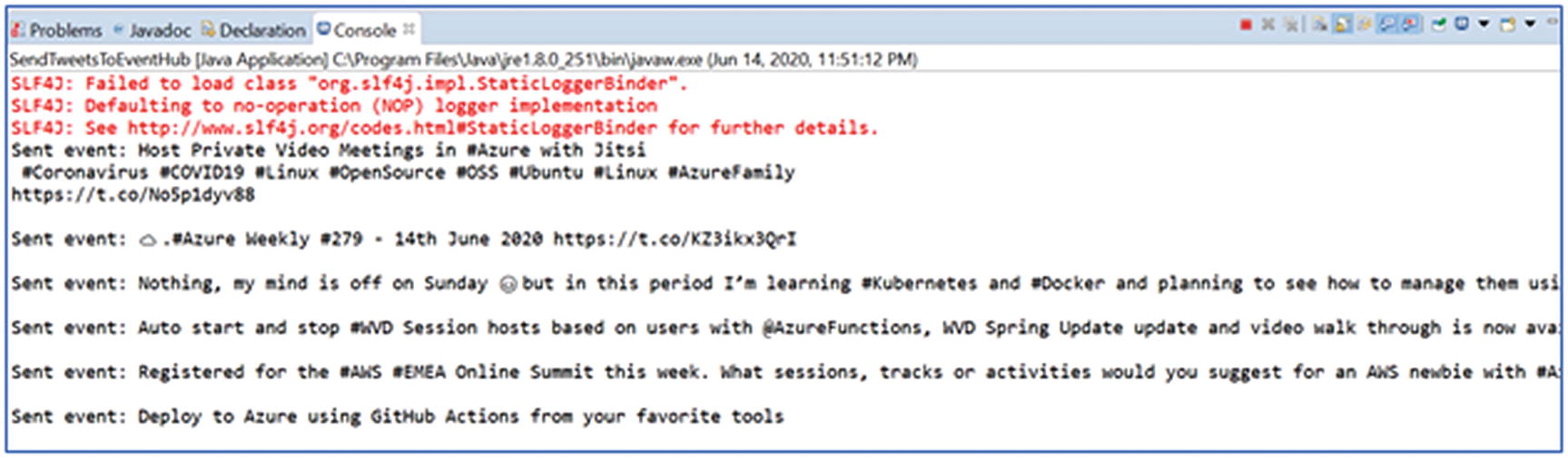 Figure 6-13
Client application output console
- 1.
Install the Event Hub library in the Spark cluster.
- 2.
In the Azure Databricks workspace, select the Clusters and choose the Spark cluster created earlier.
- 3.
Within that, select the Libraries and click Install New.
- 4.In the New library page, select source as Maven and enter the following coordinates:
Spark Event Hubs connector - com.microsoft.azure: azure-eventhubs-Spark_2.11:2.3.12
- 5.
Click Install/
- 6.
Create a Notebook in Spark named AnalyzeTweetsFromEventHub with Notebook type as Scala.
- 7.
In the Notebook (Figure 6-14), tweets from Event Hub will be ready and cognitive services APIs will be called to perform sentiment analysis on the tweets.
- 8.The notebook will return output that will display text and sentiment value; the sentiment value will be in a range of 0 to 1. A value close to 1 suggests positive response, while one near to 0 represents negative sentiments.
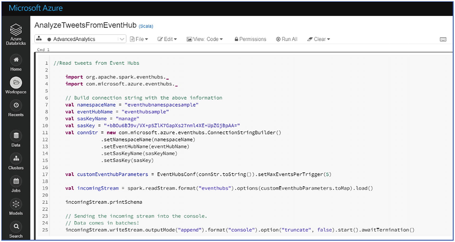 Figure 6-14
Create Event Hub instance
The preceding exercise will provide hands-on experience with an Apache Spark on Databricks cluster. Now, let’s discuss the serverless offering called Azure Stream Analytics on Microsoft Azure for real-time data processing.
Stream Analytics
- 1.
Inputs
- 2.
Functions
- 3.
Query
- 4.
Output
Inputs – Stream analytics can accept inputs from streaming platforms like Event Hubs and IoT Hubs, and from Blob storage as well. Event Hubs and IoT Hubs have been discussed in the earlier chapters. Let’s discuss when Blob storage will be used as an input to stream an analytics engine. Blob storage is generally for keeping offline data; but for a log analytics scenario, data can be picked from Blob storage as data streams. This can help to process a large number of log files using stream analytics.
Another important data input is reference data. Reference data can be used to make joins in the query to generate results that are more refined and relevant to the use case. Reference data can be picked from Azure SQL DB or an SQL managed instance or Blob storage.
- 1.
JavaScript user-defined functions
- 2.
JavaScript user-defined aggregates
- 3.
Azure ML service
- 4.
Azure ML Studio
These functions can be called in the query section to perform certain operations that are outside the standard SQL query language.
Query – The SQL query is written under this section, which processes the input data and generates the output. For real-time processing, there are a few common windowing scenarios like sliding window, tumbling window, or hopping window. There are geospatial scenarios like identifying distance between two points, geofencing, and fleet management, etc., which can be done natively with the help of functions available in a stream analytics job. Scenarios like transaction fraud or identifying any anomaly in the data can be done by invoking Azure ML service or ML Studio functions in the query.
- 1.
Data storage for batch mode processing
- 2.
Real-time dashboards and end-user notification
- 3.
Automation to kick off workflow
Data storage for batch mode – For this purpose, stream analytics output can be stored in Azure Blob storage, Azure Data Lake Storage, Azure SQL DB, MI, etc. After the data is stored in the storage layer, it can be further processed with Apache Spark on HDInsight, Databricks platform, or Synapse analytics platform, etc.
Real-time dashboards and end user notification – Stream analytics output can also land directly to power BI, Tableau, etc. for real-time dashboards. For end-user notifications, this output can land in Cosmos DB. Scenarios like the stock market, where users have to be to buy or sell stocks, or currency rate change that happens in real time and has to be notified to the traders, can be managed efficiently.
Automation to kick-off workflow – For automation to kick off workflow, Event Hubs can be used as an output or directly invoke Azure functions for performing operations like emailing a user or executing certain batch files, etc.
Exercise: Sentiment Analysis on Streaming Data Using Stream Analytics
Let’s see how a stream analytics job can be created to process the streaming data.
- 1.
Data Ingestion: Create Event Hub and ingest event data using an application
- 2.Prep and Train:
- a.
Create stream analytics job and extract the Covid-19 related tweets
- b.
Create R script for sentiment analytics using Azure ML studio
- c.
Invoke R script in stream analytics job to extract the sentiments
- a.
- 3.
Model and Serve: Show the data in Power BI and Cosmos DB
Data ingestion was done into Event Hubs using an application to extract Twitter events. In this chapter, the remaining steps to perform the sentiment analytics under Prep and Train will be performed.
- 1.
In the Azure portal, create a stream analytics job.
- 2.
Name the job and specify subscription, resource group, and location.
- 3.
Choose the Hosting environment as Cloud for deploying the service on Azure.
- 4.
Select Create.
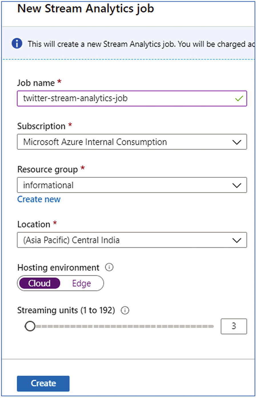
Create stream analytics instance
- 1.
Open the stream analytics; select Inputs from the menu.
- 2.
Click Add Stream Input and fill in the required details like Input Alias, Subscription, namespace, name, policy name, and compression type.
- 3.
Leave the remaining field as default and save.
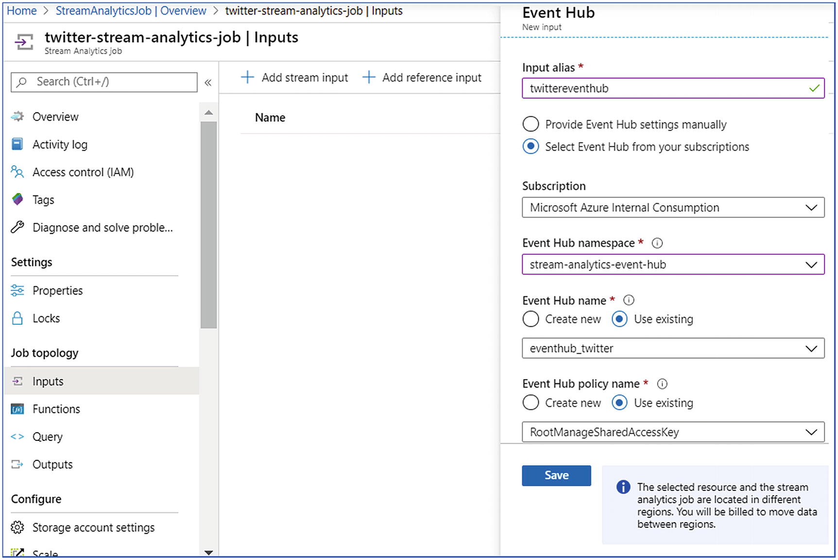
Stream analytics—input
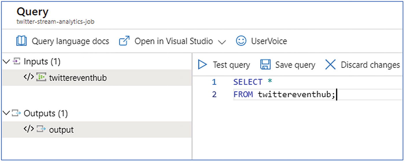
Stream analytics—query
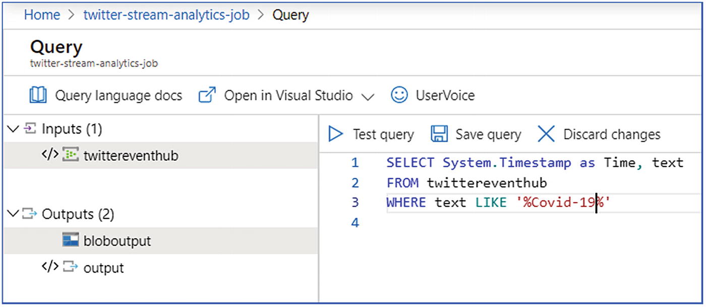
Stream analytics—query
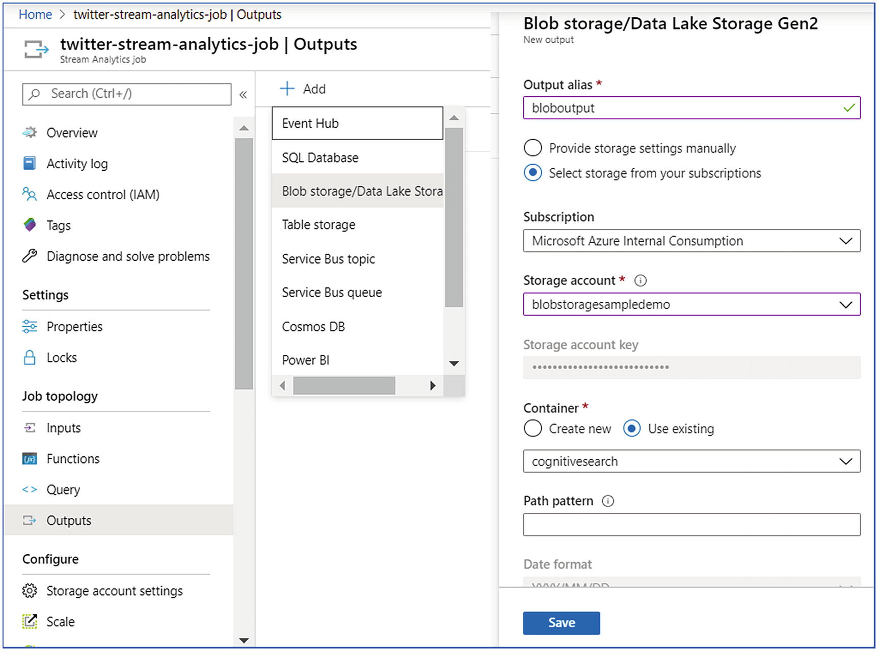
Stream analytics—outputs
Once the job is ready, you can start the stream analytics job and analyze the incoming tweets on a periodic basis.
- 1.
Create ML workspace and go to Cortana Intelligence Gallery, choose the predictive sentiment analytics model and click Open in Studio.
- 2.
Sign in to go to the workspace. Select a location.
- 3.
At the bottom of the page, click the Run icon.
- 4.
Once the process runs successfully, select Deploy Web Service.
- 5.
Click the Test button to validate the sentiment analytics model. Provide text input such as “WHO has declared coronavirus as a pandemic.”
- 6.
The service will return a sentiment (positive, neutral, or negative) with a probability.
- 7.
Now click the Excel 2010 or earlier workbook link to download an Excel workbook. This workbook contains the API key and the URL that are required later to create a function in Azure Stream Analytics.
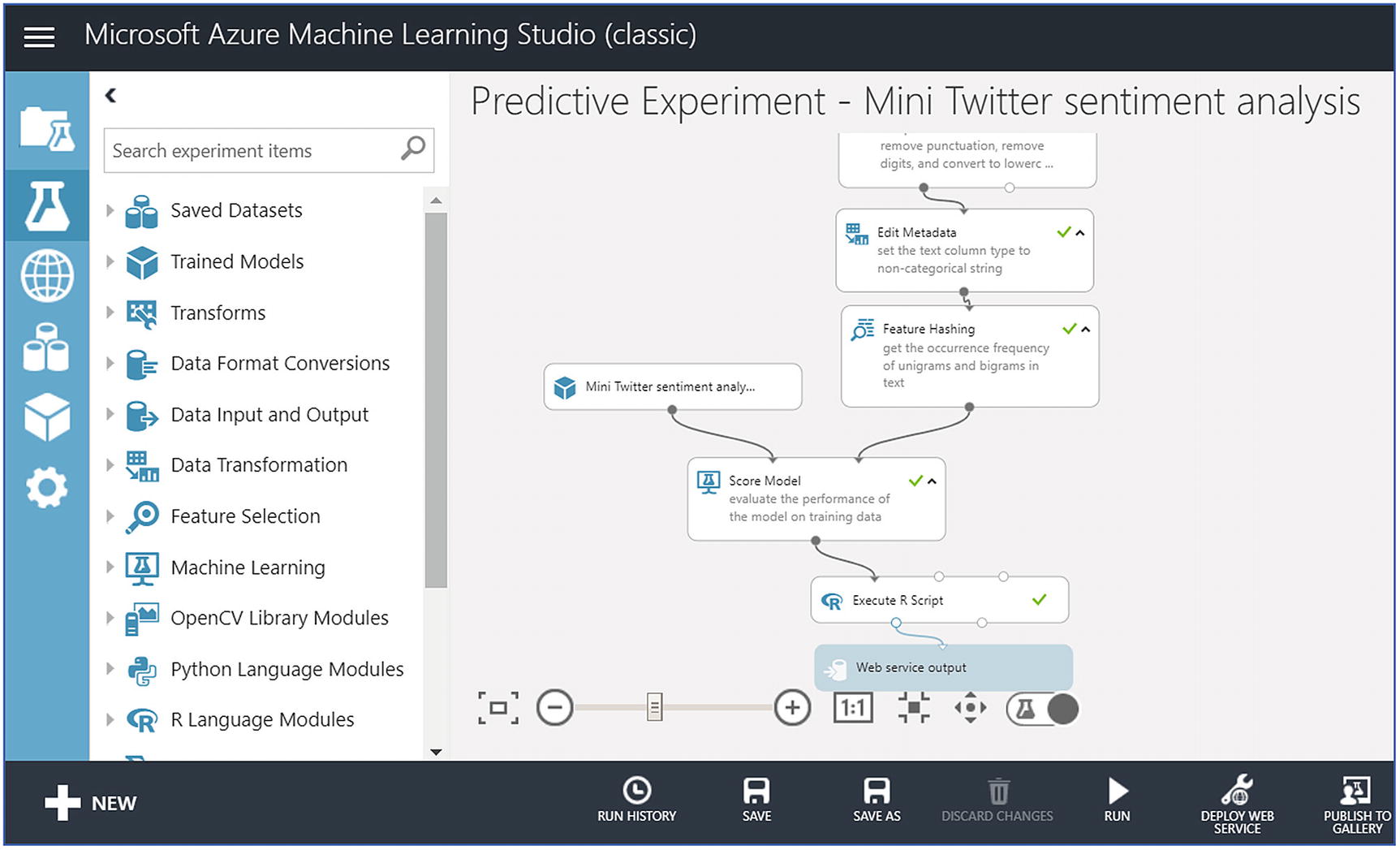
Azure Machine Learning Studio for predictive sentiment analytics
- 1.
Go to your stream analytics job and choose Functions, then click Add and choose AzureML
- 2.
Provide the required details like Functional Alias, URL, and Key. URL and Key are the same that you copied in the previous step.
- 3.
Click Save.
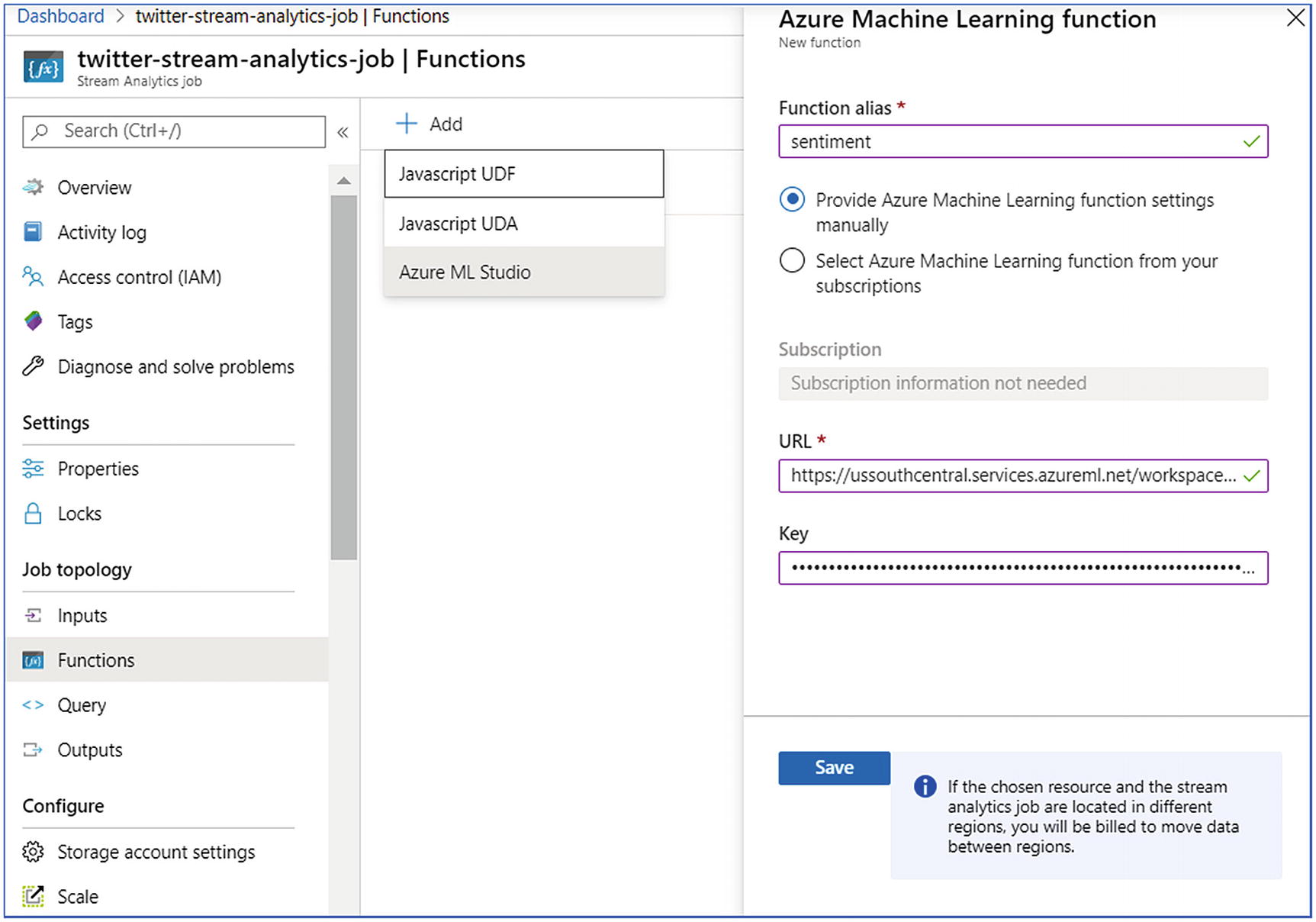
Azure Stream Analytics—user-defined function
- 1.
Under Job Topology, click the Query box.
- 2.
Enter the following query:
WITH sentimentdata AS (SELECT text, sentiment(text) as resultFROM twittereventhub)SELECT text, result.[Score]INTO bloboutputFROM sentimentdata - 3.
The preceding query invokes the sentiment function so as to perform sentiment analysis on each tweet in the Event Hub.
- 4.
Click Save query (Figure 6-22).
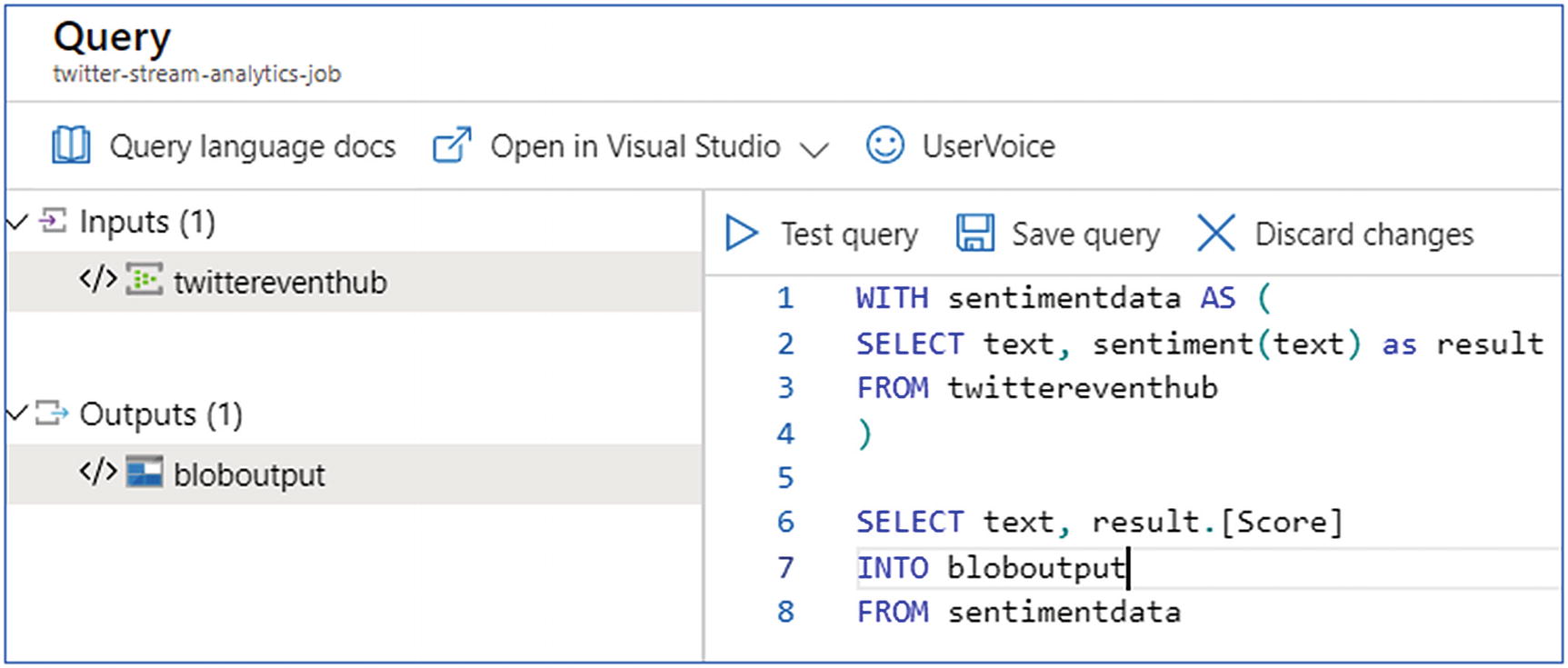
Azure Stream Analytics—query
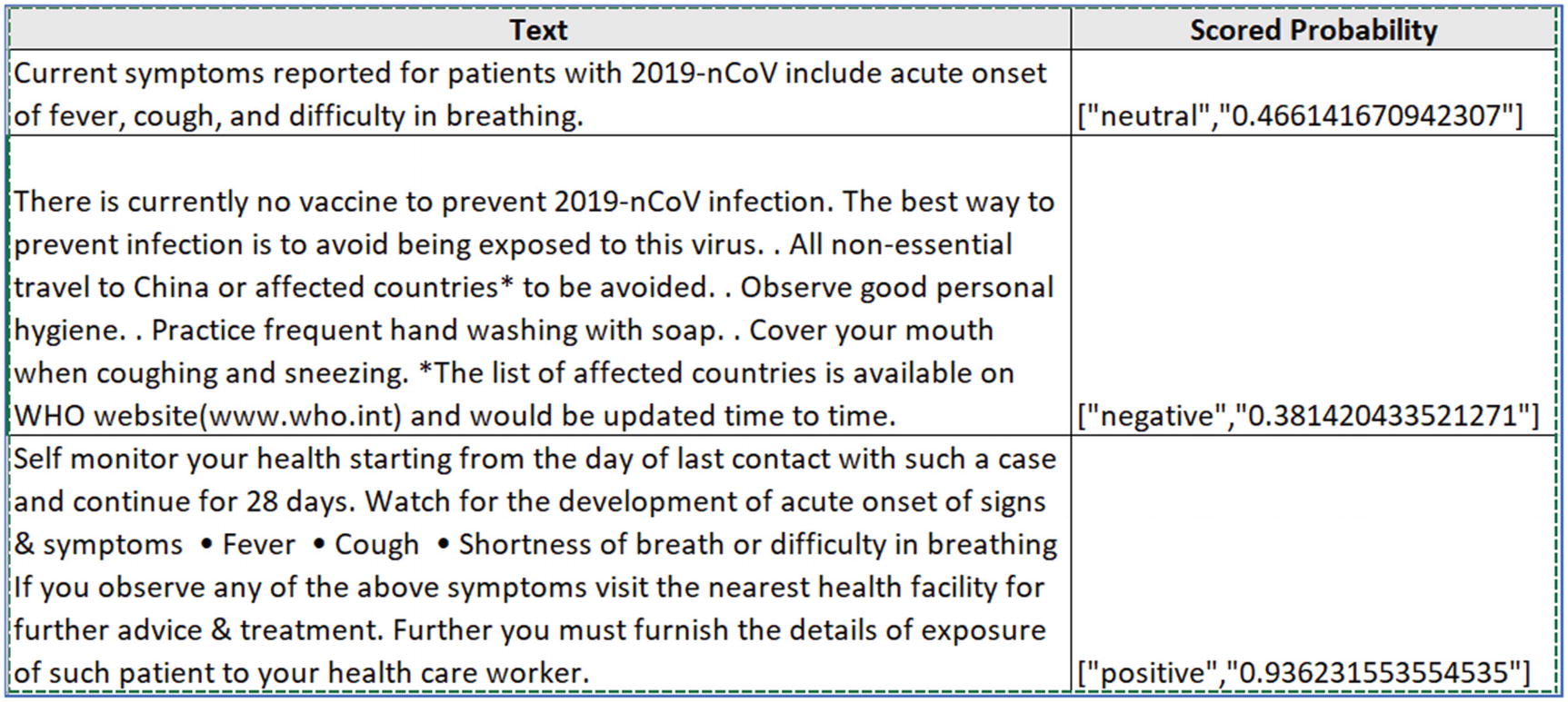
Azure Stream Analytics—query output
This output can be projected directly to Power BI or stored in Azure SQL DB or any storage, as per the use case. This is further discussed in Chapter 8.
In summary, Azure Databricks and Azure Stream Analytics are widely used solutions to process real-time data. However, data prep concepts also call for data cleansing, data transformation, data reduction etc. In the preceding section, the discussion was around stream processing. For real-time processing, especially when the response must be real time, typical data preparation steps can’t be afforded as it can induce latency. Only streaming data is processed or joined with multiple datasets or APIs, to cater to the target use cases. Data preparation techniques are followed during batch mode processing. There, the size of data is massive; data is of disparate types and all the data must be crunched together to derive a specific outcome. Let’s discuss processing batch mode data in detail in the next section.
Process Batch Mode Data
Batch mode data processing is a widely used scenario. Real-time data processing deals with millions of streams hitting the server in milliseconds, and the data processing must be done in real time. However, batch mode data processing deals with data coming from disparate applications, and the processing can be done at regular intervals or on-demand. In the recent past, lots of innovation has happened in this space. A decade ago, the majority of the solutions were based on monolithic applications built on top of structured data stores like SQL Server and Oracle, etc. Then, the only solution to process the batch data was by building enterprise data warehouses.
Enterprise Data Warehouse
- 1.
Build centralized operational data stores using ETL tools.
- 2.
Understand KPIs and build data models.
- 3.
Build a caching layer using OLAP platforms to precalculate KPIs.
- 4.
Consume these KPIs to build dashboards.
In 2010, newer types of data stores built on NoSQL technologies were introduced. Then, analyzing large data of NoSQL technologies using Hadoop ecosystem used to be done.
Further to that, there was an evolution in application architectures from monolithic to SOA and now microservices, which promoted use of polyglot technologies. This is when the tipping point occurred; there was data of multiple types getting generated from a single application. Moreover, there were multiple independent LOB applications running in silos. Similarly, CRM applications and ERP applications generated lots of data, but no system was talking to each other.
With the help of big data technologies, this data was analyzed to an extent. Technologies like Apache Spark or other Hadoop-based solutions helped to analyze massive amount of data to produce meaningful output. The public cloud further accelerated the adoption of these solutions, and analyzing this large and disparate data became easier. This was called data lake analytics.
Data Lake Analytics
Data lake analytics
The general rule of thumb is to analyze structured data with MPP architecture-based solutions like Azure Synapse analytics (Formerly known as Azure SQL DW) and unstructured and semistructured data with Hadoop-based distributed solutions like Apache Spark or Databricks., etc. However, Hadoop-based technologies can analyze structured data as well.
Let’s discuss how the world of both enterprise data warehouse and data lake analytics is changing into modern data warehouse and advanced data lake analytics, respectively. Moreover, let’s understand the key drivers that influence the decision to choose between the modern data warehouse and advanced data lake analytics.
Modern Data Warehouse
Modern data warehouse architecture
As discussed earlier, with various types of applications working in silos, it’s difficult to invest in an enterprise data warehouse running on MPP and then build another analytics platform running on Hadoop. Moreover, technical staff working on such technologies are expensive and scarce. Organizations prefer technologies that are cost effective, easier to learn, can bring data on a centralized platform, and they can leverage existing technical staff to manage these solutions. Therefore, it was necessary to build such platforms that can manage any kind of data. As shown in Figure 6-25, a modern data warehouse can manage any kind of data, and it can be a central solution to fulfill organization-wide needs.
Recently, Microsoft launched a technology solution on Azure called Synapse Analytics. This was formerly called, Azure Data Warehouse, which was built on MPP architecture. With Azure Synapse Analytics, not only structured but semistructured and unstructured data can also be analyzed. It supports both MPP SQL DW and distributed platform Apache Spark; and for dashboarding, Pipelines for ELT/ETL operations and Power BI can be easily integrated in the platform. Synapse analytics will be discussed in more detail in Chapter 8.
Exercise: ELT Using Azure Data Factory and Azure Databricks
Let’s discuss data preparation with the help of the following exercise to extract, load, and transform (ELT) data by using Azure Data Factory and Azure Databricks.
In this exercise we will learn about performing ELT operations using Azure Databricks. The data is read from a remote file system through Azure Data Factory, stored in Azure Data Lake Storage Gen2, and further processed in Azure Databricks.
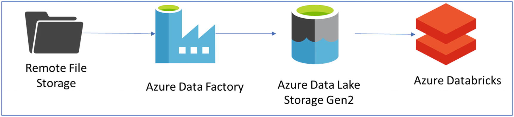
Architecture for the ELT exercise
- 1.
Azure Data Factory
- 2.
Azure Data Lake Storage (Gen2)
- 3.
Azure Databricks
- 1.
Create an Azure Databricks workspace.
- 2.
Create a Spark cluster in Azure Databricks.
- 3.
Create an Azure Data Lake Storage Gen2 account.
- 4.
Create an Azure Data Factory.
- 5.
Create a Notebook in Azure Databricks to read data from Azure Data Lake Storage and perform ELT.
- 6.
Create a pipeline in Azure Data Factory to copy data from a remote file system to Azure Data Lake Storage and then invoke Databricks notebook to perform ELT on the data.
Step 1 and step 2 to create an Azure Databricks workspace and Databricks cluster are the same as mentioned in the previous exercise.
- 1.
In the Azure portal, create an Azure Databricks workspace by selecting Create a resource ➤ Storage ➤ Storage Account.
- 2.To create the Azure Databricks service, provide the required details (Figure 6-27), which are:
Subscription
Resource group
Storage account name
Location
Performance
Account kind
Replication
Access tier
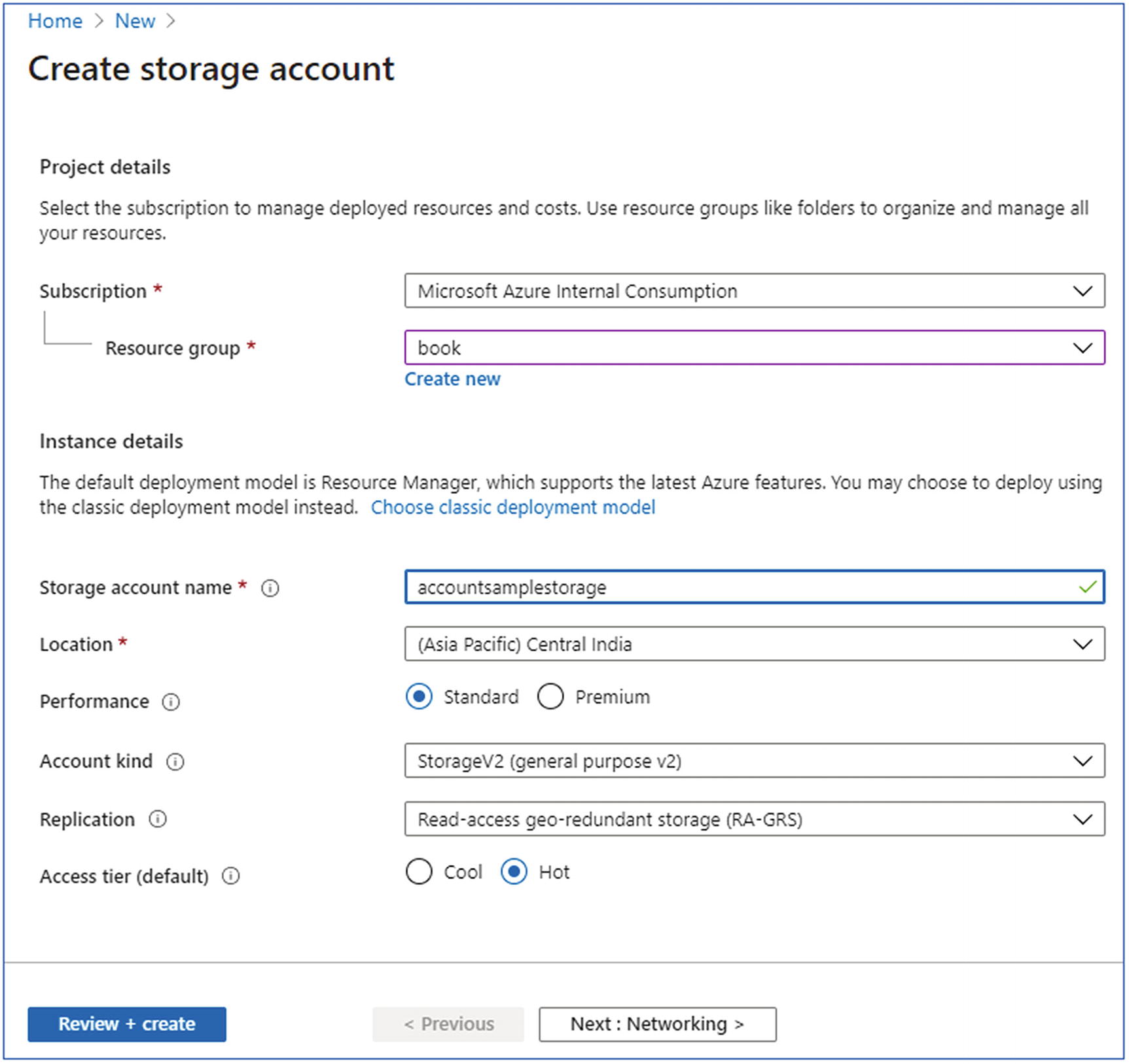
Create storage account
- 3.
Next is to enable the hierarchical namespace under the Advanced tab (Figure 6-28).
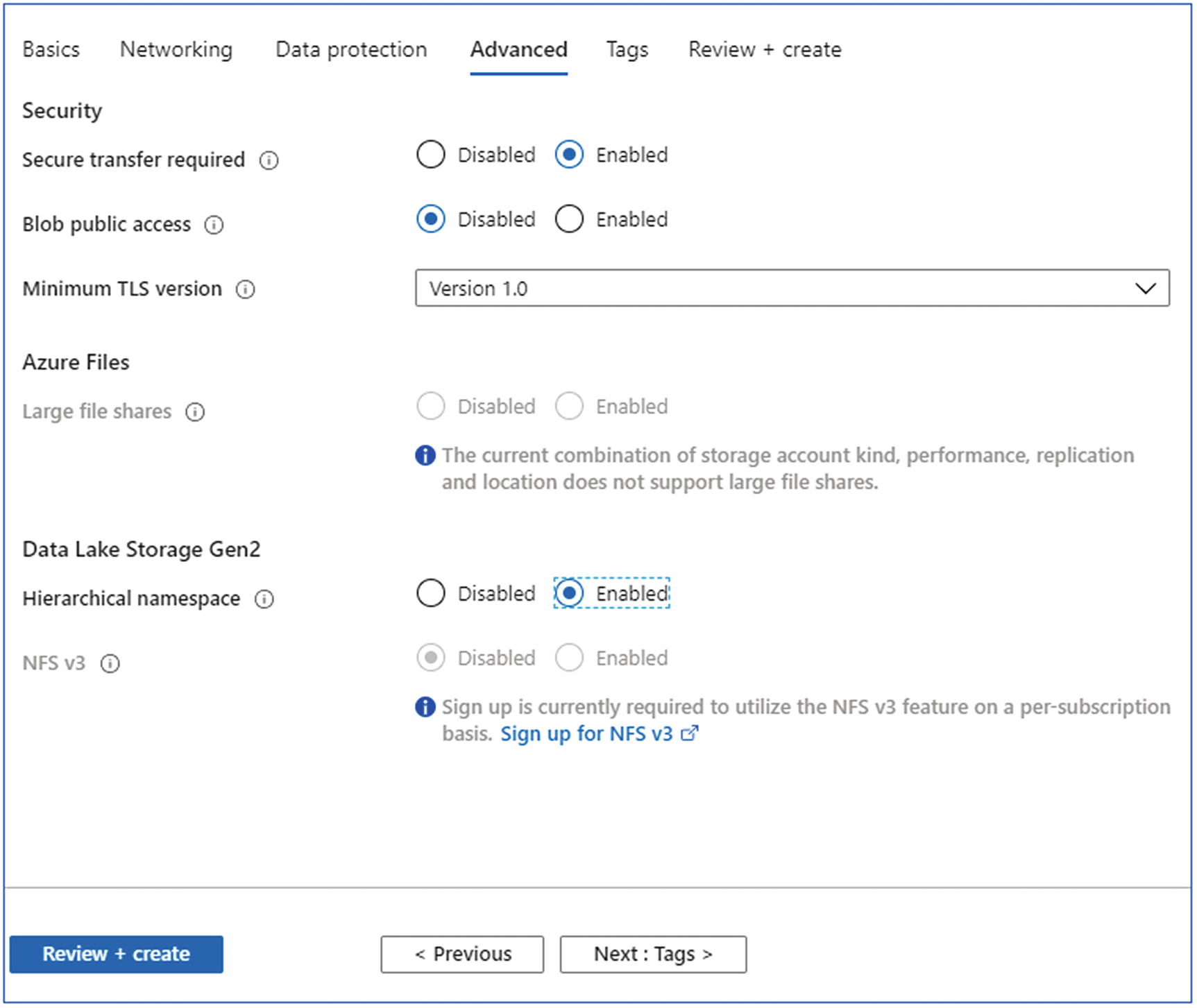
Create storage account—advanced
- 4.
Click the Review + create button to create the storage account.
- 1.
In the Azure portal, create an Azure Databricks workspace by selecting Create a resource ➤ Analytics ➤ Data Factory.
- 2.To create the Azure Databricks service, provide the required details, which are:
Name
Version
Subscription
Resource group
Location
Enable Git
- 3.
Press Create button to create
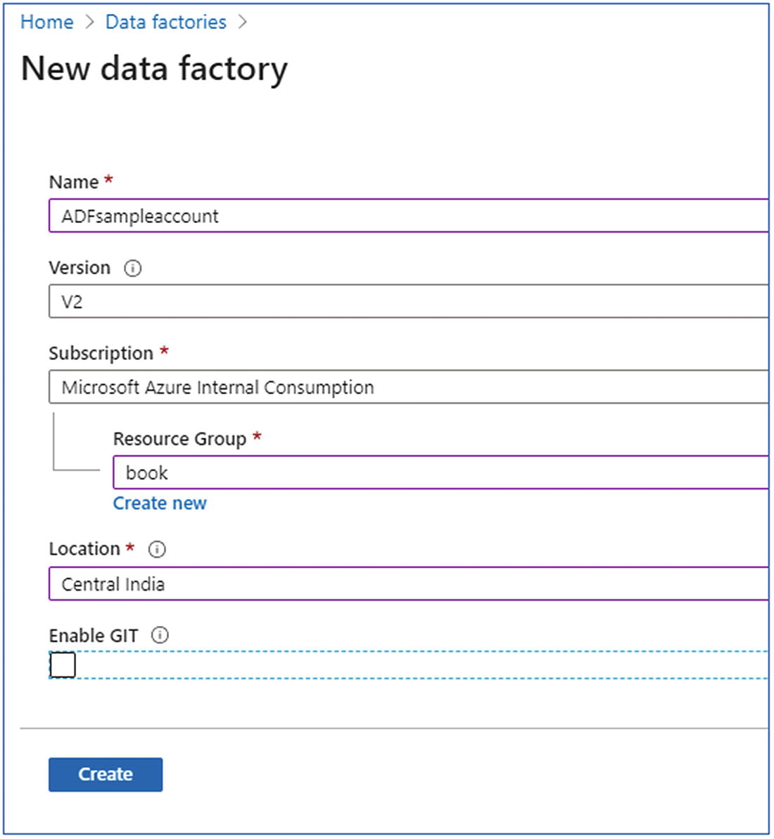
Create data factory
- 1.
Open the Azure Databricks workspace and create a Scala notebook.
- 2.The notebook is used to perform the following operations:
- a.
Connect to ADLS Gen2 storage using the keys.
- b.
Read csv data from the Storage
- c.
Load CSV data into the Spark SQL delta table.
- d.
Perform insert into the delta table.
- e.
Perform aggregation on the data.
- f.
Save the aggregated data back to ADLS Gen2.
- a.
- 3.
The sample notebook is available at https://github.com/Apress/data-lakes-analytics-on-ms-azure/blob/master/ETLDataLake/Notebooks/Perform%20ETL%20On%20ADLS(Gen2)%20DataSet.scala
- 1.
Go to the Azure Data Factory instance created in an earlier step and click Author and monitor.
- 2.
In the Data Factory UI, create a new pipeline.
- 3.This pipeline is intended to perform the following operations:
- a.
Copy data from remote SFTP location to Azure Data Lake Storage Gen2.
- b.
Invoke the Databricks notebooks created earlier to perform ELT operations on the data.
- a.
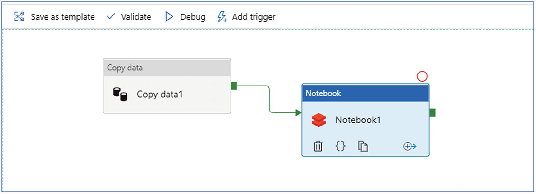
- 4.
The process looks like Figure 6-30.
Create Azure Data Factory
- 5.
To build the preceding pipeline, first you need to use a Copy Data activity, which can copy the data from source to sink: source being remote SFTP server and sink is Azure Data Lake Storage Gen2.
- 6.Create an SFTP-linked service (Figure 6-31) by passing the following parameters:
- a.
Name
- b.
Host
- c.
Port
- d.
Username
- e.
Password
- a.
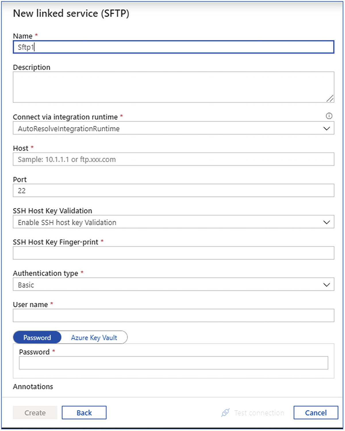
Create SFTP-linked service
- 7.Create an Azure Data Lake Storage Gen2-linked service (Figure 6-32) by passing the following parameters:
- a.
Name
- b.
Azure subscription
- c.
Storage account name
- a.
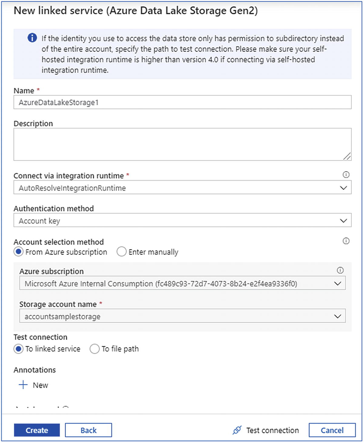
Create Azure Data Factory-linked service
- 8.Create an Azure Databricks-linked service (Figure 6-33) by passing the following parameters:
- a.
Name
- b.
Azure subscription
- c.
Databricks workspace
- d.
Cluster type
- e.
Access token
- f.
Cluster ID
- a.
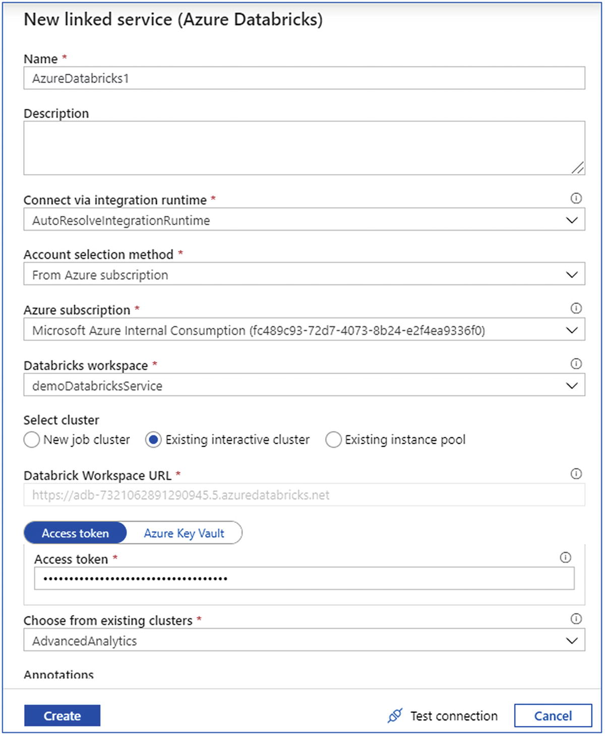
Create Azure DataBricks-linked service
- 9.Configure the copy data activity by selecting the
- a.
source dataset through the SFTP-linked service.
- b.
sink dataset through the Azure Data Lake Storage Gen2-linked service (Figure 6-34).
- a.
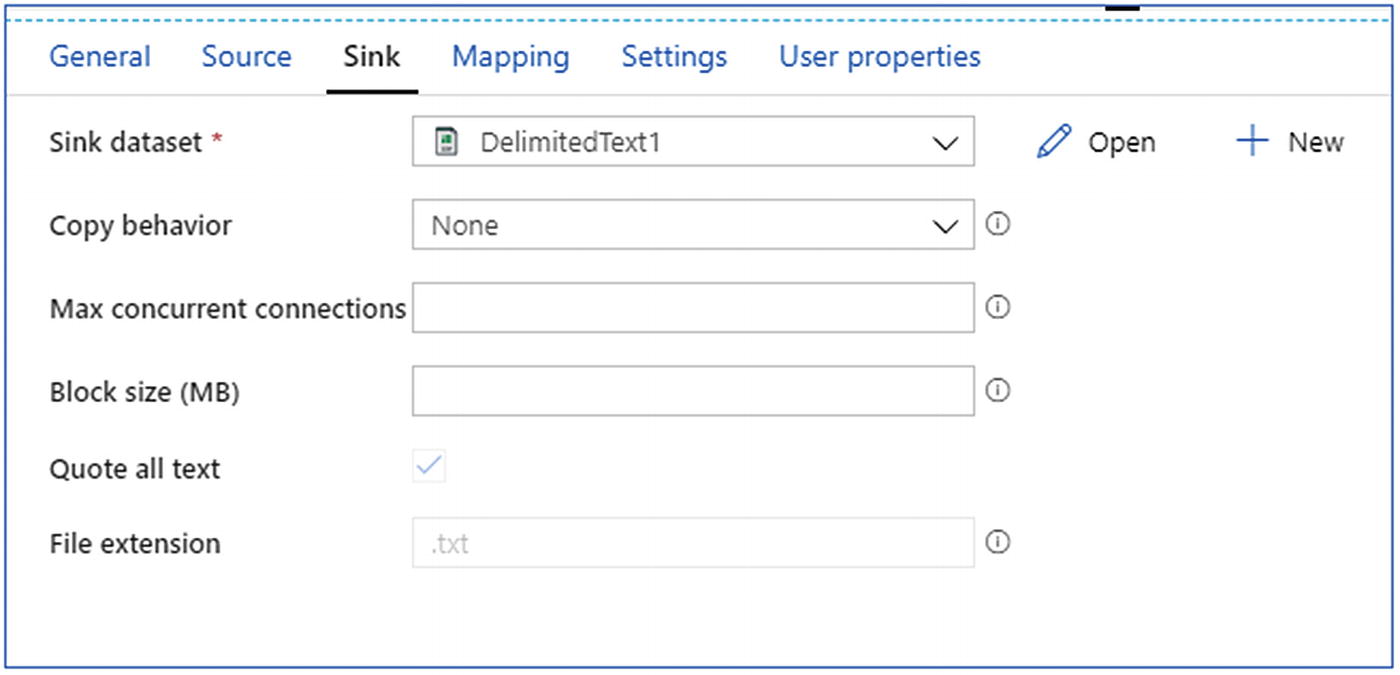
Provide the sink details
- 10.
- 11.
Once the pipeline is created, save, publish, and trigger the pipeline to monitor the results.
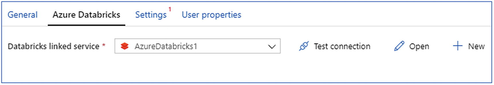
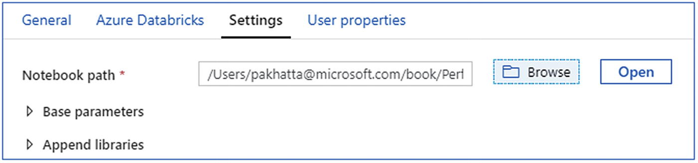
Select Azure Databricks notebook
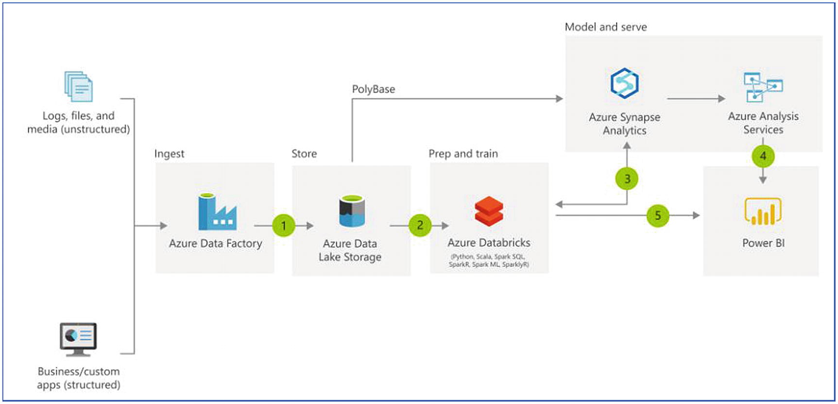
With this exercise, aggregated data is stored back on ADLS Gen2 storage, which further can be picked up under the model and serve phase. It can be picked up by Synapse Analytics using PolyBase, as shown in Figure 6-3, or directly picked up by power BI for dashboarding. In the model and serve phase, there will be an exercise on picking up this data in Synapse, caching in Analysis services, and showcasing in Power BI dashboard.
Summary
As discussed, this is the most critical phase in a data analytics solution. This phase has got lots of new innovative technologies to build cost-effective and highly efficient solutions. A decade ago, data warehouse and data mining of homogeneous data was the only way to data analytics. The solution was effective but was expensive and time consuming to set up. After moving to the cloud, the options to use MPP or distributed systems became two major options. With the transformation in the developer space, where the data was disparate, building a centralized solution was difficult. With technologies like Apache Spark, Databricks, and Azure Synapse Analytics, this journey has become easier and cost effective. Moreover, these technologies support multiple programming languages, which makes the developer ecosystem large and accessible. With the help of these solutions, nomenclature has now changed from data analytics and enterprise data warehouse to modern data warehouse. The next chapter discusses what advanced data analytics is, how the data can be prepared to train the machine learning models, and the technologies available on Azure for building advanced analytics solutions.