Steal from anywhere that resonates with inspiration or fuels your imagination… And don’t bother concealing your thievery – celebrate if you feel like it. In any case, remember what Jean-Luc Godard said: “It’s not where you take things from – it’s where you take them to.”
—Jim Jarmusch, American film director1
Obtaining a good deep neural network for most modern datasets is a difficult task. Optimizers need to traverse extraordinarily high-dimensional, jagged loss landscapes and differentiate between good and mediocre solutions using a limited set of tools. Hence, you will seldom see modern deep learning designs solving relatively well-studied problem types directly training the neural network on the data right after initialization – it’s simply too difficult to get good results feasibly by training directly from scratch.
Part of the analytical creativity embedded within deep learning design, then, is a need to turn this difficult task – modeling a complex phenomenon with a deep neural network – into a more approachable and efficient process.
In this chapter, we’ll discuss pretraining strategies and transfer learning: in essence, creatively stealing from knowledge contained in the dataset and in the weights of other models for to solve problems.
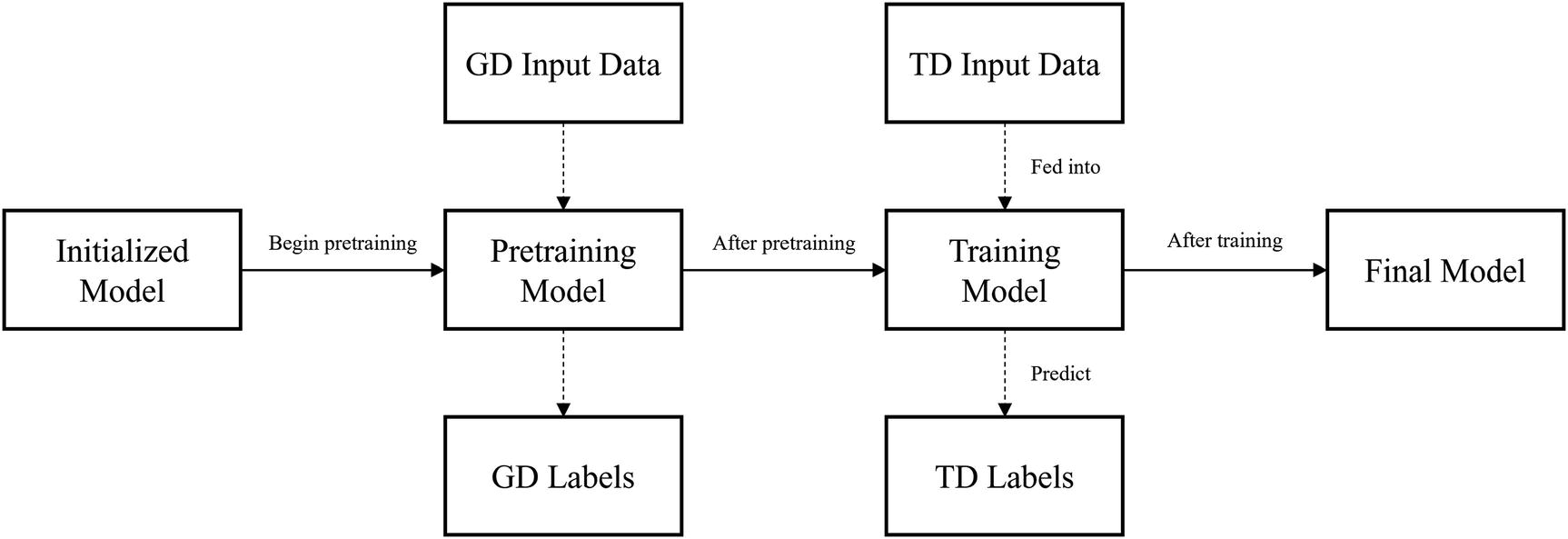
Developing Creative Training Structures
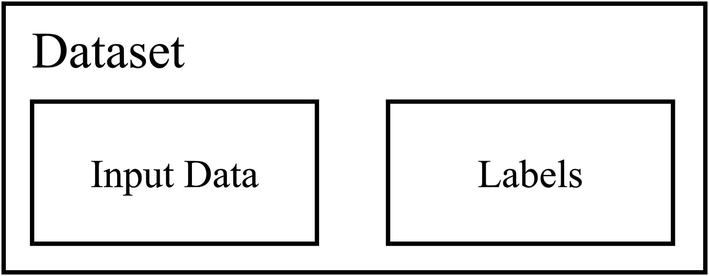
Task dataset structure
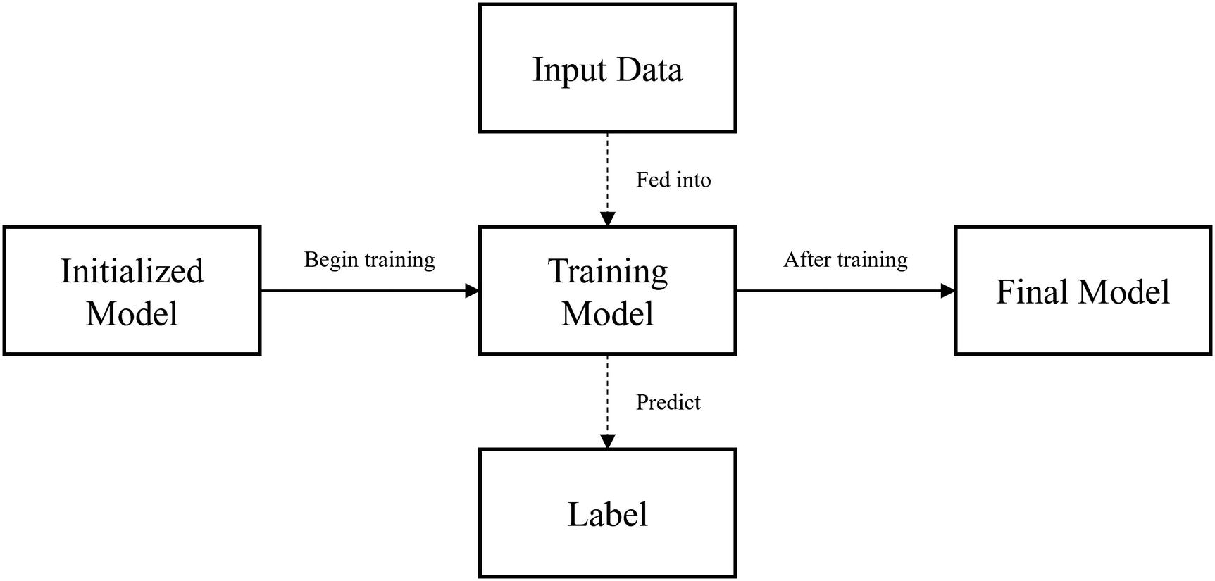
Simple training structure of initialization and training
Let’s see how we can alter this simple training structure to improve training performance more easily.
The Power of Pretraining
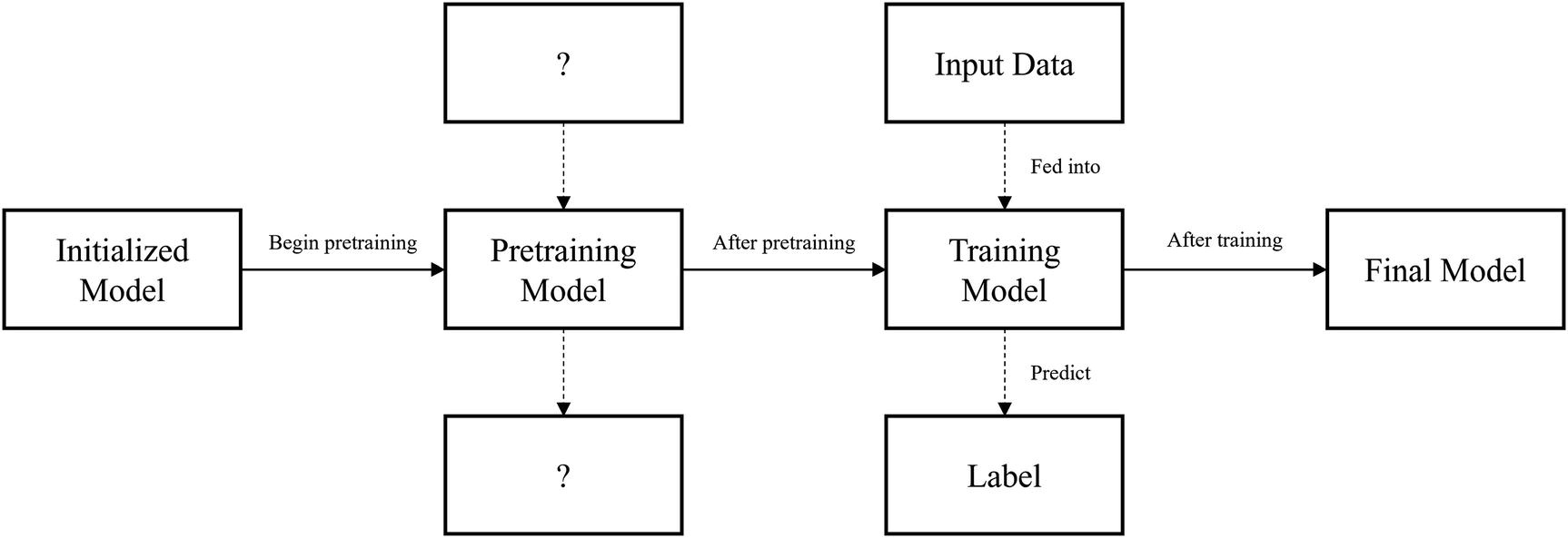
Training structure representation of pretraining
Given that we want pretraining to benefit training, pretraining should orient the model in a way that makes training “easier.” With the pretraining step, the model’s performance should be better than without pretraining. If pretraining makes model performance worse, you should reevaluate your methods of pretraining.
In pretraining, a model must be trained to perform a task different from its ultimate task of predicting the label based on the input data. This pretraining task ideally presents important “context” and skills for the ultimate task such that the model can attain better performance on that ultimate task.
Time: Pretraining can decrease the time needed for the neural network to converge to some solution.
Better metric score: The model attains a metric score higher/lower (depending on the metric) than it would have without pretraining. For instance, it attains a lower cross-entropy score or a higher accuracy.
While these are two dominant attributes of pretraining, they are the result of an underlying phenomenon: conceptually, the process of pretraining brings the optimizer “closer” to the true solution in the loss landscape.
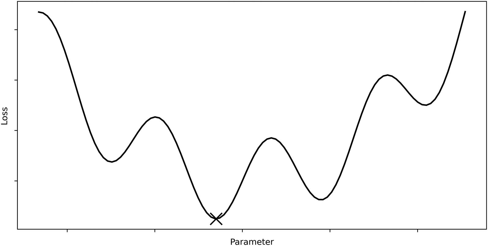
Sample loss landscape with global minima marked
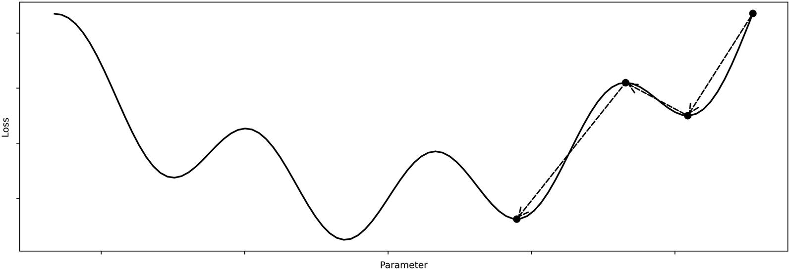
Example optimizer movement without pretraining
With pretraining, however, we’re able to get the model “closer” to the true global minimum of the loss landscape such that it converges to a more optimal solution faster, because it already begins from a place “close” to the global optimum. Correspondingly, we can use a less risky or erratically behaving optimizer because it begins from a convenient position (Figure 2-6).
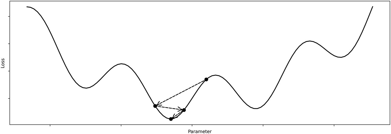
Example optimizer movement with pretraining
Note that the actual loss landscape for the pretraining task is different from that of the loss landscape of the ultimate task (as is displayed in Figure 2-6). It is not that pretraining operates within the loss landscape of the ultimate task and moves the model to a convenient position – that is just training on the task dataset, not pretraining.
Rather, in pretraining, we rely upon a similarity between the loss landscapes of the pretraining task and the ultimate task the model aims to perform. Therefore, a model that succeeds at the pretraining task should be at a generally successful location in the loss landscape for the ultimate task, from which it can further improve. This also means that pretraining may not be helpful if you believe the loss landscapes of the pretraining dataset and the task dataset are very “different.” Because the two often cannot be compared quantitatively for technical reasons, it is up to you to decide the necessity and performance boost of pretraining in a particular context.
Speed: Pretraining brings the model “closer” to a solution that the optimizer would be “satisfied with” (could converge to), because it’s already done much of the work. Moreover, most modern optimization strategies involve a decreasing learning rate. A neural network that has not had the benefit of pretraining needs to travel more (perhaps in distance, perhaps in overcoming obstacles like local minima or maxima) to near the true solution. By then, its learning rate can be expected to have decayed significantly, and it may not be able to get out of local minima. On the other hand, if a pretrained model begins already near the true solution, its learning rate begins “fresh” and undecayed; it can quickly overcome local minima that lie between it and the true solution.
Better metric scores: Pretraining reduces the quantity of obstacles between a model and the true solution. Thus, the model is more likely to converge to the true solution. Moreover, as discussed prior, the optimizer’s learning rate is more “fresh” near the true solution than an optimizer without pretraining and thus is less susceptible to being vulnerable to minor obstacles that may have tricked the optimizer without pretraining.
Next, we’ll build upon this conceptual model to discuss the intuition behind two pretraining methods: transfer learning and self-supervised learning.
Transfer Learning Intuition
Transfer learning is premised upon the idea that knowledge gained from solving one problem can be used, or transferred, in solving another problem. Usually, the knowledge derived from a more general problem is used to aid a model’s ability to address a more specific problem.
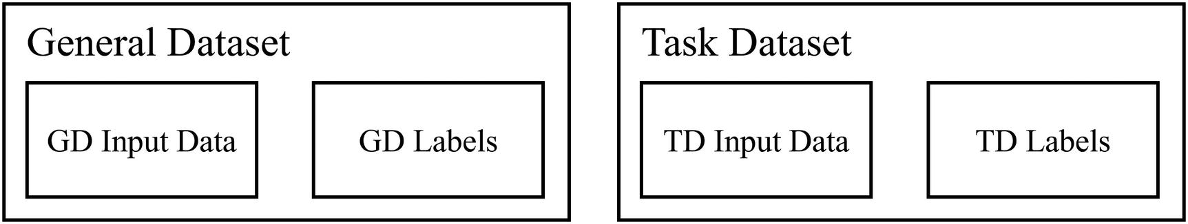
General dataset and task dataset visual representations. GD = general dataset, TD = task dataset
Training structure visual representation of transfer learning
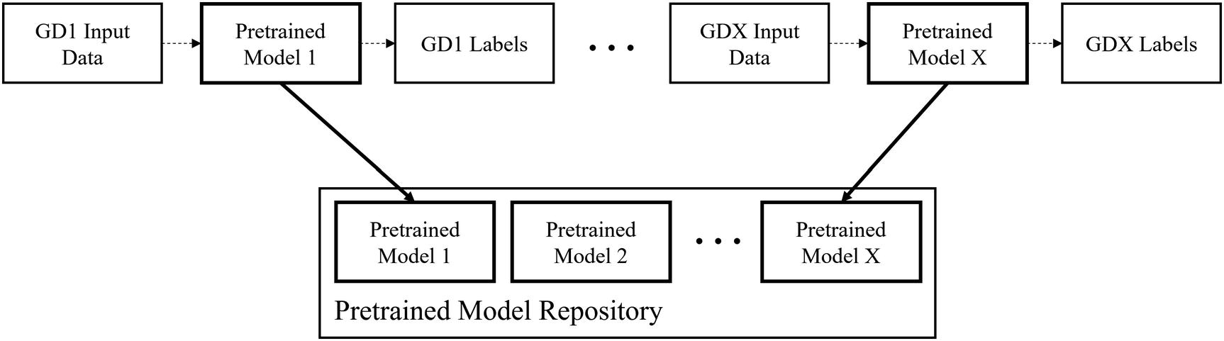
Pretrained models in a model repository. GD = general dataset. GD1, GD2, …, GDX indicate several different general datasets upon which several pretrained models are correspondingly trained. Note that in practice the relationship between general datasets and pretrained models is one to many (many pretrained models with different architectures are trained on the same general dataset)
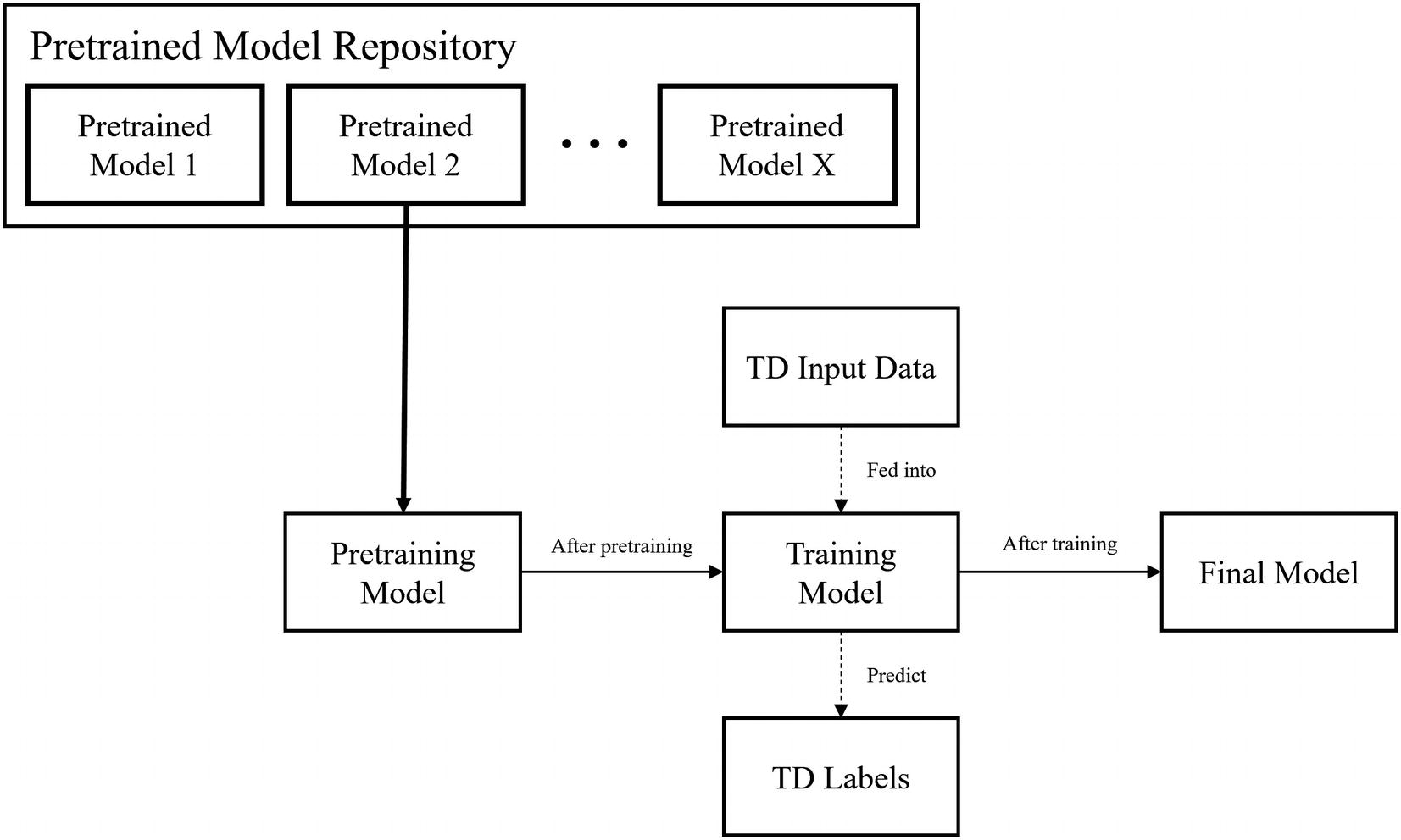
Using models from a pretrained model repository to directly begin training on the task dataset
The number of problems with which this set of pretrained models could be used vastly outnumbers the number of pretrained models in the repository. This is fine, though, because we can expect each pretrained model to be capable of being applied to a wide array of problem types, since each model is expected to possess a form of “general knowledge.”
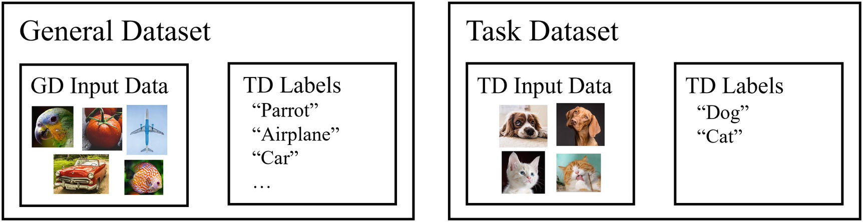
Example task dataset and general dataset
There are many edges: Edges define the shapes of the airplane, car, and fish; likewise, they are important in defining the shape of a dog or cat’s head.
Light is important: Since both datasets are two-dimensional representations of three-dimensional objects, light is important because it helps determine the shape and contour of the object.
Texture matters: Real-life objects often have similar shapes but are differentiated by the texture of their surface. Likewise, this seems to be important toward differentiating between images of dogs and cats.
A model that succeeds on the general dataset must have already adapted to and accounted for these features of the general dataset. In a sense, it “understands” how to “interpret” edges, the dynamics of light, texture, and other important qualities. All that is necessary afterward is to adapt those learned skills and representations toward a similar but more specific task.
You may ask, “why not approach task dataset directly? Why develop these auxiliary skills when the model could have developed those skills more specifically and directly for the task dataset?” Indeed, in some cases transfer learning is not a suitable choice. However, in most sufficiently difficult tasks, pretraining via transfer learning helps to set up the foundation for learning that would be difficult for the model to build by itself.
Teach the child directly to add two-digit numbers by repeatedly showing them examples (e.g., 23+49=72).
First, teach the child how to add one-digit numbers by repeatedly showing them examples (e.g., 3+9=12, 2+6=8). Then, teach the child to add two-digit numbers by repeatedly showing them examples (e.g., 23+49=72).
The latter is more likely to be a successful strategy, because the average length of the jump from knowing nothing about addition to adding one-digit numbers to adding two-digit numbers is much smaller than the average length of the jump from knowing nothing about addition to adding two-digit numbers. Transfer learning should operate by this same intuition of teaching the model a general task such that a more specific, ultimate task becomes easier to approach.
Self-Supervised Learning Intuition
Self-supervised learning follows the logic of pretraining – some sort of pretraining task is performed before training the model on the task dataset to orient it toward better attaining representations and skills needed to perform well on the ultimate task.
The difference between self-supervised learning and transfer learning is that in transfer learning, the pretraining dataset is different from the task dataset, whereas in self-supervised learning, the pretraining dataset is constructed from the input data of the task dataset. Thus, while you would need two datasets to build the complete transfer learning training structure, only one is technically needed to build the complete self-supervised learning training structure (Figure 2-12).
Here, we are using a unique definition of what a “different” dataset constitutes. If dataset A can be derived completely from dataset B (for instance, by flipping the images or changing image color), for the purposes of this concept, the two datasets are not different, even though on a technical level there are training instances in one dataset that cannot be found in the other. On the other hand, if dataset A cannot be derived completely from dataset B (for instance, deriving ImageNet from CelebA), the two datasets are different. The main focus of what constitutes “difference” here is the informational content of the dataset, not the individual specific training instances. This allows us to distinguish transfer learning and self-supervised learning.
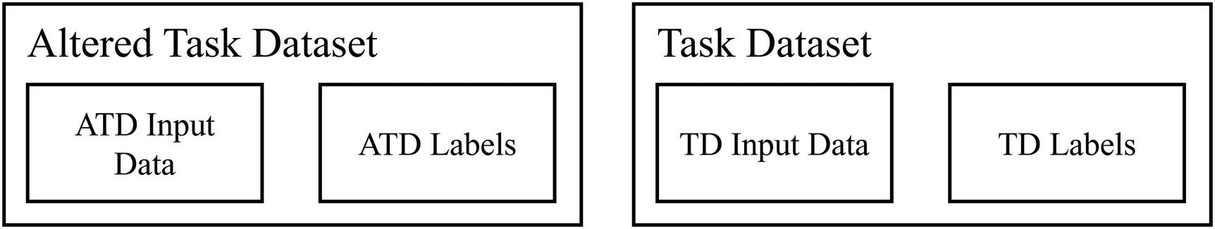
Self-supervised learning datasets. ATD = altered task dataset
It’s important to note that the altered task dataset is generally derived only from the input data of the task dataset. For instance, if a model’s task is to identify whether an image is of a dog or a cat, the altered task dataset could only be built upon the images (the input data of the task dataset), not the labels (the labels of the task dataset).
Add noise to some of your data and none to others. Train the model to classify to which data instances noise was added (this is a binary classification problem: noise/no noise). This can help the model better separate noise and data, allowing it to develop an underlying representation of what key features of the data should look like.
Add varying degrees of noise to all instances in the dataset. Train the model classify the degree of noise (this is a regression problem). For instance, if you varied the standard deviation of Gaussian noise, the model would predict the standard deviation. This not only helps the model detect if there is noise, but to what extent it exists. While this is a more difficult pretraining task, the model would be encouraged to develop sophisticated representations of key features and structures of the data.
Assume there is a dataset of colored images and color is important to the model’s ultimate task. Convert the images to grayscale and train the model to construct a colorized image from the corresponding grayscale one (this is an image-to-image task). In this case, the altered task dataset input data is the grayscale image and the labels are the colorized images. With this self-supervised pretraining exercise, the model gains an understanding of what color certain objects should be.
Assume there is a model that needs to perform the NLP (Natural Language Processing) task of text classification. Take the text samples (input data for the task dataset) and randomly hide one of the words. Train the model to predict what the hidden word is. For instance, the model would predict “cats” when given “it’s raining ____ and dogs.” This allows the model to gain an understanding of how words function in relation to each other bidirectionally – it needs to take advantage of information both before and after the hidden word. This method of self-supervised learning is commonly used in modern NLP architectures.
In each of these examples, none of the task dataset’s labels are needed – only the input data, or the x, of the task dataset is used in constructing these supervised datasets. You, as the deep learning engineer, can make some change to the task dataset input data and construct labels from that change.
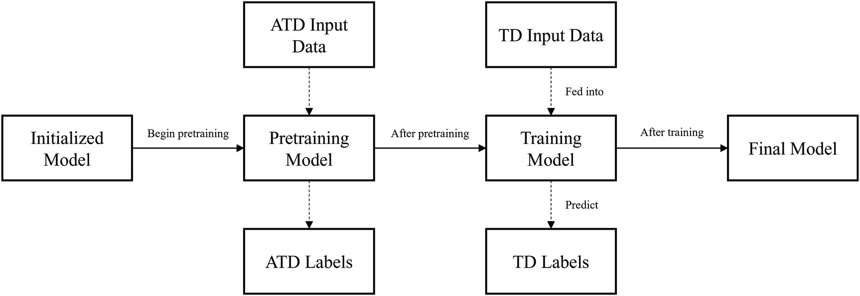
Self-supervised learning training structure
Note that in self-supervised learning (and pretraining in general), attaining a high performance metric is not the ultimate goal. In fact, if a model performs too well on the pretraining task, it may be that the pretraining task was too easy and hence did not support the growth of valuable skills and representations of data for formal training. On the other hand, if the model performs very poorly, the pretraining task may be too difficult.
It should be noted that self-supervised learning is technically unsupervised learning because we are extracting insights from the input data without any knowledge of the labels. However, self-supervised learning is a more commonly used and appropriate term: there is undoubtedly a supervised character to this sort of operation that distinguishes it from traditional unsupervised machine learning algorithms like K-means in that while the data generation (constructing altered task dataset) is technically unsupervised, the learning procedure (gradient updates, etc.) is supervised.
Self-supervised learning is also valuable because it allows us to capture valuable information without needing labels. Datamation estimates that the amount of unstructured data is increasing by 55% to 65% every year,2 and the International Data Corporation projects that 80% of data will be unstructured by 2025.3 Unstructured data is defined as data that cannot be easily fit into a standard database model. An auxiliary characteristic of unstructured data, thus, is that there are seldom corresponding labels to train massive deep learning models with. However, the logic of self-supervised learning allows us to find hidden structures in unstructured data without labels and to exploit that knowledge to solve supervised problems.
For this reason, self-supervised learning is especially valuable for training on small datasets, in which there are few labels. Pretraining via self-supervised learning can allow the model to derive important insights it may not have obtained with only the traditional training structure.
Unlike transfer learning, there is no repository of self-supervised pretrained models, because in self-supervised learning, the pretraining task must be designed based on the task dataset. However, altering task datasets for self-supervised learning is generally not difficult if you have a good grasp of programming and data flows (see Chapter 1).
Self-supervised learning … is basically learning to fill in the blanks. Basically, it’s the idea of learning to represent the world before learning a task. This is what babies and animals do. We run about the world, we learn how it works before we learn any task. Once we have good representations of the world, learning a task requires few trials and few samples.
—Yann LeCun, Chief AI Scientist at Facebook, speaking at AAAI 204
Transfer learning tends to develop “prediction skills.” That is, the weights from transfer learning are derived from the general dataset, which usually comes from a significantly different context than the task dataset (topic/content-wise). Much of the value of transfer learning is in the predictive skills it develops – learning how to recognize edges, to look for texture, to process color, etc. rather than actual knowledge of the content or topic of the dataset.
Self-supervised learning tends to develop “world-representing knowledge.” It builds the fundamental representations of the “world,” or context, that the model will need to understand to perform well on the task dataset. The actual skill of predicting whether – for instance – noise was or was not added to a training instance may not be of much use, but the process of deriving that skill requires gaining an understanding of the data “world.” Self-supervised learning allows for the model to get a glimpse into building fundamental representations and “feeling around” for the dataset’s content and topics.
Of course, this is not to suggest that transfer learning does not develop world-representing knowledge or that self-supervised learning does not develop important skills. Rather, these are the root-level “spirits” or “characters” of transfer learning and self-supervised learning that can be used to guide intuition and what to expect from either method.
You may notice that we have been exploring these concepts through relatively fluid and artistic descriptors and ideas – “extracting insights,” “developing representations,” “world-representing.” While a textbook may attempt to formulate these ideas in equations and mathematical relationships, the truth is that even the most modern deep learning knowledge cannot fully explain and understand the depth of neural network behavior. Having an intuitive grasp of how neural networks function and “learn” – even if it is not mathematically rigorous – is valuable toward successful and efficient design.
Next, we will explore practical concepts in pretraining to understand how to manipulate neural network architectures for the implementation of transfer learning and self-supervised learning.
Transfer Learning Practical Theory
Previously, we discussed conceptual frameworks to gain an intuitive understanding for what transfer learning is, what it does, and how it operates. However, because there are many “hidden” considerations when implementing transfer learning, in this section we will explore the more practical aspect of theory – concepts and ideas to aid your implementation of transfer learning.
The purpose of this section is not to provide specific code or discuss examples (that will be left to the next section), but instead to provide an introduction to important concepts for implementing pretraining, like the structure of pretrained models and how pretrained models are organized in Keras.
Transfer Learning Models and Model Structure
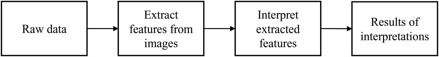
Conceptual components of an image-based pretrained model
Feature extraction serves the purpose of assembling information into meaningful observations, like identifying and amplifying (or reducing) the presence of certain edges, shapes, or color patterns. A well-tuned feature extraction component is able to identify and amplify characteristics that are relevant to the problem. For instance, if the problem is to classify various grayscale images of shapes, the feature extraction component must be highly capable at detecting and amplifying the shape of edges.
Feature interpretation interprets the compiled extracted features to make a final judgment about the image. It takes in extracted information regarding the features of the image and can perform comparisons and other complex analyses across various regions of the image. A well-tuned feature interpretation component is able to effectively aggregate and make sense of extracted features in relation to the target output.
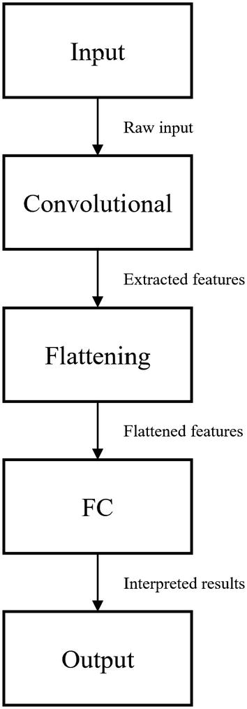
The practical components of an image-based pretrained model
- 1.
The raw input is passed into the convolutional component for feature extraction.
- 2.
The convolutional component of the pretrained model takes in the raw input and performs convolutions, pooling, and other image-processing layers to extract features from the image. It then passes the extracted features into the flattening component.
- 3.
The flattening component takes in the two-dimensional (spatially, not counting color depth), since the convolutional component performs operations that take in and output data of image form. Flattening converts the two-dimensional extracted features into one-dimensional data so that the fully connected layer can operate upon the features.
- 4.
The fully connected component, also known as the “top” or the “head” of the neural network, takes in the one-dimensional flattened data containing the information from the extracted features. After interpreting the extracted features through a series of fully connected layers (and other corresponding layers, like activations, dropout, etc.), the fully connected layer outputs the output of the neural network.
We’ll talk more about certain architectures in depth in later chapters, but here we’ll do a very quick overview of important models.
In Keras, pretrained models are arranged into modules from which that model and related functions can be found within keras.applications.module_name. For instance, if you wanted to find the pretrained model and processing functions relating to the InceptionV3 model, you would find it in keras.applications.inception_v3. In addition to the pretrained model object, these modules often contain processing functions to apply to your data or the model output. We will see how these processing functions work in relation to the model soon.
The ImageNet Dataset
ImageNet is one of the most important datasets in image recognition. Professor Fei-Fei Li began working on ImageNet at Princeton in early 2007. Throughout the development of neural network applications in the image domain, ImageNet has been a core dataset upon which new methods and designs were conceived, tested, and reinvented.
Hypothetical example branch of WordNet hierarchy organization
The ImageNet project was inspired by two important needs in computer vision research. The first was the need to establish a clear North Star problem in computer vision… Second, there was a critical need for more data to enable more generalizable machine learning methods. Ever since the birth of the digital era and the availability of web-scale data exchanges, researchers in these fields have been working hard to design more and more sophisticated algorithms to index, retrieve, organize and annotate multimedia data. But good research requires good resources…The convergence of these two intellectual reasons motivated us to build ImageNet.
—ImageNet Research Team5
The ImageNet Large Scale Visual Recognition Challenge ran from 2010 to 2017 and was instrumental to the development of image-processing deep learning work. Hence, many of the pretrained models available in Keras/TensorFlow and other deep learning frameworks are pretrained on the ImageNet dataset. Models pretrained on the ImageNet dataset have developed skills to recognize edges, textures, and other attributes of images of three-dimensional spaces and objects .
ResNet
The ResNet architectures , or residual neural networks, were introduced in 2015. ResNet won first place in the 2015 ImageNet challenge, obtaining a 3.57% error on the test dataset. The ResNet uses residual connections, or skip connections, which are connections between layers that skip over at least one intermediate layer. We’ll explore these sorts of designs and strategies in neural network architectures in later chapters.
Keras/TensorFlow offers several different versions of the ResNet architecture: ResNet50, ResNet101, ResNet152, ResNet50V2, ResNet101V2, and ResNet152V2. The number after the “ResNet” (e.g., the “50” in “ResNet50”) indicates the number of layers in it. Thus, ResNet152V2 has more layers than ResNet101V2.
ResNetV1 adds more nonlinearities than ResNetV2. The V2 architecture thus allows for a more direct and clear path for data flow throughout the network.
ResNetV1 passes the data through a convolutional layer before batch normalization and an activation layer, whereas ResNetV2 passes data through the batch normalization and activation layers before the convolutional layer (reversed).
ResNet50: keras.applications.resnet50.ResNet50()
ResNet101: keras.applications.resnet.ResNet101()
ResNet152: keras.applications.resnet50.ResNet152()
ResNet50V2: keras.applications.resnet_v2.ResNet50V2()
ResNet101V2: keras.applications.resnet_v2.ResNet101V2()
ResNet152V2: keras.applications.resnet_v2.ResNet152V2()
We will explore how to use the architecture given the model object later .
InceptionV3
The 2015 InceptionV3 model is a popular model from the Inception family of models, using a module/cell-based structure in which certain sets of layers are repeated. Inception networks are more computationally efficient by reducing the number of parameters necessary and limiting the memory and resources needed to be consumed. InceptionV3 was designed primarily with a focus on minimizing computational cost, whereas ResNet focuses on maximizing accuracy.
You can find the InceptionV3 model architecture at keras.applications.inception_v3.InceptionV3().
Inspired by the high performance of ResNet, the Inception-ResNet architecture uses a hybrid module by incorporating residuals. Correspondingly, Inception-ResNet generally has a low computational cost with high performance.
You can find the Inception-ResNetV2 architecture at keras.applications.inception_resnet_v2.InceptionVResNet2().
For more specific and technical discussion on residual connections, cell-based structures, and the InceptionV3 architecture, see Chapter 6.
MobileNet
The 2017 MobileNet models are designed to perform well on mobile phone deep learning applications. MobileNets use depth-wise separable convolutions, which are convolutions that apply not only spatially but also depth-wise. MobileNet has more parameters than Inception but less than ResNet; correspondingly, MobileNet has been generally observed to perform worse than ResNet but better than Inception.
When we compare models (e.g., “MobileNet vs. ResNet”), keep in mind that we are referring to the complete family of architectures. Most models have architectures of different versions and depths. When comparing model families, we are referring to architectures of comparable versions and layers.
Keras/TensorFlow offers four versions of MobileNet, MobileNetV1, MobileNetV2, MobileNetV3Small, and MobileNetV3Large. MobileNetV2, like MobileNetV1, uses depth-wise separable convolutions but also introduces linear bottlenecks and shortcut connections between bottlenecks. MobileNetV2 can effectively extract features for object detection and segmentation and generally performs faster at achieving the same performance as MobileNetV1. MobileNetV3Small and MobileNetV3Large are MobileNet architectures designated for low-resource and high-resource consumption scenarios, derived from Neural Architecture Search algorithms (we will discuss Neural Architecture Search and other methods in later chapters).
MobileNetV1: keras.applications.mobilenet.MobileNet()
MobileNetV2: keras.applications.mobilenet_v2.MobileNetV2()
MobileNetV3Small: keras.applications.MobileNetV3Small()
MobileNetV3Large: keras.applications.MobileNetV3Large()
EfficientNet
Deep convolutional neural networks have continually been growing larger in an attempt to be more powerful. Exactly how this enlargement is performed, however, has varied. Some approaches increase the resolution of the image by increasing the number of pixels in the image handled by the network. Others increase the depth of the network by adding more layers or the width by increasing the number of nodes in each layer.
The 2019 EfficientNet family of models is a new approach for neural network enlargement via compound scaling, in which the resolution, depth, and width of the network are equally scaled. By using this scaling method upon a small, base model named EfficientNetB0, seven compound-scaled architectures were generated, named EfficientNetB1, EfficientNetB2, …, EfficientNetB7 as the magnitude of scaling increases. The EfficientNet family of models is both powerful and efficient, both computationally and time-wise. Compound scaling allows EfficientNet to improve upon the performance of models like MobileNet and ResNet on the ImageNet dataset.
EfficientNetB0: keras.applications.efficientnet.EfficientNetB0()
EfficientNetB1: keras.applications.efficientnet.EfficientNetB1()
EfficientNetB2: keras.applications.efficientnet.EfficientNetB2()
…
EfficientNetB6: keras.applications.efficientnet.EfficientNetB6()
EfficientNetB7: keras.applications.efficientnet.EfficientNetB7()
Find a more specific and technical discussion of EfficientNet in a Chapter 6 case study .
Other Models
Keras/TensorFlow offers a host of other pretrained models in keras.applications. To view them, refer to the TensorFlow documentation, which not only provides information on usage, parameters, and methods but also includes the links to each pretrained model’s corresponding paper: www.tensorflow.org/api_docs/python/tf/keras/applications. Later in this chapter, we will also cover how to convert PyTorch models into Keras/TensorFlow models to take advantage of PyTorch’s library of pretrained models.
Changing Pretrained Model Architectures
To change pretrained model architectures , usually only the pretrained model’s convolutional component is transferred. Recall that transfer learning is primarily concerned with transferring the skills learned from one general dataset for application in a specific task dataset. Because the task dataset is different from the general dataset, while a model operating on the task dataset would still benefit from the feature-extracting skills transferred via transfer learning, it would need to develop its own interpretations.
…retain the feature-extracting skills: The fundamental feature extraction capabilities that you learned as an art student are important to developing and organizing meaningful and astute observations that can be used for interpretation. Without understanding how to look at and take away observations of art (without actually interpreting them), there are no observations to serve as the basis of interpretation.
…but develop a fresh set of interpretations: Now that you have kept your feature extraction skills and have developed a set of observations (the extracted features), it wouldn’t in most contexts make sense to analyze the contemporary work through Impressionist interpretations. Rather, this new data calls for a fresh set of interpretations suited toward the context of contemporary art.
The process of transferring weights from a pretrained model to a custom model. PM = pretrained model, CM = custom model. “Updated” indicates that the corresponding component is being trained/updated in retraining
An alternative process of transferring weights from a pretrained model to a custom model in which both the pretrained model’s convolutional and FC components are transferred
An alternative process of transferring weights from a pretrained model to a custom model in which both the pretrained model’s convolutional and FC components are transferred, and new fully connected layers are added to the custom model
Although we will only explore the first method through examples, all can be implemented through tools covered in Chapter 1, like the Functional API. Models can be treated like functional layers, expressed as functions of an input. See Chapter 3 for more complex exploration into neural network architecture manipulation.
Neural Network “Top” Inclusivity
All Keras/TensorFlow pretrained models have an important parameter, named include_top, which allows us to easily implement the first method of changing pretrained model architectures for training.
Recall that the fully connected component of an image-based neural network architecture is often referred to as its “top.” Thus, if the include_top parameter is set to True, the fully connected component will be retained in the instantiated pretrained model object. On the other hand, if the include_top parameter is set to False, the fully connected component will not be retained and the instantiated pretrained model object will contain only the input and convolutional components.
It’s important to realize that when there is no top, the input image shape is more or less arbitrary (see Note) because convolutional layers do not rely upon an absolute shape. A convolutional layer can act on an image of almost any shape (see Note for the qualifier “almost”), since it simply “slides” filters over an image. On the other hand, a dense layer in the fully connected component can only act upon inputs of a certain shape. Thus, if the include_top parameter is set to True, you are also limited in the shape of your input data to whatever the shape of the data the model was pretrained on.
The input image shape is not completely arbitrary. If the image shape is too small, the image may not be large enough for the whole depth of the network to be able to be valid, since filters rely on a minimum image size. One cannot perform ten convolutions with kernel size (3,3) on a 16x16 pixel image because in the middle of the sequence the feature map will have been reduced so much that it is too small to perform convolutions on. This is likely the culprit if you are using a model architecture with a small input size that throws an error when defining the architecture.
It should also be noted that the fact that the absence of a top means the input size is somewhat arbitrary does not mean that you should be too extreme with how much you change the input shape of your image. Say, a model was trained on 512x512 pixel images and you used transfer learning by extracting the convolutional component of that model (along with its weights). If you were to train the model on 32x32 pixel images (likely with image resizing), even though the operation is technically valid, the transferred weights are rendered more or less useless because the skills in the original model were developed on more high-resolution pixel images. In short, make use of the relatively arbitrariness of image sizes with no top, but also take your freedom in image size with a grain of salt.
Layer Freezing
Layer freezing is a useful tool for the implementation of transfer learning. When a layer is “frozen,” its weights are fixed and it cannot be trained. The purpose of transfer learning is to utilize important skills the pretrained model has developed. Thus, it is common to freeze the convolutional component of the pretrained model and to train only the custom fully connected component (Figure 2-20). This way, the feature-extracting skills learned and stored in the weights of the convolutional component are kept as is, but the interpretative fully connected component is trained to best interpret the extracted features. After this, sometimes the entire network is trained for fine-tuning. This allows the convolutional component to be updated in accordance with the developed interpretations in the fully connected component. Be aware that too much fine-tuning can lead to overfitting.

A multistep layer freezing process
On a practical level, layer freezing is immensely helpful for practical success. Although it can be easy to build massive neural networks and call .fit() with increasing computational power, it remains true that it is not easy to optimize hundreds of millions (or even billions) of parameters by brute-force and achieve good performance. Layer freezing allows the neural network to focus on optimizing one segment of its architectures at a time and allows you to better use the weights gained from pretraining by restricting how much the neural network can deviate from the learned pretrained weights .
Implementing Transfer Learning
- 1.
No architecture or weight changes: An exercise in using (ImageNet) pretrained models for their original purpose – to predict what object is in an image. Also helpful for dealing with reshaping inputs and using encoding and decoding functions associated with the pretrained model module
- 2.
Transfer learning without layer freezing: Using the standard procedure of transferring the weights from the convolutional component and building a custom fully connected component, without layer freezing. Helpful for manipulating model architectures both using the Functional API and using the include_top parameter
- 3.
Transfer learning with layer freezing: Using the standard procedure of transferring the weights from the convolutional component and building a custom fully connected component, with layer freezing
We’ll also discuss how to take advantage of PyTorch’s pretrained model library by converting them into Keras/TensorFlow models.
General Implementation Structure: A Template
- 1.
Choose an appropriate model from the Keras/TensorFlow repository of pretrained models or from another source, like a pypi library offering an implementation of a pretrained model or PyTorch.
- 2.
Instantiate the model with the desired architectural settings (include or do not include top).
- 3.
Set up the model’s input and output flows such that it matches with the data. This may require using a reshaping layer, using an input layer, adding a fully connected component such that the extracted features are interpreted and outputted, some other mechanism, or some combination.
- 4.
Freeze layers, as necessary.
- 5.
Compile and fit.
- 6.
Change which layers are frozen if necessary, and compile and fit again.
It should be also noted that although in this context we are discussing image-based pretrained models, as transfer learning began its extensive development in the domain of images, the logic of a feature-extracting segment and an interpretative segment can be applied to other problem domains as well.
No Architecture or Weight Changes
If we make no changes to the architecture, we cannot adjust the input or the output of the pretrained model. Therefore, if we want to make no changes to the architecture, we must use the pretrained model for its original purpose.
The InceptionV3 model was trained on the ImageNet dataset. Thus, it takes an image of size (299,299,3) and returns an output vector with the probability the image belongs to one of 1000 classes.
Loading image of a lion
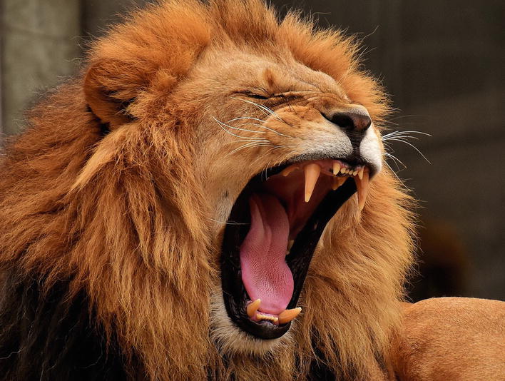
Sample image to be classified by a model architecture trained on the ImageNet dataset
The keras.layers.Input layer defines the input size and is required for constructing a neural network (or in some other form, like the input_shape parameter).
The keras.layers.experimental.preprocessing.Resizing layer resizes an image to a new shape. We can use this to reshape an image of any size to the shape (299,299,3) such that it is in the proper input shape for InceptionV3.
The keras.applications.inception_v3.InceptionV3 model is the core InceptionV3 model that can be used and manipulated in relation to the other layers.
The keras.applications.inception_v3.preprocess_input preprocesses data to be in the same format InceptionV3 was trained on. If the inputs are not preprocessed, the pretrained weights may not be suited toward the unprocessed inputs and yield inaccurate results.
Importing necessary libraries
Building input of a transfer learning neural network
The output of preprocess_layer (the result of the resized, preprocessed input data) is passed as the input to the InceptionV3 model. Note that we are making no changes to the model architecture or weights, so we set inlucde_top=True and weights='imagenet'. We can treat the model as a layer that takes in the output of a previous layer and can be passed as an input to the following layer: Inceptionv3 = InceptionV3(include_top=True, weights="imagenet")(preprocess_layer).
Note that you can set weights to None to just use the model architectures, without the pretrained weights. Although this doesn’t quite count as transfer learning, you may want to use this when the task dataset is so different from the pretraining dataset that any pretrained weights wouldn’t be of much benefit, but want to take advantage of some architecture’s characteristics, like efficiency or power.
We can create a model out of this set of layers using keras.models.Model (note that the pretrained model is treated like a layer and thus is considered an outputs layer): model = keras.models.Model(inputs=input_layer, outputs=Inceptionv3).
Running and decoding predictions for a pretrained model
Note that the model expects four-dimensional data – for example, data with shape (100,299,299,3), indicating that it consists of 100 299x299 pixel RGB colored images. Even though we are submitting an individual image for prediction, it still needs to be four-dimensional. An easy way to accomplish this is to wrap it as an element in another array with np.array([im]).
Results of InceptionV3 decoded predictions on an image of a lion
A similar process can be applied to other pretrained models available via Keras. Most Keras pretrained models have associated preprocess_input and decode_predictions functions.
Transfer Learning Without Layer Freezing
If we want to adapt the pretrained model for our own task dataset, we need to make some minimal architecture changes such that the input and the output can accommodate our dataset. This follows a very similar structure to the previous application of no architecture or weight changes.
The keras.layers.Input layer defines the input shape.
The keras.layers.Dense layer provides the neural network’s “interpretative” or “predictive” power.
The keras.layers.GlobalAveragePooling2D layer “collapses” image data into the average of its elements. For instance, image data with shape (a, b, c, d) will have shape (a, d) afterward, where (b, c, d) is the shape of each image element and there are a training instances. An alternative to Global Average Pooling is the raw Flatten layer. The Flatten layer (keras.layers.Flatten()), unlike the Global Average Pooling layer, retains all the elements of multidimensional data and converts them into one-dimensional data by stacking them end to end. Thus, image data with shape (a, b, c, d) will have shape (a, b*c*d).
The keras.applications.inception_v3.InceptionV3 model provides the architecture and pretrained weights for the InceptionV3 model.
Importing important layers for transfer learning
Building the input and pretrained model of a transfer learning model
Note that we are keeping the ImageNet weights, but we do not include the top. While we want to keep the feature extraction skills in the convolutional layers, because we are appropriating the pretrained model for our own purposes, we don’t need the weights for the interpretative fully connected component.
Building the flatten and custom FC components of the transfer learning model
Compiling the transfer learning model into a Keras model
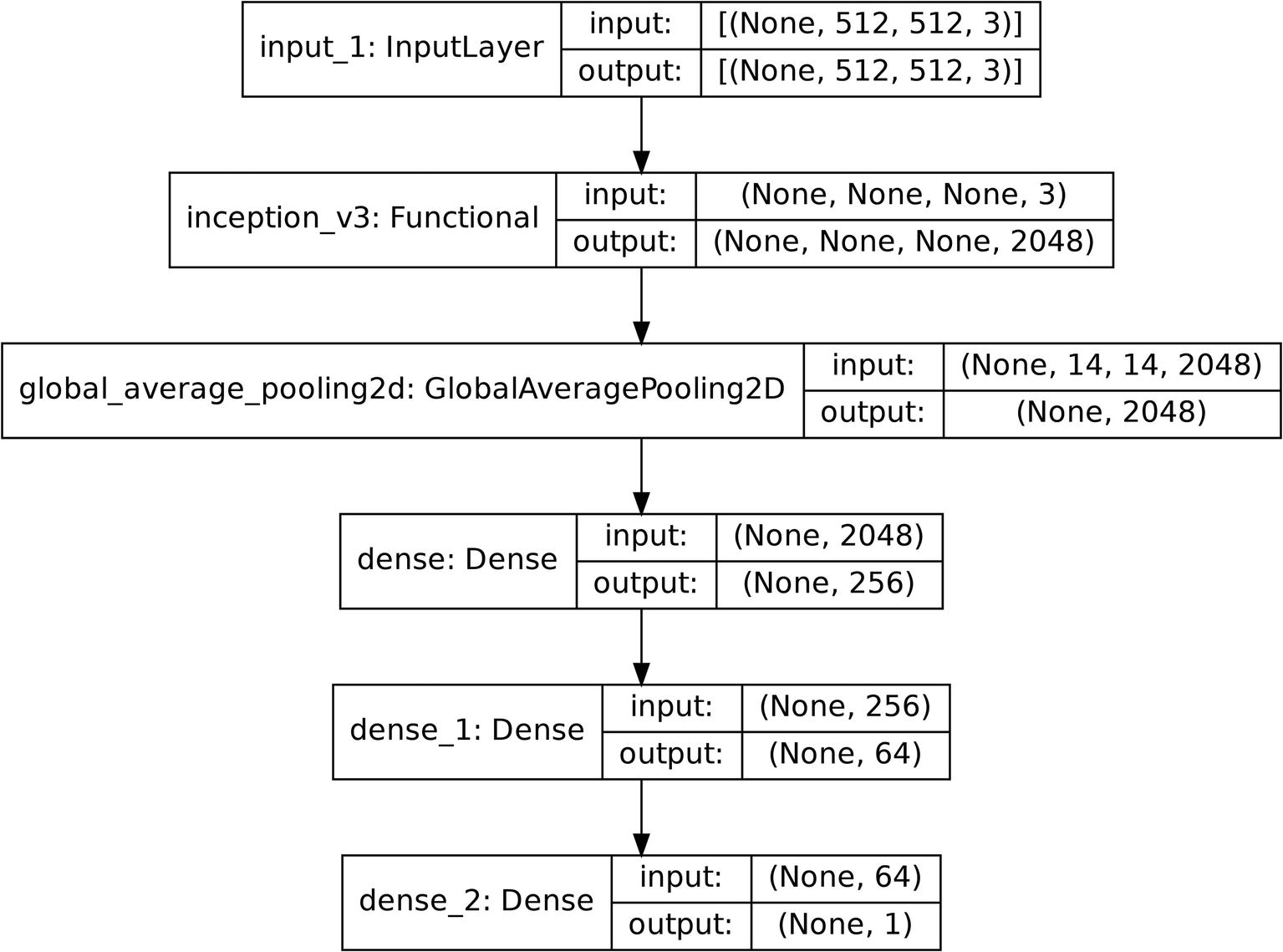
Diagram of an example model architecture using transfer learning
The model can be correspondingly compiled and trained. It should be noted that usually the fully connected component is much longer and complex to account for the complex nature of modern deep learning datasets.
Transfer Learning with Layer Freezing
In order to freeze a layer, set layer_obj.trainable=False.
Instantiating the pretrained model as a layer without directly taking in inputs
Compiling layers into a transfer learning model
Number of trainable and non-trainable parameters before layer freezing
Number of trainable and non-trainable parameters after layer freezing
Calling model.summary() is a good way to double-check if layer freezing worked or not. When several forms and series of neural network manipulations are being performed, it can be difficult to keep track and separate different forms of functions and instantiated objects.
You can unfreeze with inception_model.trainable = True and continue fitting again for fine-tuning.
You can also freeze individual layers with a similar method or by aggregating layers together into models and unfreezing groups of layers.
Accessing PyTorch Models
Keras/TensorFlow offers a large selection of pretrained models, and platforms like the model zoo (https://modelzoo.co/) or pypi libraries offer a wide range of pretrained models and/or architectures in Keras/TensorFlow.
PyTorch , a major alternative framework to Keras/TensorFlow, offers a larger selection of pretrained models. If a PyTorch pretrained model is not already implemented in Keras/TensorFlow, there’s a simple method to convert PyTorch models into Keras model objects so you can work with the model using familiar methods and steps.
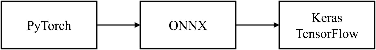
Diagram converting a PyTorch model to a Keras/TensorFlow model
Let’s start by installing PyTorch with pip install torch. It can be imported as import torch.
You can find a list of PyTorch image-based pretrained models at https://pytorch.org/vision/stable/models.html (note that you can access other non-image-based pretrained models as well). These image-based pretrained models can be accessed at torchvision.models.model_name. You can install TorchVision via pip with pip install torchvision.
Using PyTorch to instantiate a PyTorch pretrained model
Now that we have instantiated the PyTorch model, we can convert it into a Keras model using the pytorch2keras model, which can be installed via pip with pip install pytorch2keras.
Importing the necessary function to convert a PyTorch model to a Keras model
Converting a PyTorch model to a Keras model. Note that we did not explicitly import it, but np refers to numpy; this can be imported as import numpy as np
The input_np variable defines the shape of the input in channels-first format, where the “depth” of the image is listed as the first element of the shape. The torch.FloatTensor and torch.autograd.Variable functions convert the shape of the numpy array into valid tensor format.
The resulting Keras model can be visualized to double-check that the architecture has been transferred correctly and then compiled and fitted.
Note that not all PyTorch architectures can be converted into Keras/TensorFlow if some layer or operation is not supported for export by ONNX. See a list of transferable layers on the pytorch2keras GitHub: https://github.com/gmalivenko/pytorch2keras .
Implementing Simple Self-Supervised Learning
In this section, we will discuss the implementation of rudimentary level of self-supervised learning. You will find that many deep learning concepts are intertwined, and thus we need to wait until Chapter 3 because we first need to have a strong grasp of what autoencoders are before we understand their effective use in pretraining.
In more complex forms of self-supervised learning, modifications to the architecture are performed after the pretraining task often by adding more layers, usually to get the output into the desired shape to train on the task dataset or to add more processing power. In a simpler application of self-supervised learning, we will design our self-supervised pretraining strategy such that no architectural changes need to be made after pretraining and before formal training on the task dataset.
In order to design a self-supervised pretraining strategy that does not require any architecture changes, we need to focus primarily on the input and the output. If the shapes of the pretraining task’s x and y match that of the ultimate task’s, then there is no need to alter the architecture to accommodate it.
Consider the task of classifying the gender of a person in an image. Here, we have x = image and y = 1-dimensional vector (one value: 0 or 1, indicating gender). Thus, our self-supervised pretraining task should similarly require the model to take in an image and output one value.
For this example, the self-supervised pretraining task will be to identify the degree of noise. For each training example, we will add Gaussian noise with a certain standard deviation, σ. The objective of the model for pretraining is to predict the degree of noise, σ, given the noisy image. In order to perform such a task, the model would need to identify which features in the model count as noise and which ones do not, and thus it works toward discovering and representing fundamental structures and patterns in faces. Adding Gaussian noise changes the color of the images, not the “location” of certain features; since color determines the presence of shadows, edges, and other characteristics that define what a female and male face would generally look like, though, a good understanding of common relationships between the color of pixels between images would be valuable. Moreover, it moves the model closer toward being able to be robust to small perturbations and noise.
Fundamentally, at a rudimentary level without architecture changes, building self-supervised learning pretraining strategies is concerned primarily with data. We can build two datasets – augmented task dataset used for pretraining and a task dataset used for formal training – and fit the model on those two datasets, in that order. After being trained on the augmented task dataset, ideally the model will have developed representations of the “world” it is about to enter and can approach the ultimate task more aware and with more complex understandings than if it had not undergone pretraining.
To construct the augmented task dataset, we will use the .map method of loading images from directories into the efficient TensorFlow dataset format (see Chapter 1). For brevity, here we will provide only the function to be mapped in constructing the altered dataset.
Function to parse a file path using TensorFlow functions
TensorFlow function to implement an alteration to the dataset for pretraining
If you had a multidimensional output, you could also have the model predict changes to brightness, hue, etc. – features that are important to this task. TensorFlow offers a host of image processing and mathematical operations that you can use to alter data. It is best to stick to TensorFlow functions and objects when constructing functions to map to avoid errors or computational inefficiency.
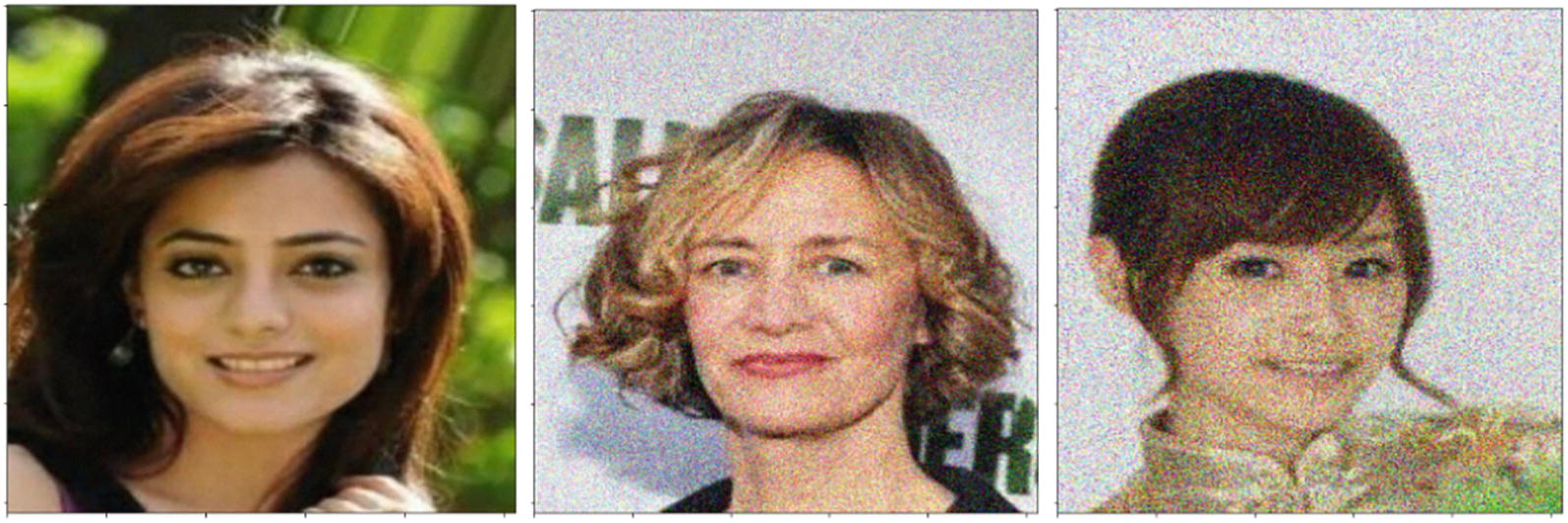
Example images from the altered task dataset. The standard deviations of noise (labels) for images from left to right are 0.003, 0.186, and 0.304
Performing pretraining and ultimate training
It should also be noted that the altered task dataset and the task dataset in this case are different types of problems – the former is a regression problem (predicting a continuous value), whereas the latter is a classification problem (categorizing an image). In this case, this difference is not a problem because all labels in both datasets reside between 0 and 1, meaning that a standard model with a sigmoid activation function output can operate on both. Binary cross-entropy is also a valid loss function for regression problems bounded between 0 and 1, although if you would like you can compile the model with a formally regression-based loss function (e.g., MSE, Huber) before training on the altered task dataset and recompile the model with binary cross-entropy (or some other loss function for classification) before training on the task dataset. In more advanced cases, adjusting from the altered task dataset to the task dataset requires making architectural modifications. You’ll find examples of this in the second case study of this chapter, as well as in Chapter 3 on autoencoders. With the tools of autoencoders, we can perform more complex pretraining strategies, like using image-to-image pretraining tasks (e.g., colorization, denoising, resolution recovery) to pretrain a model to perform an image-to-vector or image-to-image task.
Case Studies
These three case studies allow us to explore new ideas and recent research in transfer learning and self-supervised learning. Some ideas may be out of the scope of this book in terms of implementation but offer fresh perspectives and things to think about when designing your deep learning approaches.
Transfer Learning Case Study: Adversarial Exploitation of Transfer Learning
As deep learning models are increasingly deployed in common production, it is becoming more important to incorporate the findings from the rising field of adversarial learning into deep learning designs. Adversarial learning is concerned with how to exploit weaknesses in deep learning models, often by making small changes that are imperceptible to the human eye but that completely change the model’s output. Vulnerabilities in deep learning can lead to dangerous outcomes – imagine, for instance, if malicious or accidental alterations to a traffic sign cause a self-driving car to suddenly accelerate or brake.
In a 2020 paper entitled “A Target-Agnostic Attack on Deep Models: Exploiting Security Vulnerabilities of Transfer Learning,” Shahbaz Rezaei and Xin Liu6 explore how adversarial learning can be applied to transfer learning. Because many modern applications of deep learning use transfer learning, a malicious hacker could analyze the architecture and weights of the pretrained model to exploit weaknesses in the deployed model.
Rezaei and Liu show that a hacker, with knowledge only of the pretrained model used in the application model, can develop adversarial inputs leading to any desired outcome. Because the hacker does not need to know the weights or architecture of the application model or the data it was retrained on, the method of attack is target agonistic, which allows it to exploit wide swaths of deployed deep learning models that utilize publicly available pretrained models.
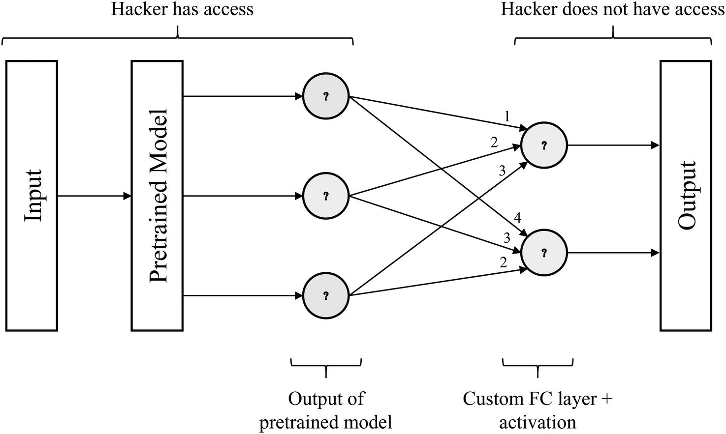
Example transfer learning model architecture with hacker visibility marked
The hacker has access only to the pretrained model, not the custom FC layer and any operations that process the output of the pretrained model.
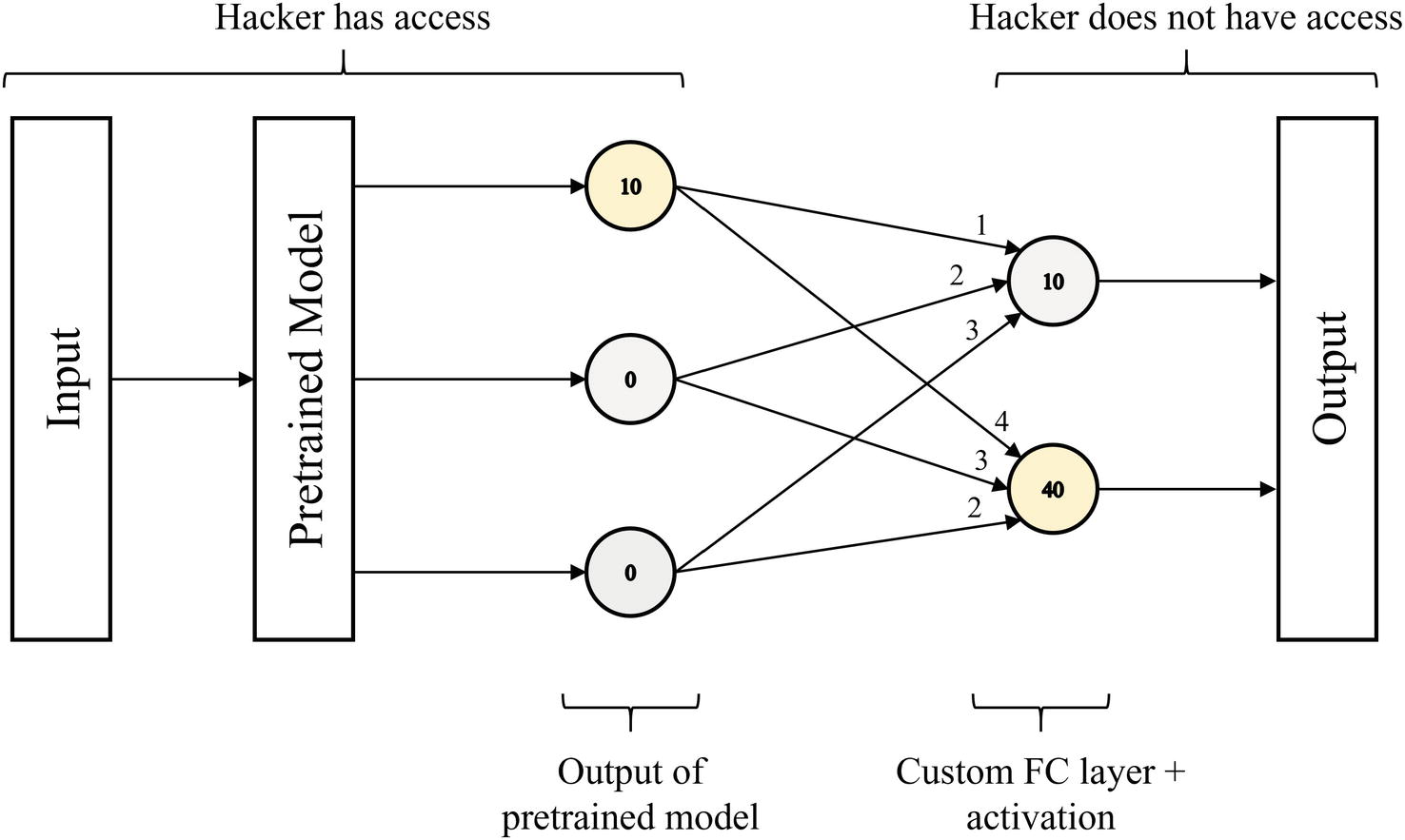
Example transfer learning model architecture with a pretrained model output neuron activated to trigger a specific output from the model
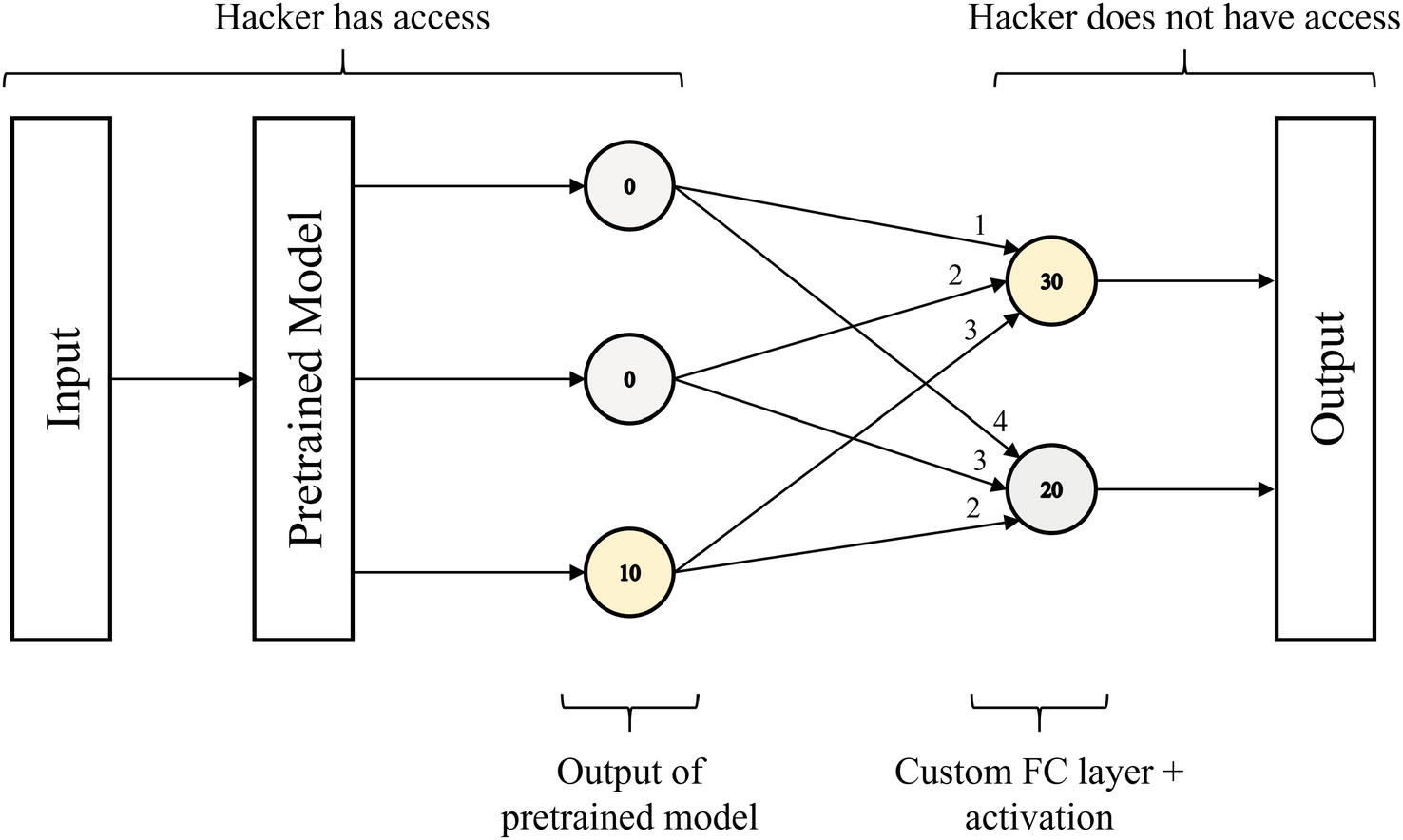
Example transfer learning model architecture with a pretrained model output neuron activated to trigger a specific output from the model
However, because the hacker does not know the weights outside of the pretrained model in the custom FC layer, they can perform a brute-force search to attempt to force the model to output a certain result. In this search, the hacker aims to construct an input such that the output of the pretrained model is [a, 0, …, 0, 0] the first time, [0, a, …, 0, 0] the second time, and so on until the last time, [0, 0, …, 0, a], where a is some arbitrarily large number. For each desired output, some node in the complete network’s output will be activated. The hacker simply records which one of the complete network’s output nodes is activated for each designed output of the pretrained model.
It should be noted that for this strategy to be capable of activating every output node of the complete model, for each output node of the complete model, there must exist a connection from an output node of the pretrained model whose weight is larger than the connection from the output node of that pretrained model to any other output node in the complete model. This may not be true in more complex datasets, especially heavy multiclass problems, but in most networks, this strategy works to “force” the network to predict almost any desired result.
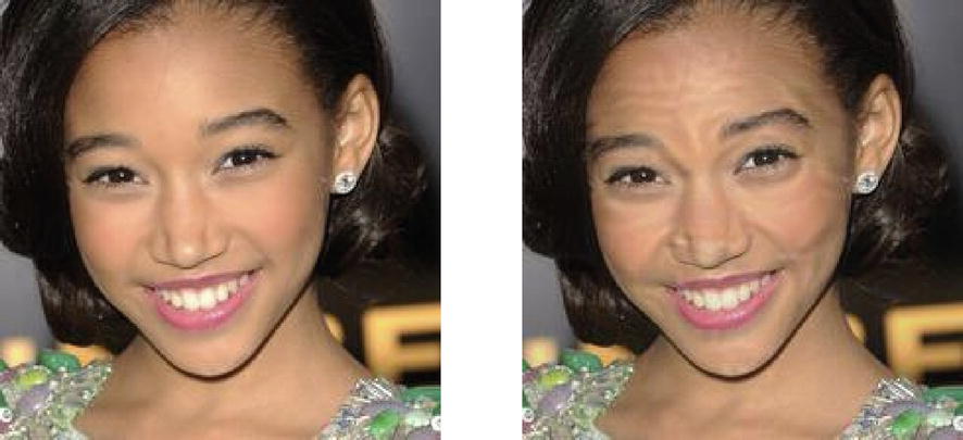
Left: example input image to the optimization algorithm. Right: example adversarial image generated to produce a certain network output. (By Shahbaz Rezaei and Xin Liu.)
Making small, specialized distortions to the original input image results in the model making different classifications between the first and second images. Moreover, this could be done without any knowledge of the complete networks’ weights or architectures – an impressive feat.
Metrics of attack performance for different numbers of target classes. Target classes: number of target classes/output nodes in the complete neural network. NABAC: number of attempts to break all classes, referring to the number of queries the attack needs to make to “break” a class (force the model to misclassify an item from that class as another class). Effectiveness (x%): the ratio of adversarial inputs that trigger a target class with x% confidence to the total number of adversarial inputs. (By Shahbaz Rezaei and Xin Liu.)
Target Classes | NABAC | Effectiveness (95%) | Effectiveness (99%) |
|---|---|---|---|
5 | 48.25 ± 42.5 | 91.68% ± 5.69 | 87.82% ± 6.98 |
10 | 149.97 ± 132.15 | 88.87% ± 2.46 | 83.07% ± 3.31 |
15 | 323.36 ± 253.56 | 87.79%± 2.42 | 82.08% ± 2.74 |
20 | 413 | 87.17% | 79.16% |
As the number of target classes increases, the attack needs to make more queries to break all classes, and its effectiveness decreases.
Metrics of attack performance for different numbers of layers. (By Shahbaz Rezaei and Xin Liu.)
# New Layers | NABAC | Effectiveness (95%) | Effectiveness (99%) |
|---|---|---|---|
1 | 48.25 ± 42.5 | 91.68% ± 5.69 | 87.82% ± 6.98 |
2 | 51.87 ± 39.94 | 91.57% ± 4.87 | 86.45% ± 5.35 |
3 | 257.26 ± 387.16 | 89% ± 8.20 | 85.67% ± 8.88 |
Nevertheless, the effectiveness is high, even as the number of target classes and new layers increases. This study is an interesting investigation into the implications of transfer learning for the deployment of models in real-world applications. It’s important to keep an eye toward deployment and the model’s role in the real world rather than in an airtight experimentation laboratory environment when designing deep learning approaches.
This overview was a simplification of the study; to read more, you can find the paper at https://openreview.net/pdf?id=BylVcTNtDS.
Self-Supervised Learning Case Study: Predicting Rotations
In “Unsupervised Representation Learning by Predicting Image Rotations,” Spyros Gidaris, Praveer Singh, and Nikos Komodakis7 propose a simple self-supervised learning method that develops strong representations of the data and yields effective results.
…it is essentially impossible for a ConvNet model to effectively perform the above rotation recognition task unless it has first learnt to recognize and detect classes of objects as well as their semantic parts in images. More specifically, to successfully predict the rotation of an image the ConvNet model must necessarily learn to localize salient objects in the image, recognize their orientation and object type, and then relate the object orientation with the dominant orientation that each type of object tends to be depicted within the available images.
—Gidaris et al., “Unsupervised Representation Learning by Predicting Image Rotations”
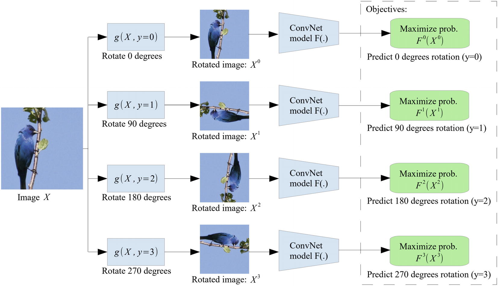
The convolutional neural network’s prediction objectives under self-supervised learning by predicting rotations. (By Gidaris et al.)
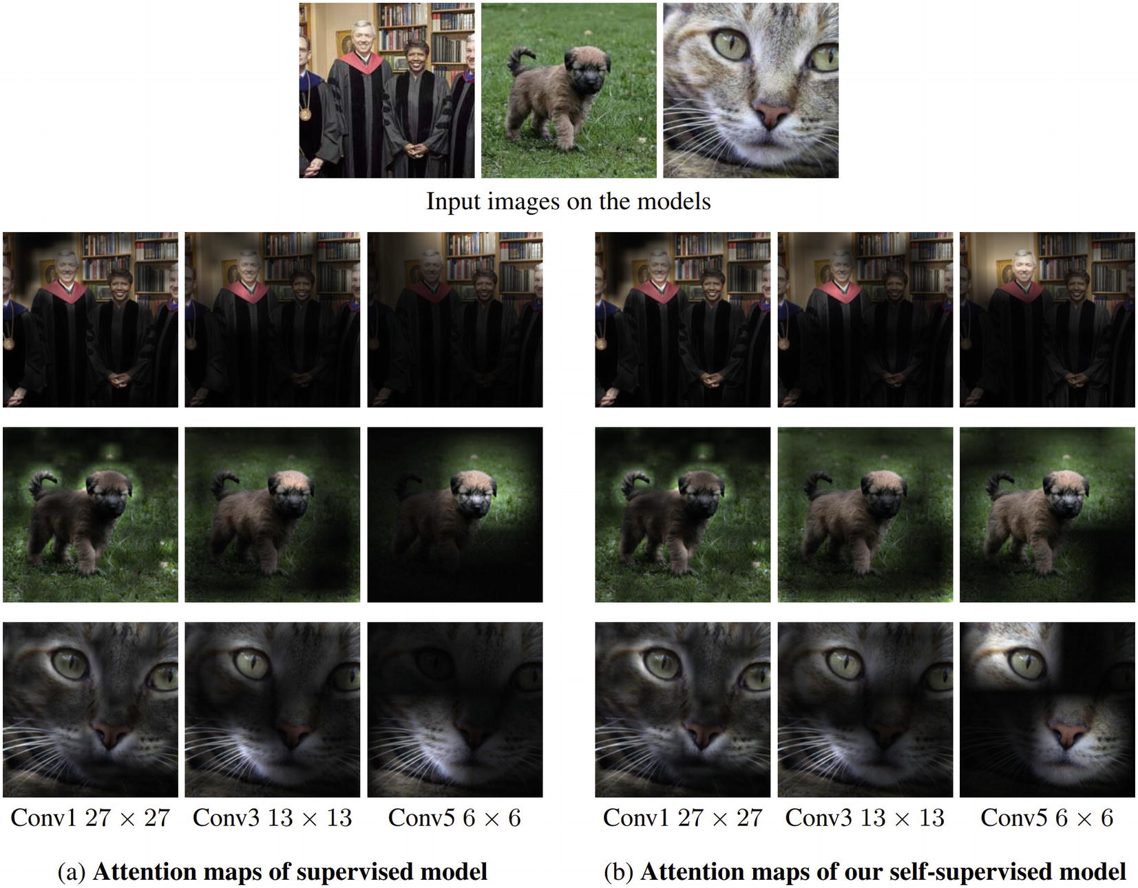
Attention maps from various layers from a supervised model and a self-supervised model given three example input images. (By Gidaris et al.)
The attention map of a convolutional layer can be found by computing the feature maps for that layer and aggregating them. You can visually see that the attention maps from the self-supervised model focus more on the high-level objects, like the eyes, nose, tails, and heads – in accordance with important features required to perform object recognition.
You can perform something similar by extracting features from a layer in the middle of a neural network in Keras by referring to individual layers (assuming each layer is associated with a variable you defined using the Functional API). Visualizing layer weights and features can be helpful to understanding the improvement in representation capabilities that self-supervised learning provides.
Performance on CIFAR-10 classification for different rotations needed for prediction. (By Gidaris et al.)
# Rotations | Rotations | CIFAR-10 Classification Accuracy |
|---|---|---|
8 | 0°-45°-90°-135°-180°-225°-270°-315° | 88.51 |
4 | 0°-90°-180°-270° | 89.06 |
2 | 0°-180° | 87.46 |
2 | 90°-270° | 85.52 |
Constructing rotation-based altered task dataset
We’ll use the EfficientNetB4 architecture (not using its weights) to predict which one of four rotations was applied (Listing 2-21). Note that the output of the EfficientNetB4 architecture is 100-dimensional, which is projected via the final layer out into the four desired outputs. A more efficient approach, at first glance, may seem to simply define the number of output classes in the base EfficientNetB4 model to be 4. We will see soon why this design instead is required for this sort of self-supervised learning operation.
Constructing model architecture
Constructing model architecture
After fitting on the altered task dataset, though, we run into a problem: the current model outputs only four values, since the altered task dataset had four unique labels, but the task dataset (i.e., the formal CIFAR-10) dataset has ten classes. This requires an architectural modification.
Constructing model architecture
If we instead had trained a base model with output four classes and attached another output layer with ten classes afterward, which is another technically available option (in that the code runs), performance would likely be poor due to the bottleneck imposed by the four-class output. In this case, think of the EfficientNet model not as outputting 100 classes but as outputting 100 features that are compiled and used to make decisions in the output layer. The base model still contains all the weights learned from self-supervised learning. The new model can then be compiled and trained on the task dataset.
This self-supervised learning approach drastically improves the state-of-the-art results on unsupervised feature learning for a variety of object detection tasks, including ImageNet, PASCAL, and CIFAR-10.
The work of Gidaris et al. points to the existence of simple yet effective approaches to apply self-supervised learning to boost deep learning model performance.
Self-Supervised Learning Case Study: Learning Image Context and Designing Nontrivial Pretraining Tasks
Earlier , we discussed relatively simpler self-supervised learning examples, like adding noise to the task dataset and pretraining the model to predict the degree of noise. Other examples were simple conceptually (although perhaps difficult to implement or accomplish), like pretraining the model to colorize grayscale images. While sometimes simpler self-supervised strategies like predicting the degree of rotation are effective, in other occasions for a bigger performance boost, a more complex pretraining task needs to be used.
Carl Doersch, Abhinav Gupta, and Alexei A. Efros propose a complex, creative, and effective self-supervised learning pretraining task in their 2016 paper, “Unsupervised Visual Representation Learning by Context Prediction.”8 Their design is a great case study of the implications and possibilities that need to be considered to design a successful self-supervised pretraining strategy.
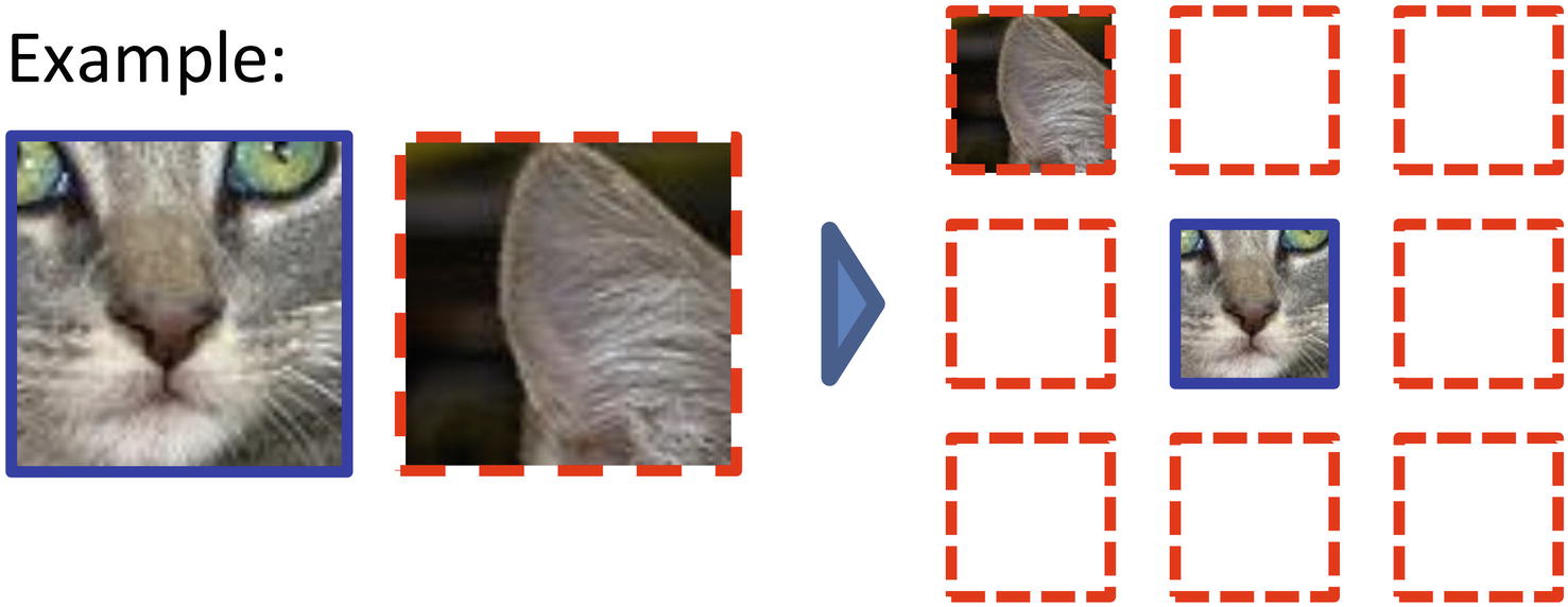
Example context and patch relationships
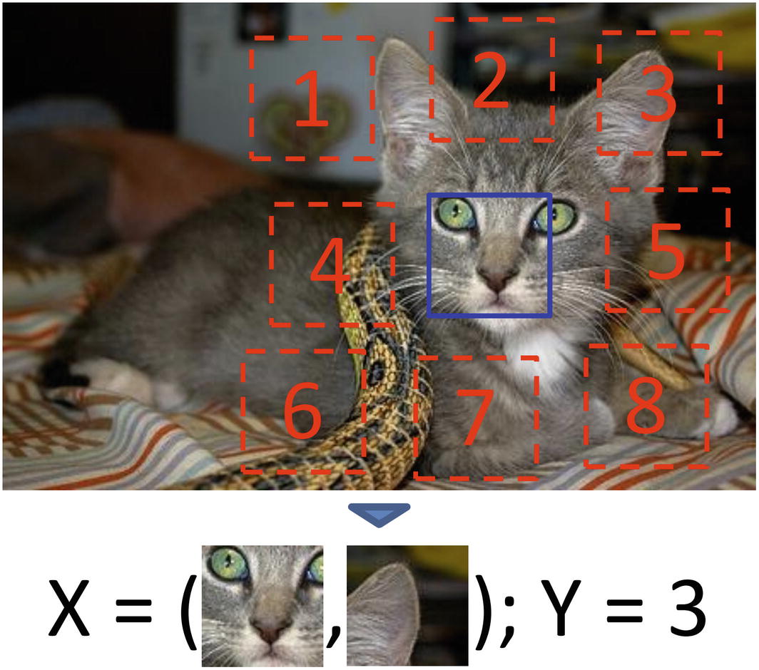
Assigning numbers to neighbor patch directions
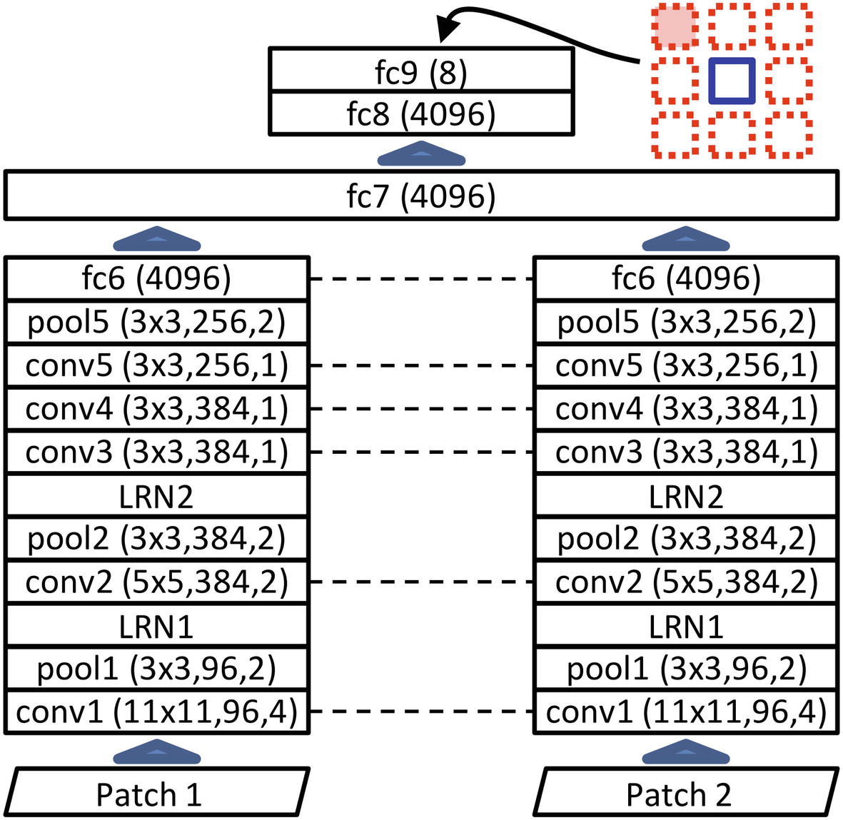
Two-input architecture used to perform the pretraining task
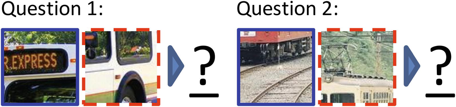
Example “questions” with two patch pairs of inputs
However, Doersch et al. found that the neural network was learning “trivial solutions” – that is, it was finding shortcuts and easy approaches to the pretraining task that were not related to the concepts Doersch et al. had hoped it would learn.
For instance, low-level cues like boundary patterns or the continuation of textures across patches serve as trivial shortcuts that the neural network can exploit without learning the high-level relationships it would ideally learn. To address this, Doersch et al. added both a gap between patches about half the length of the patch width and a random “jitter” for each patch location by up to 7 pixels. (These are shown visually in Figure 2-32.) With these modifications, the network could not reliably exploit trivial shortcuts like the continuation of textures and lines.
However, another unexpected problem arose: a phenomenon called chromatic aberration, in which light rays pass through a lens focus at different points depending on their wavelength. Thus, in camera lenses that are affected by chromatic aberration, one color – usually green – is “shrunk” toward the center of the image relative to other color channels (red and blue). The network can thus parse the absolute location of patches by detecting the shape and position of the separation between green and magenta (the color comprising the non-green color channels, red and blue). Finding the relative position given knowledge about the absolute location of two patches thus becomes a trivial task.
To address this, Doersch et al. randomly dropped two of three color channels from each patch and replaced the dropped channels with Gaussian noise. This method prevents the neural network from exploiting information in the color channels and instead to focus on the general shapes and edges – the higher-level features – in its pretraining task.
By making modifications to the architecture, like only using one “branch” and adding more convolutional layers, Doersch et al. converted the two-image-to-vector architecture into an image-to-vector architecture. The authors tested this pretrained architecture on the PASCAL Visual Object Classes (VOC) Challenge and found that this self-supervised learning strategy was the best result without using labels not included in the dataset (to their knowledge, and at the time of paper release). The authors found in other datasets that this context prediction task yielded a significant boost to model performance.
This paper is both an example of a well-thought-out self-supervised learning pretraining task and of the process of modifying the pretraining task to accomplish the ultimate objective by discouraging trivial solutions. Self-supervised learning offers us a clever way to find, extract, and utilize rich insights and information without needing to search for costly labels and wandering outside of the dataset.
Key Points
Pretraining is a task that is performed before the formal training of a model and can orient the model toward better performing on its ultimate task.
Because pretraining moves the model into a more convenient location in the loss landscape, it can arrive at a better solution more quickly than a model without pretraining. Thus, pretraining generally has two key advantages that boost model performance: decreased time and better metric scores.
- Transfer learning uses two separate datasets – a general dataset and a task dataset. The model is first trained on the general dataset, and then the learned weights and “skills” from the task are transferred to another model that is trained on the task dataset. Pretrained models are often kept in publicly available repositories and can be accessed and used in your own model.
Image-based pretrained models generally consist of two components: a feature extraction component and a fully connected component (the “top”). You can (a) keep only the feature extraction component and build a custom FC component, (b) keep both the feature extraction component and the fully connected component only, or (c) keep both the feature extraction component and the FC component, but add more layers afterward.
Layer freezing allows you to selectively train certain parts of a model using transfer learning to better take advantage of pretrained weights. Usually, weights from the pretrained model are frozen and the custom added layers are trained. After this step, sometimes the pretrained model is unfrozen and the entire network is trained to fine-tune on the data.
Keras/TensorFlow has built in a repository of pretrained models organized into modules, in which each module contains the pretrained model(s) and associated functions (usually for encoding and decoding). Important pretrained models include the ResNet family, the InceptionV3 model, the MobileNet family, and the EfficientNet family. Keras/TensorFlow models are pretrained on the ImageNet dataset. You can also convert PyTorch models into Keras/TensorFlow models to take advantage of PyTorch’s large repository of pretrained models.
- Self-supervised learning uses pretrains on an altered task dataset derived from input data of the task dataset. The x and y of the altered task dataset come completely from only the x of the task dataset, often by performing distortions or actions to generate labels. Self-supervised learning helps orient the model to representing and understanding the “world” of the dataset so it is prepared to understand the dynamics and core features of the task dataset.
Self-supervised learning is especially valuable for training on small datasets with few labels, or when there is an abundance of unlabeled data that otherwise would not have been used.
There are two key differences between transfer learning and self-supervised learning. Firstly, the pretraining dataset and the task dataset generally come from completely different sources in transfer learning, whereas in self-supervised learning, the pretraining dataset is derived from the input data of the task dataset. Secondly, transfer learning aims to develop “skills,” while self-supervised learning encourages “representations of the world.”
Although we implemented relatively simple models and methods in this chapter, with these conceptual tools and the design intuition of what transfer learning and self-supervised learning are, you will be able to build many more complex training structures, like stacking pretrained models (“double transfer learning”) or designing innovative self-supervised pretraining methods.
In the next chapter, we’ll expand upon our study of advanced neural network structures and manipulations with autoencoders, a versatile tool often used in developing successful training structures.