One word is worth a thousand pictures, if it’s the right word.
—Edward Abbey, American author and essayist1
The concept of encoding and decoding entities – ideas, images, physical material, information, and so on – is a particularly profound and important one, because it is so deeply embedded into how we experience and understand the environment around us. Encoding and decoding information is a key process in communication and learning. Every time you communicate with someone, observe the weather, read from a book – like this one – or in some way interact with information, you are engaging in a process of encoding and decoding, observing and interpreting. We can make use of this idea with the deep learning concept of an autoencoder.
This chapter will begin by exploring the intuition and theory behind autoencoders and how they can be used. It will also cover Keras neural network manipulation methods and neural network design that are integral to implementing not only autoencoders but also other more complex neural network designs in later chapters. The other major half of the chapter will be dedicated toward exploring the versatility of autoencoders through five applications. While the autoencoder is a simple concept, its incorporation into efforts tackling deep learning problems can make the difference between a mediocre and a successful solution.
Autoencoder Intuition and Theory
Although we will clarify what encoding and decoding refer to more specifically with relevance to the intuition behind autoencoders, for now they can be thought of as abstract operations tied inextricably together to one another. To encode an object, for our purposes, is to represent it at a loss of quantifiable information. For instance, we could encode a book by summarizing it, or encode an experience with key sensory aspects, like notable senses of touch or hearing. To decode is to take in the encoded representation of the object and to reconstruct the object. It is the objective of encoding and decoding to “work together” such that the reconstruction is as accurate as possible. An effective summary (encoding) of a book, for instance, is one from which a reader could more or less construct the main ideas of the book to a high accuracy.
Suppose someone shows you an image of a dog. They allow you to look at that image for a few seconds, take it away, and ask you to reconstruct the image by drawing it. Within those few seconds, ideally you would have extracted the key features of that image so that you could draw it as accurately as possible through some efficient method. Perhaps you remember that the dog was facing right, its head upright, that it was tall, and that it looked like it was standing still.
What is interesting is that these are all high-level abstract concepts – to deduce that an object is facing a certain direction, for instance, you must know the relationship between the directions of each of the object’s parts (for instance, if the head is facing one way, the tail should be facing the other) and be able to represent them in a spatial environment. Alternatively, knowing that a dog is tall requires knowledge of what a “standard” or “short” dog looks like. Identifying the absence of motion requires knowledge of what motion for this particular class of objects looks like.
The key idea here is that for effective compression and reconstruction of an object in the context of complex objects and relationships, the object must be compressed with respect to other objects. Compressing an object in isolation with a high reconstruction performance is more difficult or performs worse than compressing an object with access to additional sets of related knowledge. This is why recovering an image of a dog is easier than recovering an image of an unfamiliar object. With the image of the dog, you first identify that the object is a dog and thus identify that knowledge relating to the “dog” entity is relevant and then can observe how the image deviates from the template of the dog. When decoding, if you already know that the image was of a dog (a technical detail: this information can be passed through the encoding), you can do most of the heavy lifting by first initializing the knowledge related to a dog – its standard anatomy, its behavior, and its character. Then, you can add deviations and specifics, as necessary.
Because efficient compression of complex entities requires the construction of highly effective representations of knowledge and of quick retrieval, this encoding-decoding pair of operations is extremely useful in deep learning. This pair of operations is referred to generally as the autoencoder structure, although we will explore more solidly what it entails. Because the processes of encoding and decoding are so fundamental to learning and conducive to the development of effective representations of knowledge, autoencoders have found many applications in deep learning.
Likewise, it should be said that this sort of dependence on context makes autoencoders often a bad approach for tasks like image compression that require a more universal method of information extraction. Autoencoders are limited as tools of data compression to the context of the data they are working with and even with that context perform at best equivalently to existing, more universal compression algorithms. For instance, you could only train a standard autoencoder to effectively encode a few pineapple images if you fed it thousands of other images of pineapples; the autoencoder would fail to reconstruct an image of an X-ray, for instance. This is a good example of critically evaluating deep learning’s viability as an approach to certain problems and a much needed reminder that deep learning is not a universal solution and needs to work with other components to produce a complete product.
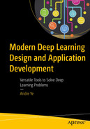
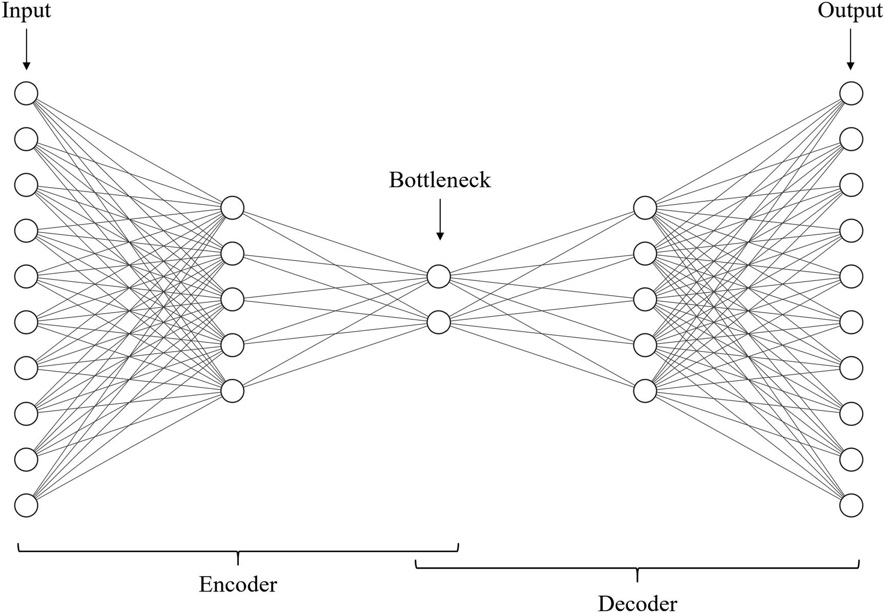
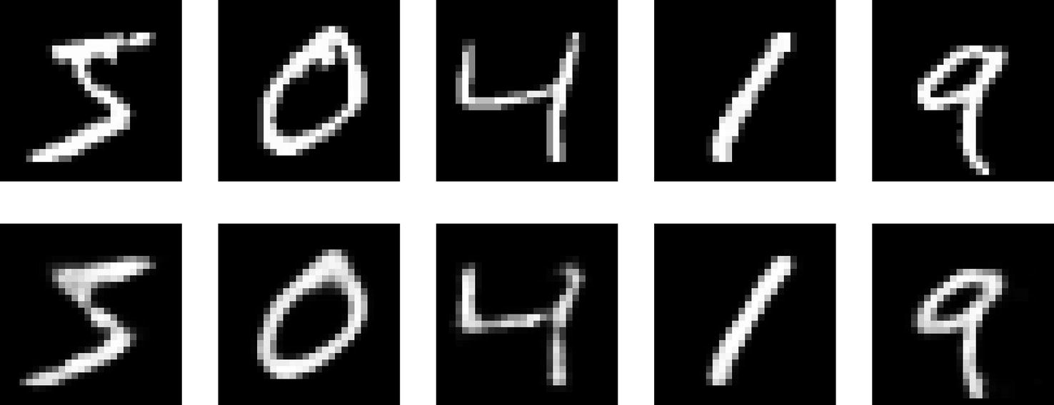
Top row: inputs/original images. Bottom row: reconstructed inputs
Despite the autoencoder being an unsupervised task – there are no labels – it is able to perform highly effective clustering and learn key features, attributes, and structures of the data.
Components of an autoencoder diagram
The input and output of autoencoders have the same size, because autoencoders are trained on the task of reconstruction – given an input item, the objective is to reconstruct the output with as high accuracy as possible. This is a crucial feature of autoencoders that will be core to how we go about designing these structures.
Original images and their reconstructions by an autoencoder with a small bottleneck size
Original images and their reconstructions by an autoencoder with a large bottleneck size
Most of the “meat” within autoencoder usage resides in their applications. We’ll begin by discussing how autoencoders are designed and implemented for tabular data and image data. Then, we’ll explore the intuition and implementation for five applications of autoencoders.
The Design of Autoencoder Implementation
There are many considerations to be made in the implementation of autoencoders, depending on the form of their application. In this section, we will broadly discuss considerations for designing autoencoders on one-dimensional (vector) and two-dimensional (tabular) data by example.
Autoencoders for Tabular Data
Tabular data , for our purposes, refers to data that can be put in the form (n, s), where n indicates the number of data points and s indicates the number of elements in each data point. The entire dataset can be put into a two-dimensional table, where each row indicates a specific data point and each column indicates a feature of that data point.
Building autoencoders for tabular data is an appropriate place to begin, because the shape of data at any one layer can be easily manipulated simply by changing the number of nodes at that layer. The shape of other forms of data, like images, is more difficult to handle. Being able to manipulate shape is crucial to autoencoder design because the concept of encoding and decoding entities comes with relatively strict instructions about what the shape of the data should look like before encoding, after encoding, and before decoding.
The difference between a standard autoencoder (often abbreviated simply as “AE”) and a “deep autoencoder” should also be noted here. Although the exact terminology has not seemed to have stabilized yet, generally an autoencoder refers to a shallow autoencoder structure, whereas a deep autoencoder contains more depth. Often, this is determined by the complexity of the input data, since more complex forms of data usually necessitate greater depth. Because data that can be arranged in a tabular format is generally less complex than image or text data (or other sorts of highly specialized and complex data that neural networks have become good at modeling), it’s generally safe to refer to autoencoder structures used on high-resolution sets of images or text as deep autoencoders and autoencoder structures used on tabular data as simply autoencoders.
Importing important layers and models
Once we initialize the Sequential model structure, we can add the Input layer, which takes in the 784-dimensional input data.
Building a simple encoder using Dense layers for tabular data
The last layer of the encoder contains 32 nodes, indicating that the bottleneck will be 32 nodes wide. This means that, at its most extreme, the autoencoder must find a representation of 784 features with 32 values.
It should also be noted that it is convention for the number of nodes in each layer to be a power of two. You will see this pattern both throughout examples in this book and in the architectures of neural networks designed by researchers (some of these are presented in case studies). It’s thought by many to be convenient for memory and a good way to scale the number of nodes meaningfully (when the number of nodes is high, meaningful change is proportional rather than additive). This convention by no means is required, though, if your design requires node quantities that cannot accommodate this convention.
Building a simple decoder using Dense layers for tabular data
Note that, in this example, the activation for the last layer of the model is the sigmoid activation function. We traditionally put the sigmoid activation (or other related curved and bounded functions and adaptations) on the last layer to bound the neural network for classification problems. This may or may not be suitable toward your particular task.
If your input data consists of entirely binary data or can be put into that form appropriately, sigmoid may be an appropriate activation. It is important to make sure that your input data is scaled properly; for instance, if a feature is binary in that it contains only the values 10 and 20, you would need to adjust the feature such that it consists only of the values 0 and 1. Alternatively, if your feature is not strictly binary but tends to cluster around two bounds, sigmoid may also be an appropriate choice.
On the other hand, if a feature is spread relatively uniformly across a wide range, it may not be appropriate to use the sigmoid activation. The sigmoid function is sloped such that it is more “tricky” to output an intermediate value near 0.5 than near 0 or 1; if this does not adequately represent the distribution of a feature, there are other options available. An activation like ReLU (Rectified Linear Unit, defined as y = max(x, 0)) may be more appropriate. However, if your feature ranges across negative outputs as well, use the linear activation (simply y = x). Note that depending on the character of the features in tabular data, you will need to choose different losses and metrics – the primary consideration being regression or classification.
A challenge of autoencoders for tabular data is that often tabular data is not held together by a unifying factor of context in the same way that image or text is. One feature may be derived from a completely different context than another feature, and thus you may simultaneously have a continuous feature and a categorical feature that a tabular autoencoder must both accommodate. Here, feature engineering (e.g., encoding categorical features to continuous values) is needed to “unify” the problem types of the features.
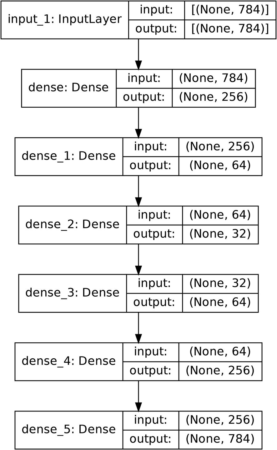
Sample autoencoder using only Dense layers for tabular data
When building autoencoders, however, generally a compartmentalized design is preferred over sequentially stacking layers. A compartmentalized design refers to implementing a model as a relationship between several sub-models. By using a compartmentalized design, we can easily access and manipulate the sub-models. Moreover, it is more clear how the model functions and what its components are. In an autoencoder, the two sub-models are the encoder and the decoder.
To build with a compartmentalized design, first define the architectures of each of the sub-models. Then, use the Functional API to define each sub-model as an input of another object and aggregate the sub-models into an overarching model using keras.models.Model.
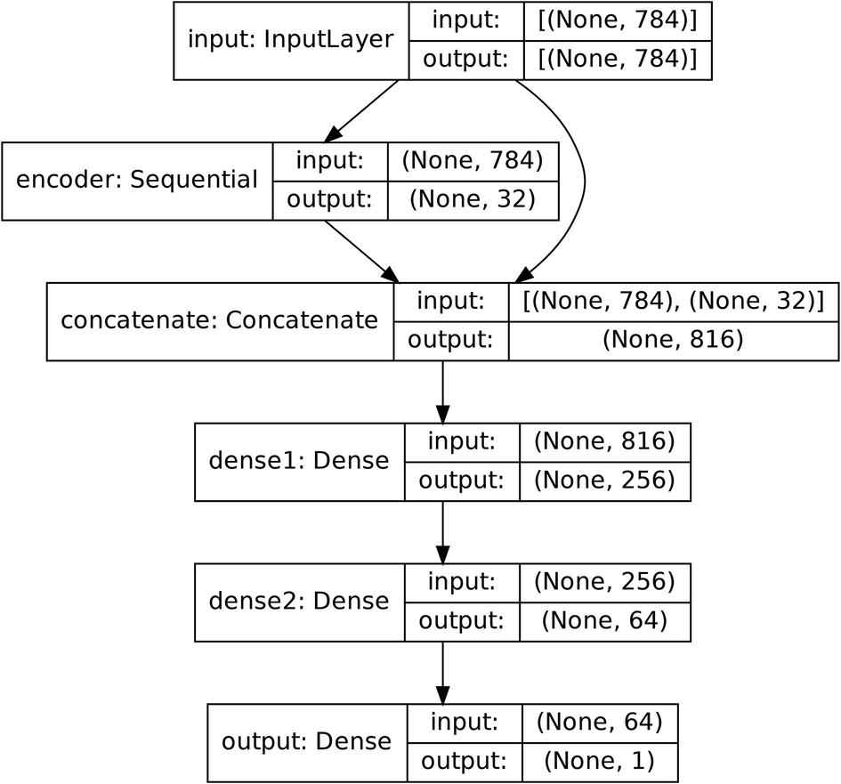
Building a simple encoder and decoder using Dense layers for tabular data with compartmentalized design
Compiling sub-models into an overarching model – the autoencoder – with compartmentalized design and the Functional API

Visualization of an autoencoder architecture built with compartmentalized design
The primary practical benefit of using compartmentalized design for autoencoders is that after compiling and fitting, we can call encoder.predict(input_data) to obtain the learned encoding. If you do not use compartmentalized design, you can also use layer-retrieving methods discussed in Chapter 2 (e.g., get_layer()) to create a model object consisting of the encoding layers, but it’s more work than is necessary and is less portable. Accessing the encoder’s encoding of data is necessary for many of the autoencoder applications we will discuss in the second half of this chapter.
As mentioned in Chapter 2, you can use this implementation design method with all sorts of other structures beyond autoencoders to easily freeze entire groups of layers, or for the other benefits of compartmentalized design mentioned here, like better organization or easier referencing of models. For instance, this sort of compartmentalized design can be used to separate a model using transfer learning into two sub-models: the pretrained convolutional component and the custom fully connected layer. Freezing the pretrained convolutional component can be easily done by calling submodel.trainable = False.
Autoencoders for Image Data
Building autoencoders for image data follows the same logic as building one for tabular data: the encoder should condense the input into an encoded representation by using “reducing” operations, and the decoder should expand the encoded representation into the output by using “enlarging” operations. However, we need to make additional considerations to adapt to an increased complexity of the data shape.
The “enlarging” operation needs to be some sort of an “inverse” of the “reducing” operation. This was not much of a concern with Dense layers, because both an enlarging and a reducing operation could be performed simply by increasing or decreasing the number of nodes in a following layer. However, because common image-based layers like the convolutional layer and the pooling layer can only be reductive operations, we need to explicitly note that the decoding component is not only the encoding component “in reverse” (as was described in building autoencoders for tabular data) but is inverting – step by step – the encoding operations. This poses complications to building the encoder and decoder.
Although there are developments on using deep autoencoders for language and advanced tabular data, autoencoders have primarily been used for image data. Because of this, an extensive knowledge of autoencoders is necessary to successfully deal with most image-related deep learning tasks.
Image Data Shape Structure and Transformations
Because shape is so important to convolutional autoencoder design, first, we must briefly discuss image shape and methods of transforming it.
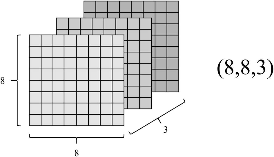
Illustration of the three dimensions of an image
Important layers in a convolutional neural network and their transformations to the image shape
Layer | Parameters | Output given input shape (a, a, c) | Description |
|---|---|---|---|
Convolution | Kernel shape = (x, y) Number of filters = n Padding = “same” or “valid” | If padding = 'valid': (a-(x-1), a-(x-1), n) If padding = 'same': (a, a, n) | The two-dimensional convolution slides a kernel of shape (x, y) across the image. Hence, it will reduce the image’s spatial dimensions by x-1 and y-1 pixels. Generally x=y (thus the kernel is square-shaped), but some architectures exploit a rectangular kernel shape, which can be successful in certain domains. See the Chapter 6 case study on the InceptionV3 architecture to explore convolution factorization and nonsquare kernel shapes. However, if padding is set as “same,” the image is padded (extra “blank” dimensions are added to its size) such that when the convolution is performed, the resulting image has the same shape as the previous one. We’ll see why this is helpful later. |
Pooling | Pooling size = (x, x) Padding = “same” or “valid” | If a is divisible by x and padding='same' or 'valid': (a/x, a/x, c) If a is not divisible by x and padding='valid': (floor(a/x), floor(a/x), c) If a is not divisible by x and padding='same': (ceil(a/x), ceil(a/x), c)2 | The two-dimensional pooling operation offers a faster way to reduce the size of an image shape by placing non-overlapping (unlike convolutions, which do overlap) windows of size (x, x) across the image to “summarize” the important findings. Pooling is usually either used in the form of average pooling (all elements in the pooling window are averaged) or max pooling (the maximum element in the pooling window is passed on). Pooling divides the image size by the pooling window’s respective dimension. However, because images sometimes may not be exact multiples of the window’s respective dimension, you can use padding modes to help determine the exact shape of the output. |
Transpose convolution | Kernel shape = (x, y) Number of filters = n Padding = “same” or “valid” | If padding = 'valid': (a+(x-1), a+(x-1), n) If padding = 'same': (a, a, n) | The transpose convolution can be thought of as the “inverse” of the convolution. If you passed an input through a convolutional layer and then a transpose convolutional layer (with the same kernel shape), you’d end up with the same shape. When you’re building the decoder, use transpose convolutional layers in lieu of the convolutional layers in the encoder to increase the size of the image shape. Like the convolutional layer, you can also choose padding modes. |
Upsampling | Upsampling factor: (x, y) | (a*x, a*y, n) | The upsampling layer simply “magnifies” an image by a certain factor without changing any of the image actual values. For instance, the array [[1, 2], [3, 4]] would get upsampled simply as [[1, 1, 2, 2], [1, 1, 2, 2, ], [3, 3, 4, 4], [3, 3, 4, 4]] with an upsampling factor of (2,2). The upsampling layer can be thought of as the inverse of the pooling operation – while pooling divides the dimensions in the image size by a certain quantity (assuming no padding is being used), upsampling multiples the image size by that quantity. You cannot use padding with upsampling. When you’re building the decoder, use upsampling layers in lieu of pooling layers in the encoder to increase the size of the image shape. |
Note that only convolutional and transpose convolutional layers contain weights; pooling and upsampling are simple ways to aggregate extracted features without any particular learnable parameters. Additionally, note that the default padding method is “valid.”
There are many approaches to building convolutional autoencoders. We’ll cover many approaches, beginning with a simple convolutional autoencoder without pooling to introduce the concept.
Convolutional Autoencoder Without Pooling
As noted before, autoencoders are generally built symmetrically, but this is even more true with image-based autoencoders. In this context, not building the autoencoder symmetrically requires a lot of arduous shape tracking and manipulation.
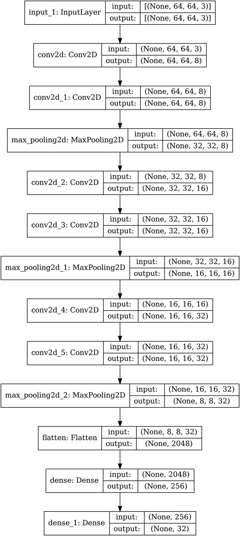
Building an encoder for image data using convolutions without pooling
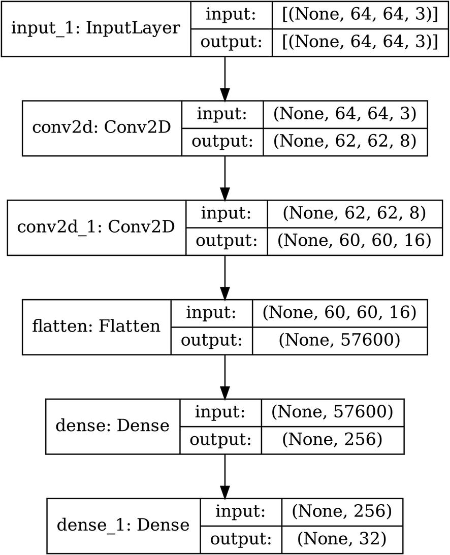
In this case, we are successively increasing the number of filters (from 3 channels initially to 8, 16, and 32) while keeping the filter size at (3,3).
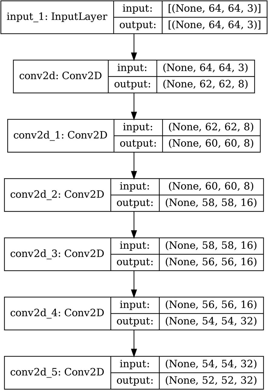
The architecture of an example convolutional encoder without pooling and only using convolutional layers
Building a decoder for image data using convolutions without pooling
The architecture of an example convolutional decoder without pooling and only using convolutional layers
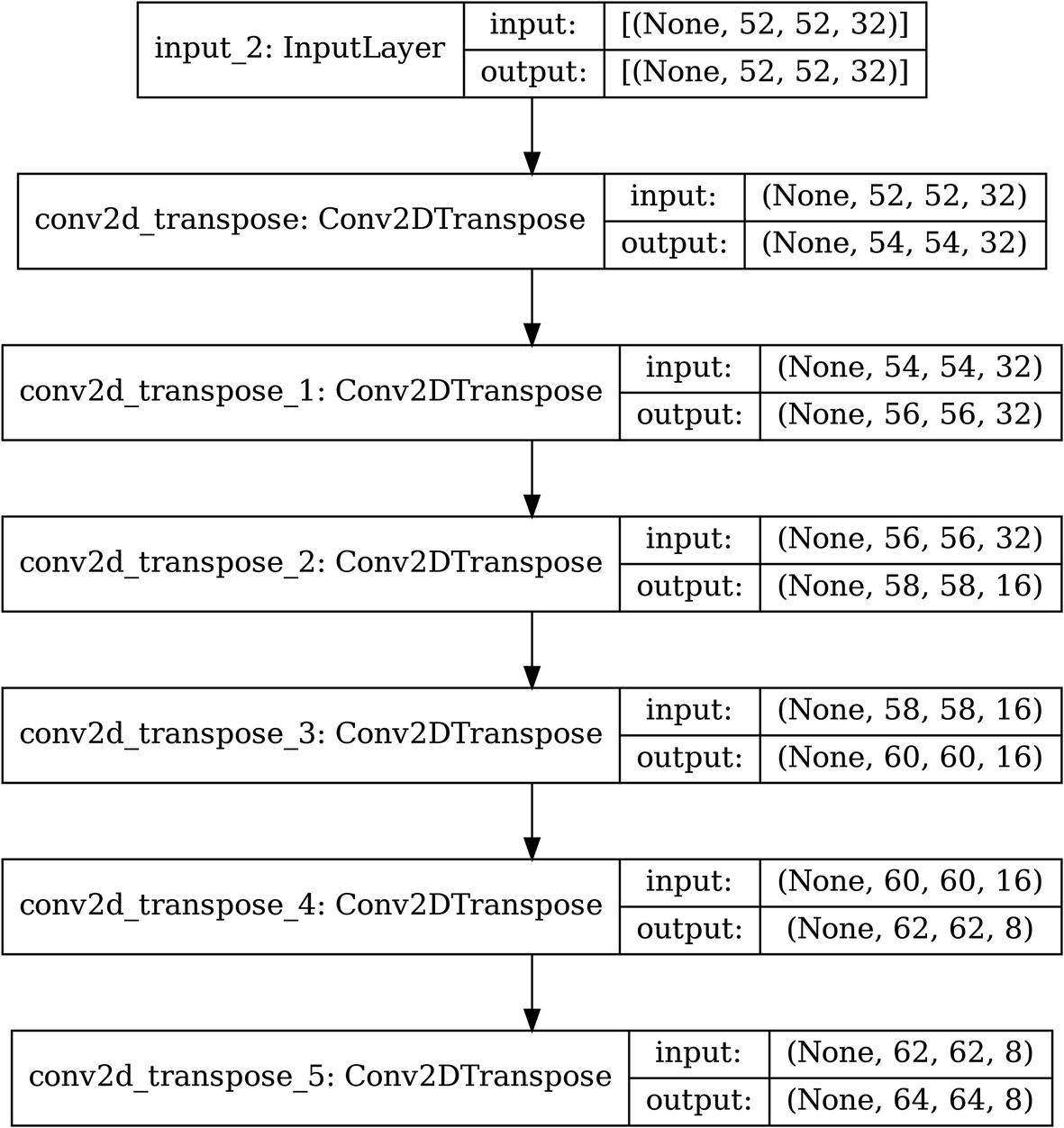
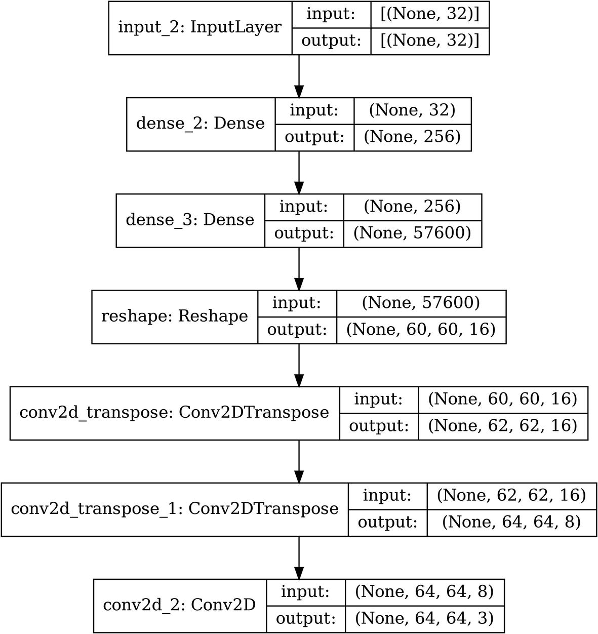
There’s one problem – the output of the decoder has shape (64, 64, 8), whereas the input has shape (64, 64, 3). There are two ways of addressing this. You could change the last layer to L.Conv2DTranspose(3, (3, 3)) such that it has three channels. Alternatively, you could add another layer to the end of the decoder: L.Conv2DTranspose(3, (1, 1)). Because it has a filter size of (1,1), the image width and height are not changed, but the number of channels is collapsed from 8 into 3.
Building long, repeated architectures using for loops and lists of parameters accordingly referenced within the loop
Building long, repeated architectures using for loops without lists of parameters accordingly referenced within the loop
A primary benefit of this sort of design is that you can easily extend the depth of the network simply by increasing the number of iterations layer-adding code is looped through, saving you from needing to type a lot of code manually.
Convolutional Autoencoder Vector Bottleneck Design
Often, the bottleneck (the output to the encoder and input to the decoder) is not left as an image – it’s usually flattened into a vector and reshaped into an image. Their primary benefit from this is that we are able to obtain vector representations of images that are independent from any spatial dimensions, which makes them more “clean” and easy to work with. Moreover, they can be more easily used with applications like pretraining (more on this later).
The architecture of an example convolutional encoder without pooling and only using convolutional layers with a vector-based bottleneck. For simplicity, the convolutional component has been reduced to two convolutional layers
The architecture of an example convolutional encoder without pooling and only using convolutional layers, using a vector bottleneck design
Visualizing is especially helpful to help us understand transformations to the shape. We see that before flattening, the encoder had encoded the image into an image of shape (60, 60, 16), which was flattened into a vector with dimension 57,600. The output of the encoder is a vector of dimension 32.
The architecture of an example convolutional decoder without pooling and only using convolutional layers with a vector-based bottleneck
The architecture of an example convolutional encoder without pooling and only using convolutional layers, using a vector bottleneck design
Recall that to address the number of channels in the input image, in this case we put an extra convolutional layer with filter size (1,1) to maintain the image size but to collapse the number of channels.
Convolutional Autoencoder with Pooling and Padding
While we were technically successful in building a convolutional autoencoder in that the inputs and outputs were identical in shape, we failed to adhere to a fundamental principle of autoencoder design: the encoder should progressively decrease the size of the data. We need pooling in order to cut down on the image size quickly.
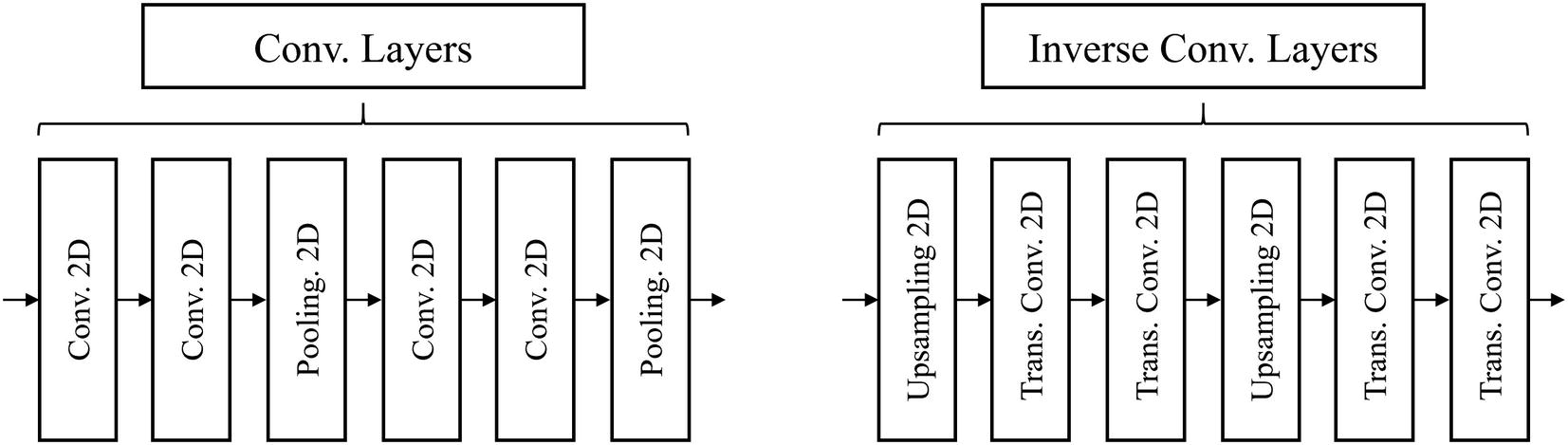
Example repeated module/cell-based design in convolutional autoencoders
However, when using convolutional layers in conjunction with pooling, we run into the problem of image sizes not divisible by the pooling factor. For instance, consider an image of shape (64, 64, 3). After a convolutional layer with filter size (2, 2) is applied to it, the image has a new shape of (63, 63, 3). If we want to apply pooling with size (2, 2) to it, we need to use padding in order to determine if the output of pooling will be (31, 31, 3) or (32, 32, 3). This is hardly a concern with standard convolutional neural networks. However, in autoencoders, we need to consider not only operations in the encoder but also the corresponding inverse “undoing” operations in the decoder. The upsampling layer has no padding layer. Thus, if we applied upsampling with size (2, 2) to an image with size (31, 31, 3), we would obtain an image of size (62, 62, 3); if we applied it to an image with size (32, 32, 3), we would obtain an image of size (64, 64, 3). In this case, there is no easy way in which we can obtain the original image size of (63, 63, 3).
You could attempt to work with specific padding and add padding layers manually, but it’s a lot of work and difficult to manipulate and organize systematically.
To address this problem, one approach of building convolutional autoencoders with pooling and convolutional layers is to use padding='same' on all convolutional layers. This means that convolutional layers have no effect on the shape of the image – images are padded on the side before the convolution is performed such that the input and output images have identical shapes. The convolution is still changing the content of the image, but the image size remains constant. Removing the effect of convolutional layers significantly simplifies the management of image shape. Beyond this simplification, padding also allows for convolutions to process features on the edge of the image that might be passed over without padding by adding more buffer room such that edge features can be processed by the center of the kernel.
The architecture of an example convolutional encoder with pooling and padding, using a vector-based bottleneck
Complete convolutional encoder with pooling and padding
The architecture of an example convolutional decoder with pooling and padding, using a vector-based bottleneck
Complete convolutional decoder with pooling and padding
This method, of course, relies upon your input having a certain size. In this case, the input size must be a power of 2, since each pooling factor decreases the image’s spatial dimensions by a factor of 2. You can insert a reshaping layer right after the input or reshape your dataset to accommodate this. The primary advantage of this method is that it makes organizing the symmetry of shape transformation much more simpler. If you know you want the shape of the encoded image right before flattening to be (16, 16, x)3, for instance, and that you want to have three pooling layers with size (2,2) and three pooling layers with size (3,3), you can calculate the corresponding input shape to be of 16 · 23 · 33 pixels in width and height.
Autoencoders for Other Data Forms
Using this logic, you can build autoencoders for data of all forms. For instance, you can use recurrent layers to encode and decode text forms of data, as long as an exact inverse decoding layer exists for every encoding layer you add. Although much of autoencoder work has been based around images, recent work is exploring the many applications of autoencoders for non-image-based data types. See the third case study in this chapter for an example of autoencoder applications in non-image data.
Autoencoder Applications
As we’ve seen, the concept of the autoencoder is relatively simple. Because of the need to keep the input and output the same size, however, we’ve seen that implementing autoencoder architectures for complex data forms can require a significant amount of forethought and pre-planning. The good news, though, is that implementing the autoencoder architecture is – in most autoencoders – the most time-intensive step. Once the autoencoder structure has been built (with the preferred compartmentalized design), you can easily adapt it for several applications to suit your purposes.
Using Autoencoders for Denoising
The purpose of denoising autoencoders is largely implied by its name: the “de” prefix in this context means “away” or “opposite,” and thus denoising is to move “opposite of” or to remove noise. Denoising is simple to implement and can be used for many purposes.
Intuition and Theory
In a standard autoencoder, the model is trained to reconstruct whatever input it is given. A denoising autoencoder is the same, but the model must reconstruct a denoised version of a noisy input (Figure 3-15). Whereas the encoder in a standard autoencoder only needs to develop a representation of the input image that can be decoded with low reconstruction error (which can be very difficult as is), the encoder in a denoising autoencoder must also develop a representation that is robust to any noise. Denoising autoencoders can be applied to denoise messy signals, images, text, tabular data, and other forms of data.
Denoising autoencoders are often abbreviated as DAE. You may notice that this is in conflict with the abbreviation of “deep autoencoder.” Because the term “denoising autoencoders” is relatively more established and clearly defined than “deep autoencoder,” when you see the abbreviation “DAE” in most contexts, it should be safe to assume that it refers to a denoising autoencoder. For the sake of clarity, in this book, we will favor not using the abbreviation “DAE”; if it is used, it will refer to the denoising autoencoder rather than the deep autoencoder.
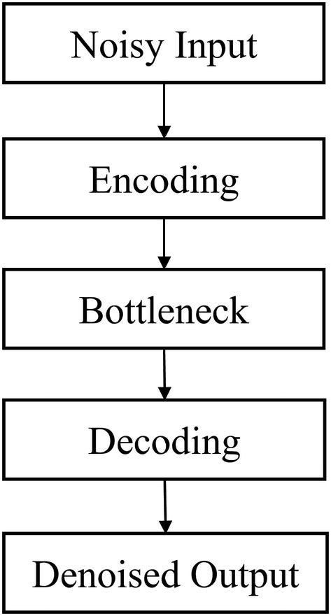
Conceptual diagram of the components of a denoising autoencoder
Of course, the concept of the denoising autoencoder assumes that your data is relatively free from noise in the first place. Because the denoising autoencoder relies upon the original data as the ground truth to perform denoising on the noisy version of that original data, if the original data is heavily noisy itself, the autoencoder will learn heavily arbitrary and noisy representation procedures. If the data you are using to train the denoising autoencoder has a high degree of noise, in many cases, there is little difference between using a denoising autoencoder and a standard autoencoder. In fact, using the former may be more damaging to your workflow because you may be operating under the assumption that the denoising autoencoder is learning meaningful representations of the data robust to noise when this is not true.
Apply noise as a layer: Insert a random noise-adding layer directly after the input of the autoencoder such that the noise is applied to the input before any encoding and decoding is performed on it. The primary advantage of this method is that the model learns to be robust to multiple noisy versions of the same original image, since each time the model is passed through the model, different noise is applied. However, the noise-adding layer needs to be removed before the denoising autoencoder is used in application; it only serves as an artificial instrument during training, and in application, we expect the input to already be “naturally” noisy. When using this method, you can create the dataset like you would create it for an autoencoder – the input and outputs are the same.
Apply noise to the dataset directly: Before training, apply noise to the dataset directly during its construction such that the data contains x as noisy data and y as the original data. The primary advantage of using this method is customizability: you can use any functions you would like to construct the dataset, since it is outside the scope of the neural network and therefore not subject to the restrictions of Keras and TensorFlow. You may want to add complex forms of noise that are not available as default layers or generators in Keras/TensorFlow. Moreover, there is no need to manipulate individual noise-adding layers of the autoencoder. However, you run the risk of overfitting (especially with small datasets and large architectures), because the autoencoder only sees one noisy form of each original input instance. Of course, you could manually produce several noisy forms of each instance, although it may take more time and be less efficient.
Apply noise through a data generator: Keras/TensorFlow contains an ImageDataGenerator object that can perform a variety of augmentations and other forms of noise to the image, like adjusting the brightness, making small rotations and shears, or distorting the hue. Moreover, the image data generator is similar to the layer-based method in that the network is exposed to many different noisy representations of the input data – data is passed through the random generator in each feed-forward motion and distorted before it is formally processed by the network. The primary advantage of using the data generator is that you can apply forms of noise that are more natural or expected to occur in the data than with layers, which can implement more “artificial” forms of noise like adding Gaussian noise to the image. Moreover, there is no need to manipulate noise-adding layers after training the denoising autoencoder. However, image data generators are limited only to images, which means you will need to use another method for other forms of data.
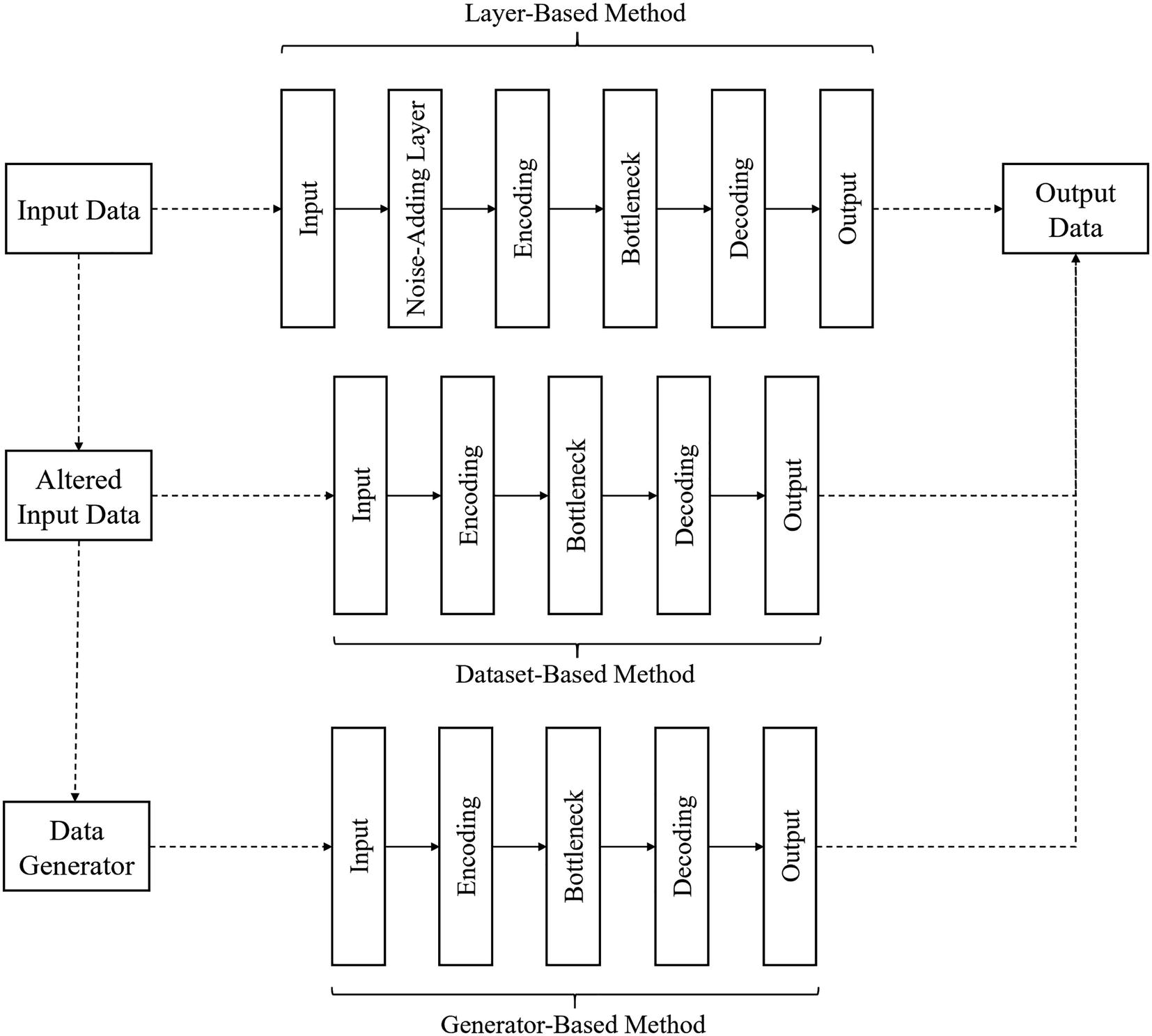
Three methods of inducing noise in a denoising autoencoder
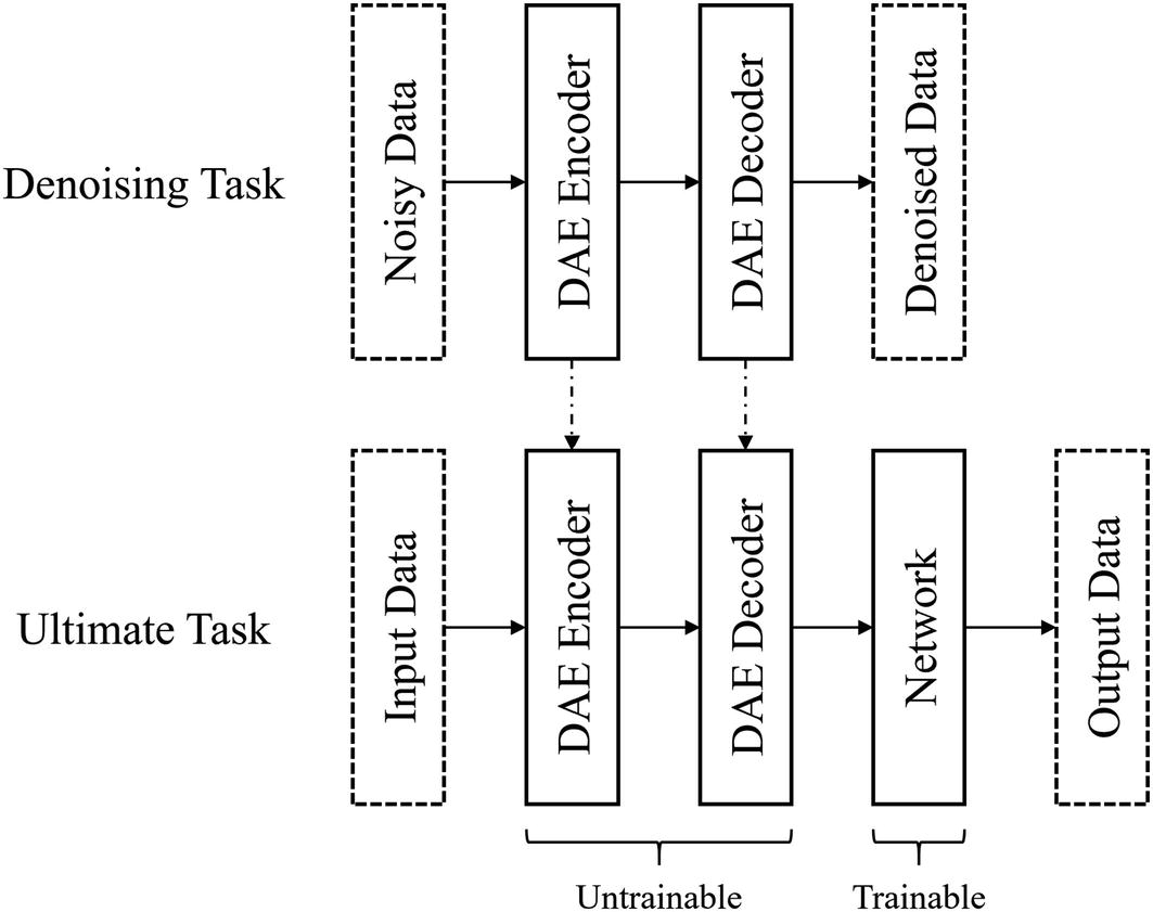
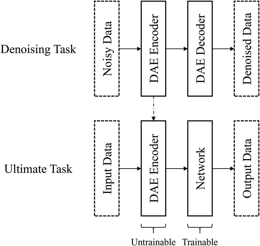
One method of using denoising autoencoders to perform denoising on input data before the denoised input is processed. You can also unfreeze the denoising autoencoder to fine-tune afterward
Consider a task in which a model must classify the sound of an audio input. For example, the model should be able to output a representation of the label “bird” if the audio input is of a bird song, or it should be able to output a representation of the label “lion” if the audio input is of a lion’s roar. As one may imagine, a challenge in this dataset of real-life audio is that many of the audio inputs will contain overlapping sounds. For instance, if the audio clip of the bird song was from a park surrounded by the metropolitan bustle, the background would contain sounds of cars driving and people talking. To be successful, a model will need to be able to remove these sources of background noise and isolate the core, primary sound.
To do this, say you obtain another dataset of real-life sounds without background noise. You artificially add some form of noise that resembles the noise you would encounter in the noisy dataset. For instance, you can use audio processing libraries in Python to overlay a sound without background noise with smaller, dimmed down background noise. It is key for the success of the denoising autoencoder that the noise you artificially generate resembles the expected form of noise in the data. Adding Gaussian noise to images, for instance, may not help much as a denoising task unless the dataset you would like to denoise contains Gaussian noise. (You may find that adding some form of noise is better than adding no noise at all in terms of creating a self-supervised pretraining task, but this will be discussed more later.) You train a denoising autoencoder to reconstruct the original unnoisy sound signal from the noise-overlayed signal and then use the denoising autoencoder to denoise real-life sounds before they are classified.
Denoising can occur in other forms, though, too. For instance, you can denoise the entire dataset with the denoising autoencoder before training a model on the ultimate task instead of architecturally inserting the denoising autoencoder into the model operating on the ultimate task. This could be successful if you expect the “ultimate” model to be applied to relatively clean data in deployment, but know that the training data available is noisy. It’s important to understand your particular problem well so you can successfully implement and manipulate your denoising autoencoder design.
Implementation
In our discussion of the implementation of denoising autoencoders, we will assume the autoencoder is being used for tabular data. The logic and syntax still can be applied to the use of denoising autoencoders for other data, like image or sequence data, with the necessary considerations for that particular data format.
Inducing Noise
As discussed, there are three practical methods of inducing noise.
Layer-based method of inducing noise into a denoising autoencoder
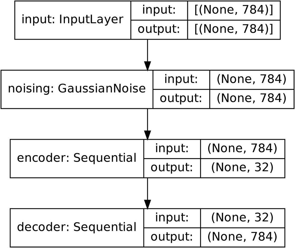
Example implementation of inducing noise via layer method
Another method of inducing noise is to apply it to the dataset directly, ideally during parsing when creating a TensorFlow dataset (Listing 3-15). When creating the parsing function, you can use a variety of TensorFlow image operations to induce random forms of noise. In this example, the unparsed TensorFlow dataset consists of a filename and a label for each instance (although you may find it helpful to arrange the unparsed dataset in another format if you know you will only use it for unsupervised learning).
Example function to pre-alter the dataset with noise using .map() on a TensorFlow dataset
Using the Image Data Generator method of inducing noise into an image dataset. Substitute augmentation_params for augmentation parameters. See Chapter 1 for a detailed discussion of Image Data Generator usage
You can also use ImageDataGenerator with class_mode='input' as an alternative data source for autoencoders generally (not just for denoising) instead of using TensorFlow datasets. If you do decide to use image data generators for autoencoders, be sure to be careful with how you control your augmentation parameters for your particular purpose. If you are training a standard autoencoder, for instance, in which the input is identical to the ideal output, make sure to eliminate all sources of artificial noise by adjusting the augmentation parameters accordingly.
Using Denoising Autoencoders
Removing the noise-inducing layer in a denoising autoencoder
Alternate method of removing the noise-inducing layer in a denoising autoencoder
Keep in mind that there are complications with this sort of method when using nonlinear topologies.
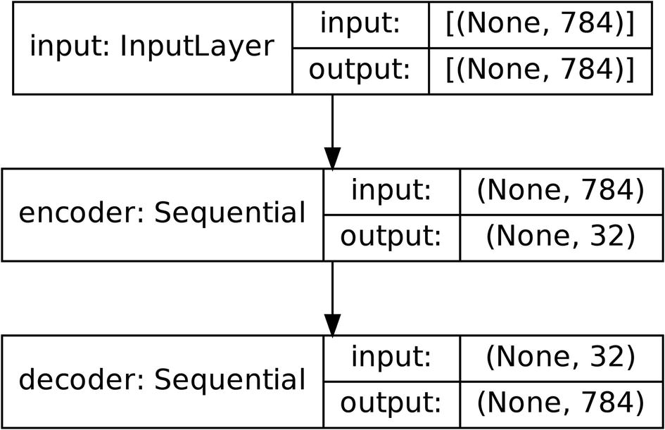
The denoising autoencoder after removing the Gaussian noise layer
Using a denoising autoencoder to denoise inputs before they are passed onto another model for further processing
Using the denoising autoencoder to decode the input before it is passed to the following layers for processing
You can set your own layer freezing strategy (see Chapter 2) as necessary to suit your own purposes. For instance, you may decide to freeze the weights in the denoising autoencoder for the majority of training and then to unfreeze the entire network and perform some fine-tuning afterward.
Using Autoencoders for Pretraining
Another application of autoencoders is for pretraining. Recall that pretraining is used to provide “context” such that it develops certain skills or representations that allow it to succeed in performing its ultimate task. In Chapter 2, we discussed various pretraining methods and strategies. We will build upon this prior discussion to demonstrate when and how to use autoencoders in the context of pretraining. With both extensive knowledge of autoencoders and of pretraining at this point, you will find that the intuition and implementation of autoencoders for pretraining is quite straightforward.
Intuition
The use of autoencoders in pretraining falls under the category of self-supervised learning. You could think of autoencoders as the simplest form of self-supervised learning. Recall that in self-supervised learning, a model is trained on an altered dataset, which is constructed only on the input data, not the labels, of the task dataset. Some self-supervised learning tasks, for instance, involve predicting the degree by which an image was rotated or the degree of noise that was added to some set of data. In a standard autoencoder, however, no alterations to the data are needed beyond moving data instances into a dataset such that the input and output are the same for each instance.
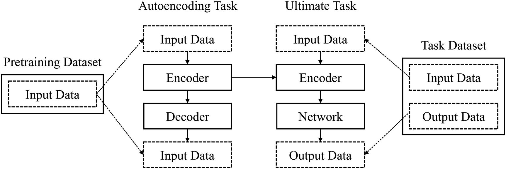
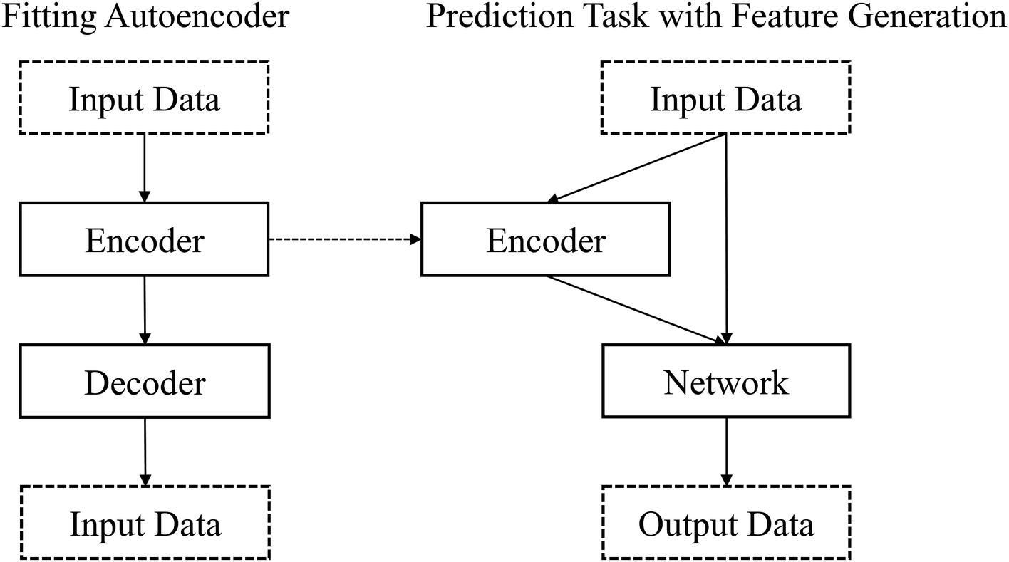
Conceptual map of using autoencoders for pretraining. Input data is the same for autoencoders. “network” is used to refer to the layers appended to the encoder. This isn’t entirely accurate, but it represents the idea that there is another “mini-network” that processes the output of the encoder to map whatever encoded representation comes out of the encoder into the output
If you plan to use an autoencoder for pretraining, it’s important you consider a key factor in how large to build the bottleneck (and correspondingly the widths of the encoder and the decoder components): the amount of information the layers appended after the encoder have to work with. If your bottleneck is large, the task may be trivial, and the network may not develop meaningful representations and processes for understanding the input. In this case, the processing layers after the encoder would receive a high number of features, but each feature would not contain much valuable information. On the other hand, if the bottleneck is too small, the model may develop meaningful representations, but the following processing layers may not have enough features to work with. This is a balancing process that takes experience and experimentation.
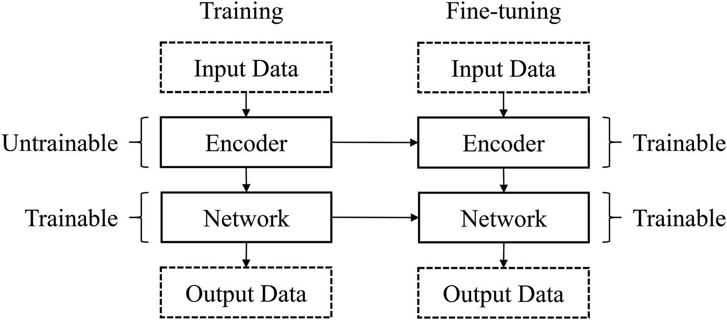
How components of the autoencoder for pretraining are frozen or unfrozen throughout training and fine-tuning
If you are using this method of pretraining with autoencoders with image data and you follow the design of flattening and reshaping the data around the bottleneck such that the bottleneck is a vector rather than an image, you will find that the structure of data transformation is especially clean. The encoder converts an image into a vector, and the following processing component processes that vector (which contains the encoded representation of the input) into the desired output. Thus, in this context, the encoder functions as the convolutional component and the following processing layers function as the fully connected component of an image-based deep learning model. This not only increases conceptual and organizational clarity but also allows you to further manipulate these sorts of autoencoder for pretraining designs for greater performance with the tools of transfer learning (see Chapter 2).
Note that while using autoencoders for pretraining, you can use a wide variety of autoencoder training structures beyond the standard autoencoder, in which the input is equivalent to the desired output.
Example of using non-standard autoencoder tasks for pretraining, like denoising autoencoder
However, when you are choosing the self-supervised task to train your autoencoder, it’s important to have a strong conceptual understanding of what that self-supervised task will accomplish. In this self-supervised context, the denoising autoencoder offers primarily a strong understanding of key features of the data, developed by identifying and correcting artificially inserted noise, and only secondarily actual denoising capabilities. This means that you do not need to be as careful about ensuring that the artificial noise resembles the true noise in the dataset when developing denoising autoencoders for pretraining. Of course, being conscious about the setup of the denoising autoencoder can allow you to maximize both the benefit of denoising (i.e., the encoder develops representations more or less robust to noise) and self-supervised learning (i.e., the encoder develops abstract representations of key features and ideas by learning to separate noisy artifacts from true meaningful objects).
It should be noted that the concepts of denoising and self-supervised learning are not completely independent from one another. To properly denoise an input, a model must develop representations of key features and concepts within the input, which is the goal of self-supervised learning.
This sort of simplicity and conceptual ease in manipulating autoencoders for pretraining makes them exceptionally popular in modern deep learning design.
Implementation
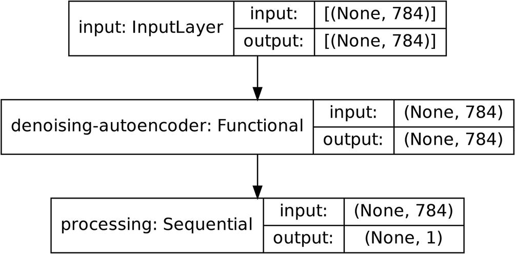
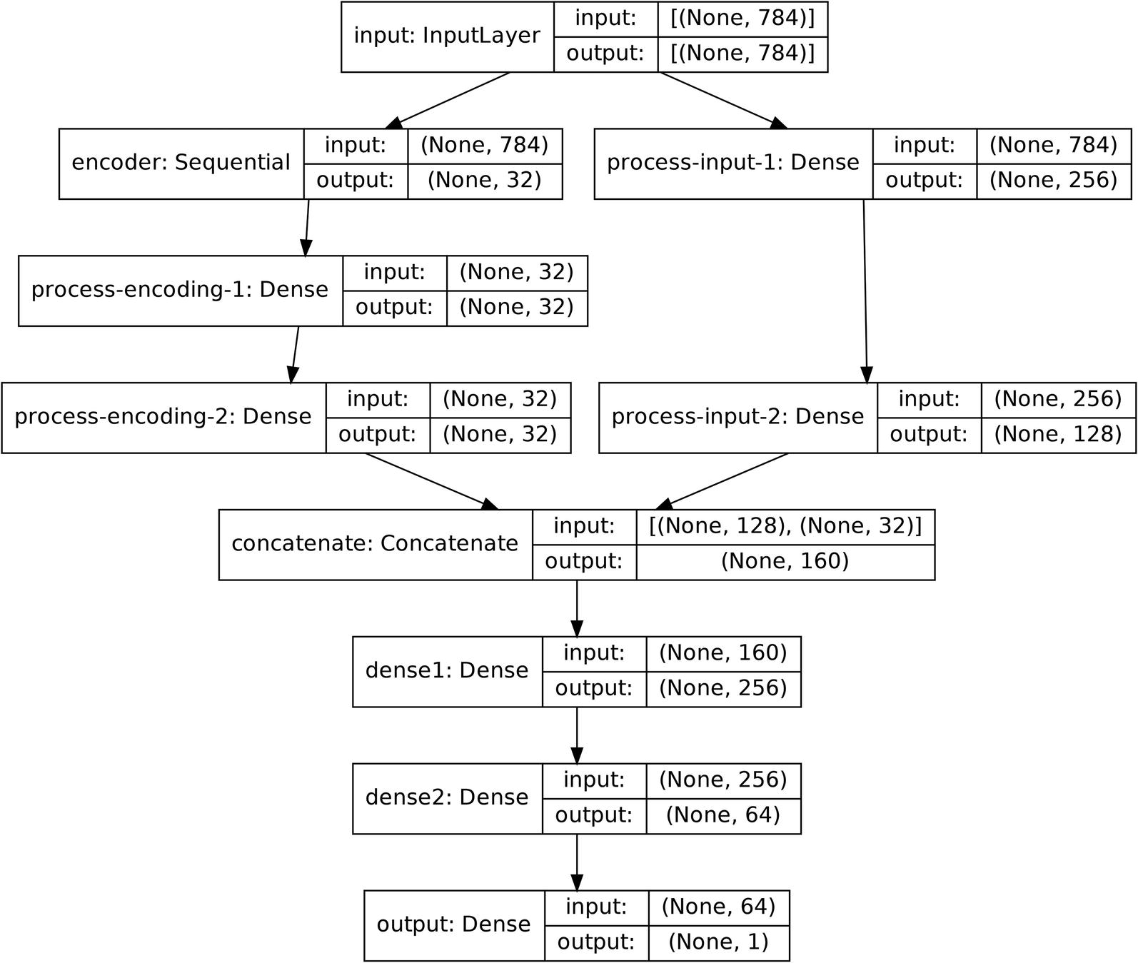
Implementing autoencoders for pretraining is simple, given that you have used compartmentalized design. Recall the autoencoder structure built to demonstrate the construction of autoencoders for tabular data, which took in data with 784 features and compressed it into 32 neurons in the bottleneck layer before reconstructing the 784 features.
Building a sub-model to process the outputs of the encoded features
Using the processing sub-model with the encoder in an overarching model for a supervised task
Make sure to freeze layers as appropriate.
Using Autoencoders for Dimensionality Reduction
The concept of the autoencoder was initially presented as a method of dimensionality reduction. Because the application of dimensionality reduction is almost “built into” the design of the autoencoder, you will find that using autoencoders for dimensionality reduction is very simple to implement. However, there’s still much to consider in performing dimensionality reduction for autoencoders; with the right design, autoencoders can offer a unique method of dimensionality reduction that is more powerful and versatile than other existing methods.
Intuition
Dimensionality reduction is generally performed as an unsupervised task, in which data must be represented with a smaller number of dimensions than it currently exists in. Many dimensionality reduction algorithms like Principal Component Analysis (PCA) and t-Stochastic Neighbor Embedding (t-SNE) attempt to project data into lower spaces according to certain mathematical articulations of what features of the data should be valued most in a reduction. PCA attempts to preserve the global variance, for instance, while t-SNE instead seeks to capture the local variance. Because different dimensionality reduction algorithms are built to prioritize the preservation of different features of the data, they are fundamentally different in character and thus are limited in their effectiveness on a wide variety of datasets.
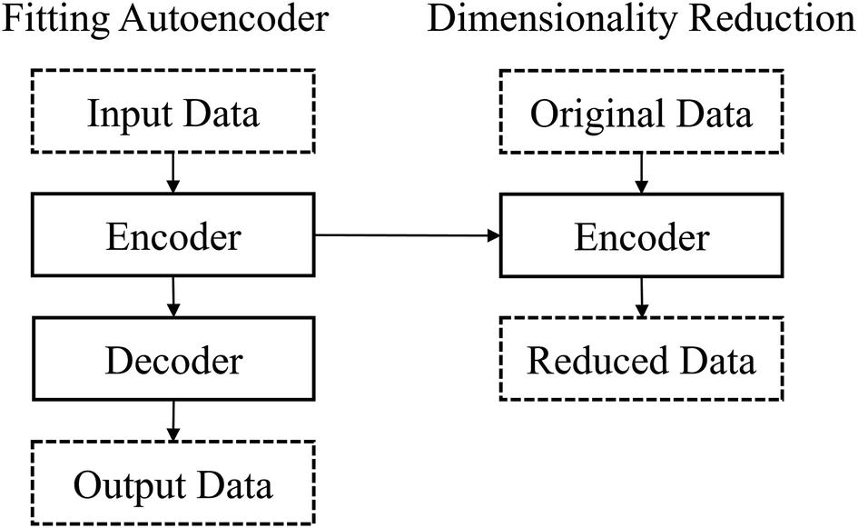
Conceptual map of using autoencoders for dimensionality reduction
Adaptability: Algorithms like PCA and t-SNE allow the user to adapt the algorithm to their dataset by manipulating a few parameters, but that quantity is vastly outnumbered by the adaptability of the autoencoder. Because autoencoders are more of a concept than an algorithm, they can be built with a much greater degree of adaptation to your particular problem. You can change the depth and width of the autoencoder structure, the activations in each layer, the loss function, regularization, and many other features of neural network architectural and training design to change how an autoencoder behaves in performing dimensionality reduction. This also means that using autoencoders for dimensionality reduction is likely to be successful only if you are aware of how different manipulations to the autoencoder structure translate to changes in its behavior and the behavior of a dimensionality reduction algorithm necessary to handle dimensionality reduction on your dataset.
Articulation of valued features : Autoencoders prioritize certain features of the data and optimize the reduction of data in a way different from algorithms like PCA and t-SNE in character. Autoencoders attempt to minimize the reconstruction loss, while PCA and t-SNE attempt to maximize some relatively explicit mathematical formulation of what to prioritize, like the preservation of local or global structure (e.g., variance). These formulations attempt to capture what “information” entails in the context of dimensionality reduction. On the other hand, autoencoders do not seem, at least on the surface level, to have these prioritizations built explicitly into their design – they simply use whatever reduction allows for the most reliable reconstruction of the original input. Perhaps autoencoders are one of the most faithful representatives to capturing “information” in a broad, conceptual sense – rather than being tied toward any particular explicit assumptions of what constitutes a preservation of information (i.e., the means of preservation), it adopts whatever procedures and assumptions are necessary for the original item to be reconstructed (i.e., using whatever means are necessary to obtain optimal ends of preservation).
These two features can both be advantages and disadvantages. For instance, adaptability can be a curse rather than a tool if your dataset is too complex or difficult to understand. Moreover, increased adaptability does not necessarily suggest increased interpretability of adaptation; that is, while the autoencoder possesses a much wider range of possible behaviors, it is not necessarily simple to identify which changes to the architecture will correspond to certain changes (or absence of changes). Note that the autoencoder’s articulation of valued features is determined by its loss function, which uses as one component the model prediction, which depends on the model architecture (among other modeling details). Finding your way through this chain of considerations is likely more arduous a task than adjusting relatively interpretable parameters on other dimensionality reduction methods.
Modern autoencoders for dimensionality reduction are most often used on very high-dimensional data since deep learning has evolved to be most successful on complex forms of data. More traditional algorithms like PCA developed for the reduction of lower-dimensional data are unlikely to be suited toward data like word embeddings in NLP-based models and high-resolution images. t-SNE is a popular choice for high-dimensional data, but primarily for the purpose of visualization. If you are looking to maximize the information richness of a dimensionality reduction and are willing to sacrifice some interpretability, autoencoders are generally the way to go.
Implementation
Using autoencoders for dimensionality reduction requires no further code from building and training the original autoencoder (see previous sections on building autoencoders for tabular and two-dimensional data). Assuming the autoencoder was built with compartmentalized design, you can simply call encoder.predict(input_data), where encoder corresponds to the encoder architecture and input_data represents the data you would like encoded.
Using Autoencoders for Feature Generation
Feature generation and feature engineering is often thought of as a relic of classical machine learning, in which engineering a handful of new features could boost the performance of machine learning models. In deep learning applications involving relatively more complex forms of data, however, in many cases, using standard feature engineering methods like finding the row-wise mean of a group of columns or binning is unsuccessful or provides minimal improvement.
With autoencoders, however, we are able to perform feature generation for deep learning using an entity with the power and depth of deep learning methods.
Intuition
The encoding component of the autoencoder can be used to generate new features for a model to take in and process when performing a task. Because the encoder has learned to take in a standard input and compress it such that each feature in the encoded representation contains the most important information from the standard input, these encoded features can be exploited to aid the prediction of another model.
Functionally, the idea is almost identical to autoencoders for dimensionality reduction. However, using autoencoders for feature generation requires the additional step of generating new features and feeding the new features into the model.
We’ve seen earlier that a similar concept is employed in using autoencoders for pretraining, in which the encoder is detached from a trained autoencoder and inserted directly after the input of another network, such that the component(s) of the model after the encoder receive enriched, key features and representations of the input. However, the purpose of feature generation is to generate, or add, features rather than replacing them. Thus, when using autoencoders for feature generation, the encoder provides one set of encoded, information-rich features that are considered alongside the original set of features.
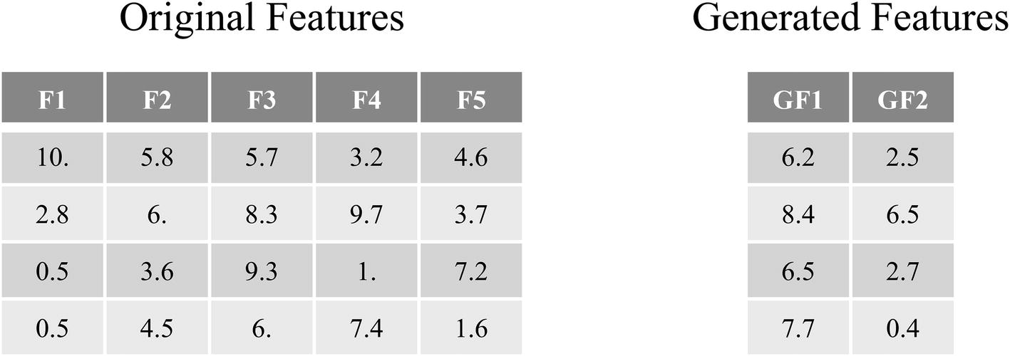
Hypothetical datasets: original features and the generated features (produced by the output of an encoder in a trained autoencoder). The exact numbers in these tables are hypothetical (randomly generated)
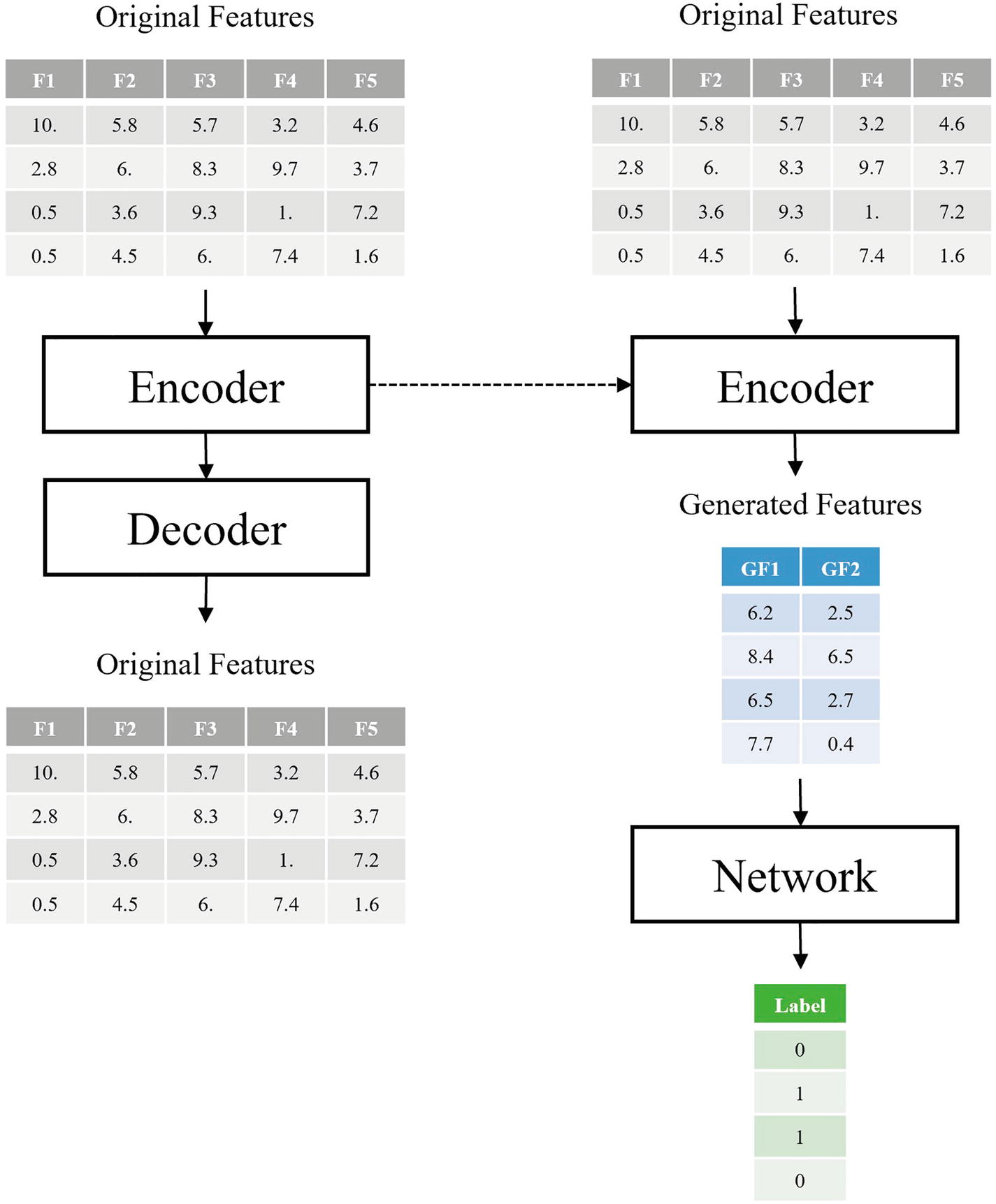
Using only generated features from the encoder as inputs to the network
However, a concern arises from this particular approach: even though the encoder from the autoencoder will almost always give the model a boost (if designed and trained properly), does the encoder impose a limit on the performance of the model by forcing it to take information strictly through the lenses of the autoencoder? Sometimes, a bit of fine-tuning after training (in which the encoder weights are unfrozen and the entire model is trained) is enough to resolve this concern.
Even fine-tuning may not be an adequate address of this concern, though, in several circumstances. If the autoencoder does not obtain a relatively high performance in reconstruction (i.e., middling, mediocre performance), forcing the model only to take in mediocre-level features could limit its performance. Alternatively, if the data is not of extremely high complexity, like tabular data or lower-resolution images, having an encoder compress the original inputs may be valuable, but not completely necessary. In many cases, models intended for less complex data benefit from processing both the original input and encoded features.
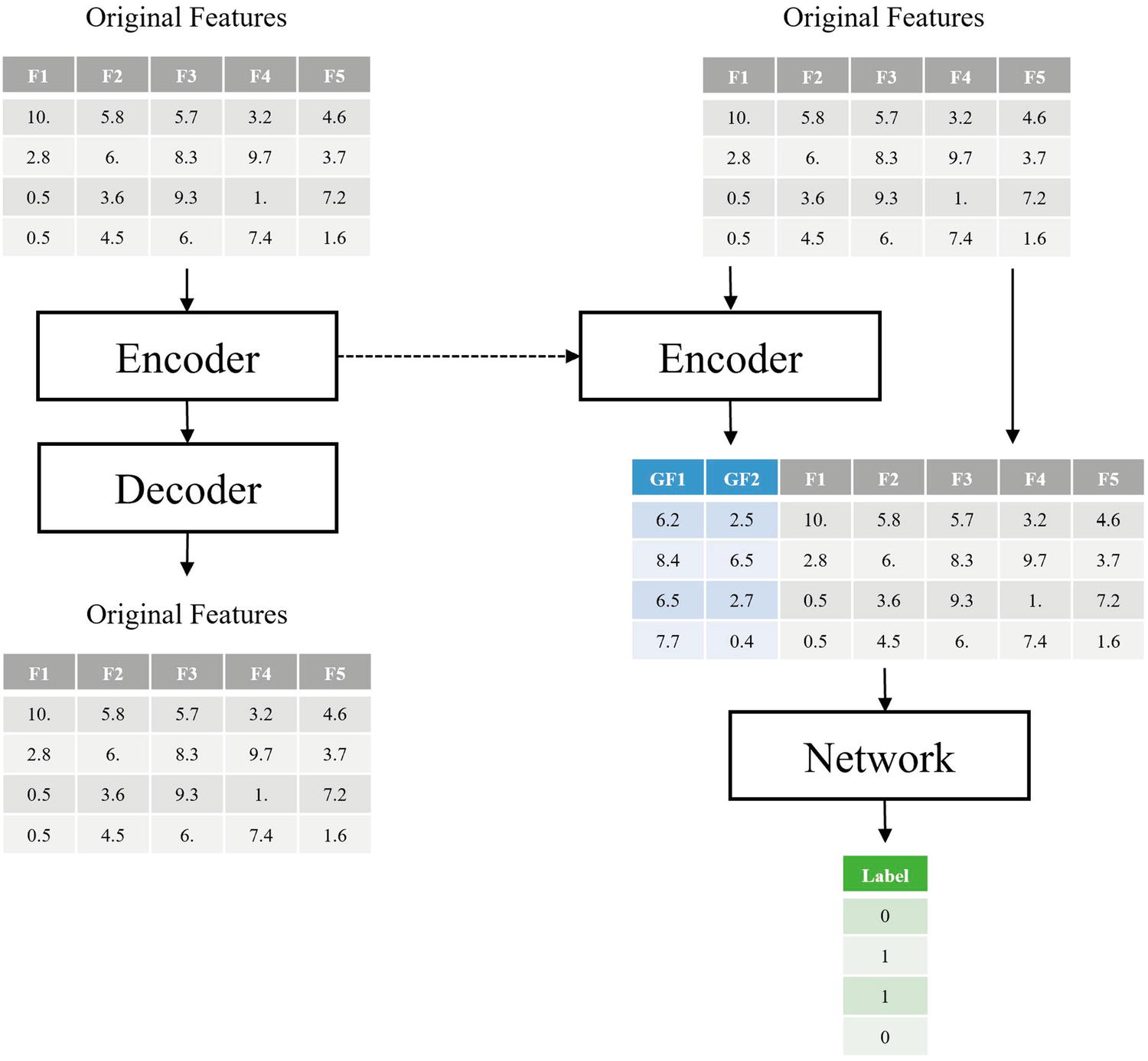
Using both generated features from the encoder and original features as inputs to the network
Conceptual map of how fitted autoencoders can be used in a prediction task with feature generation in which both the original features and the generated features are inputted to the remaining network layers for processing
This is similar in character to the layer-based method of inducing noise when training a variational autoencoder. You could pass data through the encoder and concatenate the encoded features to the original dataset and then feed the merged dataset into a standard network architecture. However, such an approach, in which changes to the data are performed outside of the neural network, is doing more work than necessary – it’s much easier to use the Functional API to add the encoder than to get messy with predictions and data organization, especially if your dataset is on the larger side. Adding the encoder model directly into the new model automatically puts these relationships and data flows in place.
Implementation
Creating the feature generation component of the autoencoder, in which inputs are passed through the encoder and concatenated to those outputs
Processing the concatenated features
Hypothetical map of the architecture of an autoencoder used for feature generation
Be sure to set encoding.trainable = False, as the encoder’s weights – the basis for the method by which it extracts core features and representations – should be frozen during training. The need for fine-tuning is less significant than if the autoencoder were used for pretraining.
Processing the encoded representation and the original input separately before they are concatenated
Hypothetical map of the architecture of an autoencoder used for feature generation with further processing on the output of the encoder and the original features before concatenation
Broadly, you can use these sorts of architectural manipulations to build all sorts of complex nonlinear topologies to take advantage of pretraining methods.
Using Variational Autoencoders for Data Generation
The variational autoencoder is one of the more modern conceptions of the autoencoder. It serves a relatively recent developing subfield in deep learning: data generation. While variational autoencoders are most often employed in the generation of images, they also have applications in generating language data and tabular data. Although image generation can be used to generate photorealistic images, more practically variational autoencoders are often used to generate more data to train another model on, which can be useful for small datasets. Because variational autoencoders heavily rely upon the notion of a latent space, they allow us to manipulate their output by traversing the latent space in certain ways. This allows it to offer more control and stability in the generated outputs than other data generation methods, like Generative Adversarial Networks (GANs).
Intuition
The goal of an autoencoder is to reconstruct the original input data as identically as possible. On the other hand, the goal of the variational autoencoder is to produce a similar image with reasonable variations – hence, the name “variational” autoencoder.
The fundamental idea behind generation using the variational autoencoder isn’t too complex: not only individual points within the latent space (corresponding to data points in the dataset) are meaningfully arranged so that they can be decoded into their original form, but the latent space itself – consisting of all the space in and around existing data points – is mapped to by the encoder such that it contains relationships relevant to the dataset. Therefore, we can sample points from the latent space not occupied by existing encoded representations of data points from the dataset and decode them to generate a new data item that wasn’t part of the original dataset.
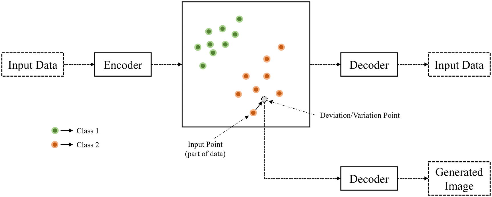
Decoding regions of the latent space near the latent space point of a data point to generate variations of the data – data that is different, but that shares similar features. The box in the center represents the latent space – the points in the bottleneck region to which input data has been mapped to and which will be mapped back into a reconstructed version
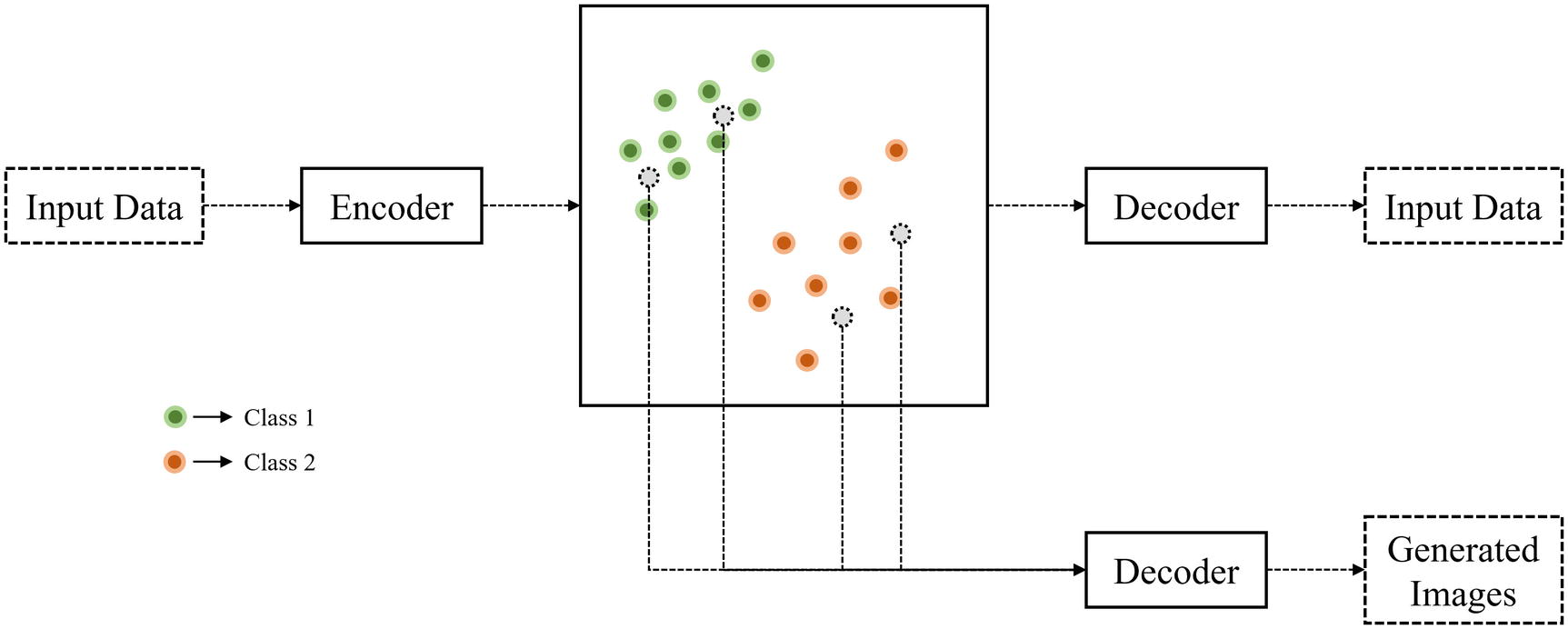
Sampling randomly from the latent space to produce a wide, diverse dataset of generated data
- 1.
Train an autoencoder on a reconstruction task.
- 2.
Randomly select several points in the latent space, either by making changes to existing data points (ensuring that it is within a reasonable domain).
- 3.
Decode each of those points into the respective generated image.
While this general logic and intuition is valid, there is a problem with an assumption we have made: with standard autoencoders, the latent space is not continuous; rather, it’s much more likely to be heavily discrete, separated into clusters. Continuity is unlikely to be helpful in the task of reconstructing inputs, because it magnifies the effect of small “slips” and “mistakes”; rather, having a discrete design allows for some minimum “guarantee” of success (Figure 3-33).
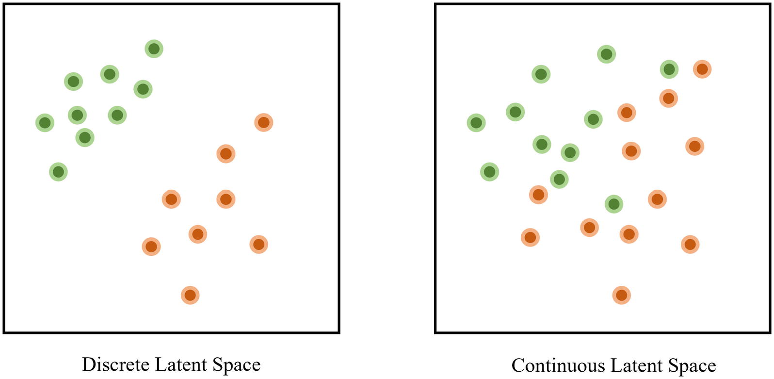
A discrete vs. continuous latent space in autoencoders
On the other hand, assume the latent space is continuous, meaning that there are no purposeful gaps separating clusters of images. If there is a similar deviation in the positioning of an encoded image containing the digit “0,” it may be reconstructed by the decoder as “1” – there is no gap, or barrier, that separates the concepts of “0” and “1” from each other.
Thus, discreteness within autoencoders is a useful tool for autoencoders to improve the performance of their reconstruction by sectioning off main ideas. It has been empirically observed that successful autoencoders tend to produce discrete latent spaces.
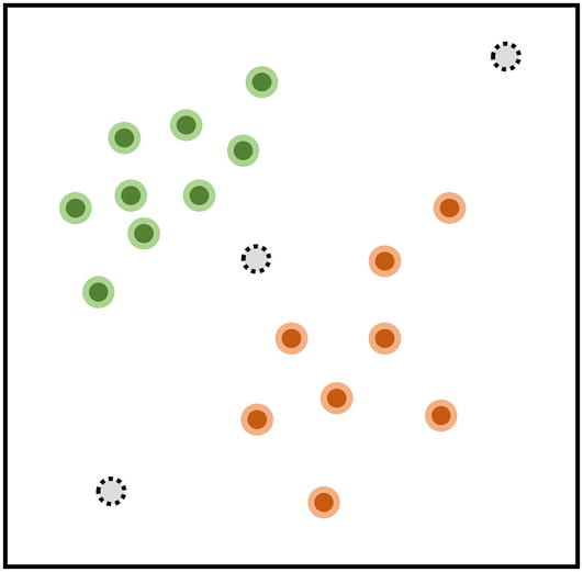
Sampling from “gap” regions of the latent space that the decoder has not learned to decode leads to bizarre and wildly unrealistic inputs
You may hypothesize that decoding a randomly sampled point in this “gap” would result in some sort of image that is “in between” both of the classes. However, the decoder has never been exposed to points in the latent space from that region and therefore does not have the experience and knowledge to interpret it. Therefore, the decoder will likely output some sort of gibberish that is in no way related to the original dataset.
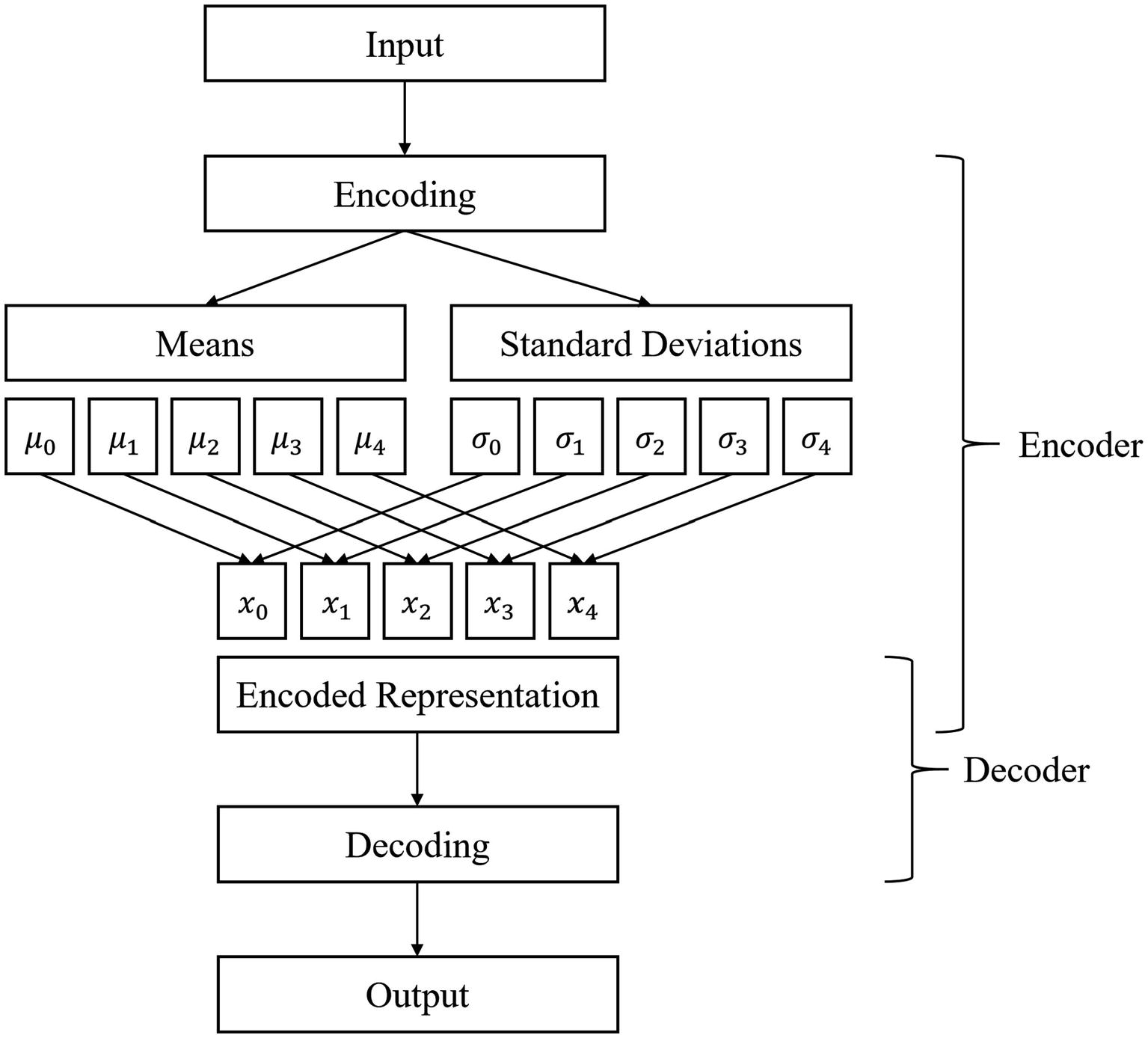
The encoder learns the optimal mean and standard deviation of variables in the latent space, from which an encoded representation is sampled and passed on to the decoder for decoding.
The variational autoencoder is optimized on a custom loss function: a blend of reconstruction loss (this is the cross-entropy, mean squared error, or any other standard autoencoder loss function used) and KL divergence to prevent the model from “cheating” (more on this “cheating” later).
Architecture of a variational autoencoder
The architecture of the variational autoencoder exposes a certain beauty in deep learning: we can profoundly shape the neural network’s thinking processes to our own desires with a few well-placed nudges. For instance, you may be wondering: what if certain latent variables aren’t normally distributed? Over time, the network will adapt the encoding and decoding processes to accommodate the normal distribution because we use the normal distribution assumption to choose the encoded representation. If it did not adapt, it would not attain optimal performance. We can expect the variational autoencoder to learn this adaptation with high certainty because modern neural networks possess reliably high processing power. This, in turn, allows us to more freely impose (reasonable) expectations within models as a means to accomplish some end.
Similarly, even though we would like the branches after encoding to represent the means and standard deviations of the latent variables, we don’t build any hands-on mechanisms before these two branches to manually tell the network what the mean or standard deviation is. Rather, we assume that each of the branches takes the role of the mean and the standard deviation of a distribution when generating the encoded representation (the expectation) and allow the network to adapt to that expectation. This sort of expectation-based design allows you to implement deep learning ideas faster and more easily.
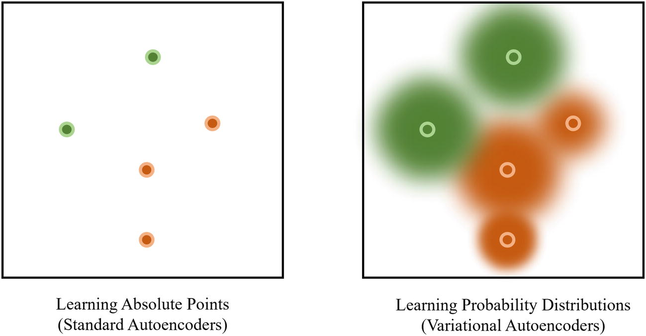
Standard autoencoders learn the absolute locations of data in the latent space, whereas variational autoencoders learn probability distributions
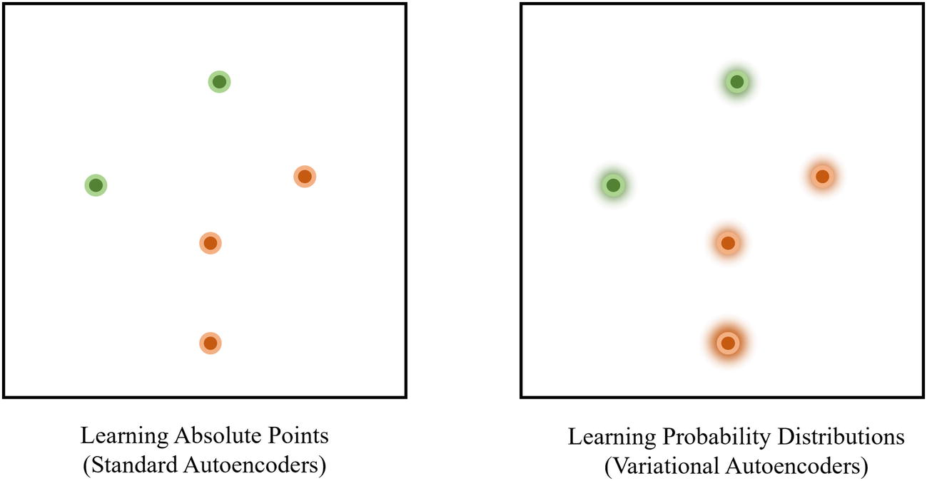
In practice, variational autoencoders can “cheat” and replicate the absolute point learning of standard autoencoders by forming clustering patterns and reducing the standard deviation
KL divergence, or Kullback-Leibler divergence, measures the level of divergence, or difference, between two probability distributions (roughly speaking). For the purposes of variational autoencoders, KL divergence is minimized when the mean is 0 and the standard deviation is 1 and thus acts as a regularization term, punishing the network for clustering or reducing the standard deviation.
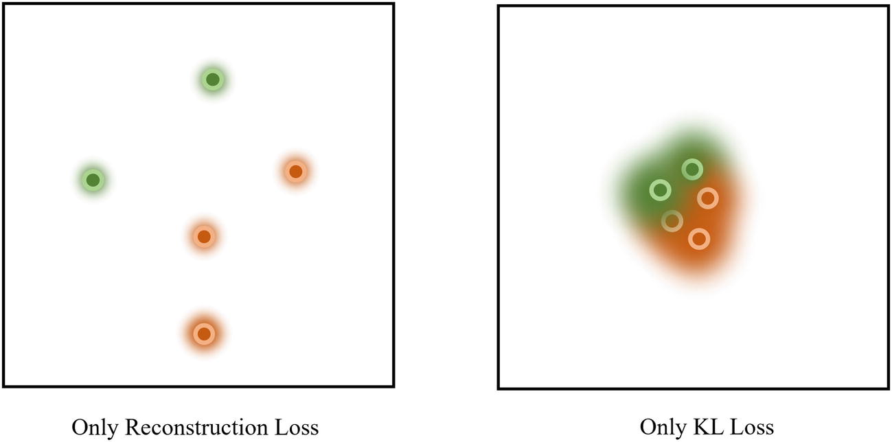
Results of latent space representations when only using reconstruction loss vs. only using KL loss
To address this problem, variational autoencoders are trained on the sum of reconstruction loss and KL loss. Thus, the variational autoencoder must simultaneously develop encoded representations that can be decoded into the original representation but will be punished if the representations make use of clustering, low standard deviations, and other marks of a discrete space. The variational autoencoder is a unique model in that its objective cannot be clearly articulated by any one existing loss function and thus is formulated as a combination of two functions.
Now, you can random uniformly sample the latent space within the domain of learned representations and produce both a diverse and realistic set of generated images. Moreover, our intuitive logic of interpolation applies: if you want to visualize what lies “in between” two images (e.g., a cat and a dog or the digit “1” and “9”), you can find the point in between the corresponding two points in the latent space and decode it.
Implementation
Implementing variational autoencoders is more difficult than implementing other autoencoder applications, because we need to access and manipulate components within the autoencoder itself (the latent space), whereas prior the only significant step was to change the input and output flow. Luckily, this serves as a useful exercise in the construction of more complex neural network structures in Keras.
Recall that in the Functional API, each layer is assigned to a variable. Although you should always be careful and specific with your variable naming, this is especially true with complex and nonlinear neural network architectures like the variational autoencoder. You’ll need to keep track of the relationships between several layers across several components, so establish a naming convention and code organization that works best for you. If you make mistakes, you’ll run into graph construction errors. Frequently use plot_model with show_shapes=True if you need guidance in debugging these errors to show what went wrong.
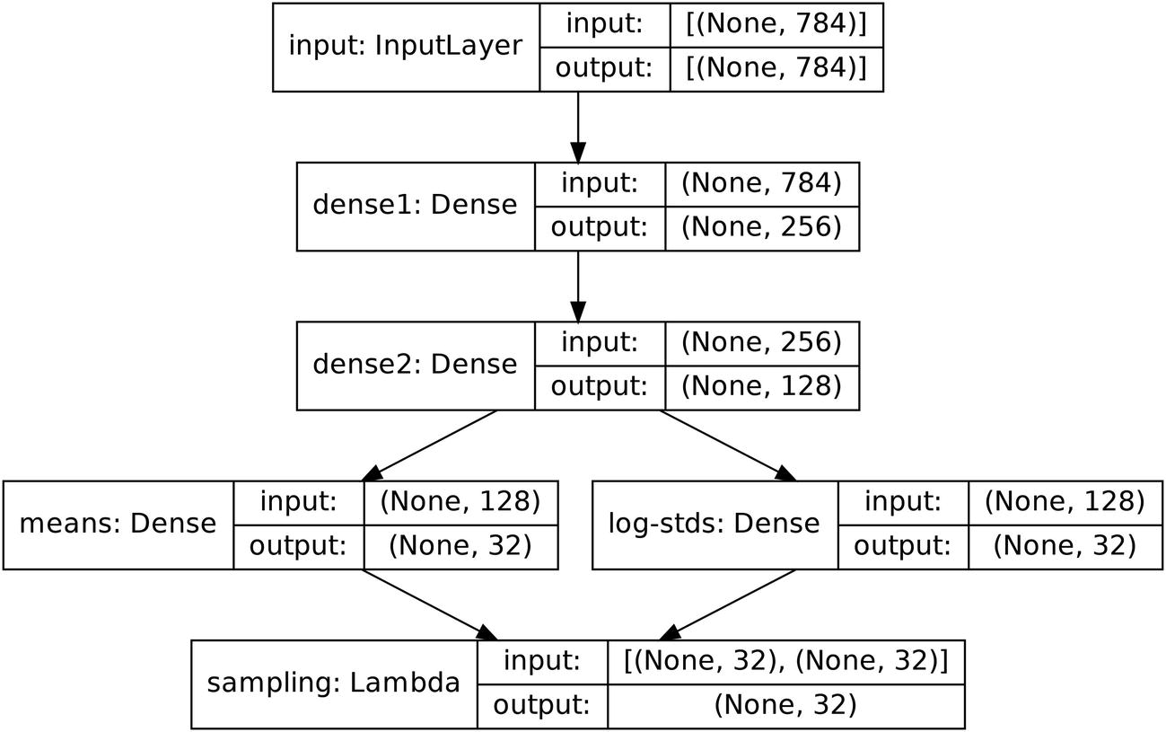
Implementing the first layers of the encoder for a variational autoencoder
Creating the branches to represent the mean and log standard deviations of the latent variable distributions
We’ve built two branches, representing the mean and log standard deviation of the latent variable distributions. In this case, our latent space has 32 dimensions (like a standard autoencoder with 32 bottleneck nodes), with one mean value and one log standard deviation value to describe the distribution. To attain the output of the encoder – the encoded representation of the input – we need to take in both the mean and the standard deviation, randomly sample from that distribution, and output that random sample (Listing 3-27). This sort of operation isn’t built as a default layer in Keras/TensorFlow, so we’re going to have to build it ourselves.
Structure of creating a custom layer that performs TensorFlow operations on inputs using Lambda layers
In this example, custom_layer takes in the outputs of two previous layers. However, Keras delivers this data together in one argument variable containing all of the arguments to the custom function, which can be unpacked within the custom function. Additionally, all operations must be Keras/TensorFlow operations (see Keras backend for Keras’ low-level operations). Note that you can use methods like TensorFlow’s py_func (see Chapter 1) to convert Python functions into TensorFlow operations, if necessary.
Creating a custom layer to sample encoded representations from the mean and log standard deviations of latent variables
The shape parameter used in creating the epsilon variable is expressed in this example as (tf.shape(means)[0], 32). Alternative methods include (tf.shape(log_stds)[0], 32) and (tf.shape(means)[0], tf.shape(means)[1]): all capture the same idea. In order for the actual sampling (μ + σ · ϵ) to be successful, the tensors for the mean, standard deviation/log standard deviation, and epsilon normally distributed randomness need to be the same size. Because this data is one-dimensional, we know that the input shapes to the sampling layer will be in the form of (batch_size, latent_space_size). We haven’t specified what the batch size is, so we simply used tf.shape(mean)[0]. However, we know the latent space size – 32 dimensions. With more complex data types, it’s important to understand the shape of the inputs to this sampling data you’re dealing with.
It should also be noted that while the mean with which the epsilon tensor is generated should remain at 0, the standard deviation can be changed depending on how much variation you’re willing to introduce. More variation could allow the model to better interpolate and produce more realistic and diverse results, but too much could risk introducing too much noise to possibly be plausibly decoded. On the other hand, less variation allows the decoder to better decode the image but may result in less exploration and smooth interpolation of “gaps” in the latent space.
Aggregating the encoder model
Building the encoder of the variational autoencoder
Creating and aggregating the decoder model
Aggregating the encoder and decoder sub-models into an overarching variational autoencoder model
This method of combining components together into a model is like the method that has been used for standard autoencoders with two key differences. Firstly, the input to the variational autoencoder is not a unique keras.layers.Input or keras.Input input mechanism, but the input to the encoder (enc_inputs). This is because of the design of the variational autoencoder’s loss function: because the model must have access to the output of the encoder, the encoder’s input must also be on the same “level” as the variational autoencoder itself. Note that this is a valid operation because we’re not making any actual architectural changes (i.e., rerouting layers or adding multiple branches to one layer), only simplifying a technically redundant (but perhaps organizationally helpful) process of passing data through two input layers. Secondly, the decoder does not take in the entire encoder output, but instead indexes it (decoded = decoder(encoded[2])). Recall that for the KL divergence component of the loss function to have access to the distribution parameters, the encoder outputs the tensors containing the mean and log standard deviation, as well as the actual encoded representation. The decoder only takes in the encoded representation, which is the third output of the encoder, and is thus indexed accordingly.
Building the reconstruction loss component of the variational autoencoder’s custom loss function
Building the KL divergence loss component of the variational autoencoder’s custom loss function
Note that tf.reduce_sum allows you to sum the losses for each item across a specified axis; this is necessary to deal with batching, in which there is more than one data point per batch.
Combining reconstruction and KL divergence loss into the VAE loss
We need to make one more accommodation for the variational autoencoder’s unique loss function: usually, the loss function is passed into the model’s .compile() function . However, we can’t do this in this case because the inputs to our loss function are not predictions and ground truth labels that the Keras data flow assumes loss functions take in when passed through compiling: instead, it takes in the outputs of specific layers. Because of this, we use vae.add_loss(vae_loss) to attach the loss function to the variational autoencoder.
The model can then be compiled (without the loss function, which has already been attached) and fitted on the data. Since there are so many crucial parameters that determine the behavior of the variational autoencoder (architecture size, sampling standard deviation, etc.), it’s likely that you’ll need to tweak the model parameters a few times before you reach relatively optimal performance.
We’ve taken several measures to adapt our model structure and implementation to work with the unique nature of the variational autoencoder’s loss function. While this book – and many tutorials – will present the building of these sorts of architectures in a linear format, the actual process of constructing these models is anything but sequential. The only way to truly know if the unique situation you are working with requires a certain workaround or needs to be rewritten or re-expressed somehow is to experiment. In this case, it is likely helpful to first write down the basic architectures of the encoder and the decoder, implement the custom loss function, and then test and experiment which changes to the architecture and/or loss function are needed to make it all work, consulting documentation and online forums as necessary.
Case Studies
In these case studies, we will discuss the usage of autoencoders for a wide variety of applications in recent research. Some can be accessed via existing implementations, whereas others may be out of the reach of our current implementation skills – nevertheless, these case studies provide rich and interesting examples of the versatility of autoencoders and put forth empirical evidence of their relevance in modern deep learning.
Autoencoders for Pretraining Case Study: TabNet
Deep learning is quite famously seldom used for tabular data. A common critique is that deep learning is “overkill” for simpler tabular datasets, in which the massive fitting power of a neural network overfits on a dataset without developing any meaningful representations. Often, tree-based machine learning models and frameworks like XGBoost, LightGBM, and CatBoost are employed instead to handle tabular data.
However, especially with larger tabular datasets, deep learning has a lot to offer. Its complexity allows it to use tabular data in a multimodal fashion (considering tabular data alongside image, text, and other data), engineer features optimally on its own, and use tabular data in deep learning domains like generative modeling and semi-supervised learning (see Chapter 7).
End-to-end design: TabNet does not need feature processing and other preprocessing methods required when using tabular data for other approaches.
Sequential attention: Attention is a mechanism that is commonly used in language models to allow the model to develop and understand relationships between various entities in a sequence. In TabNet, sequential attention allows the model to choose, at each step, which features it should consider. This, moreover, allows for greater interpretability of the model’s decision-making processes.
Unsupervised pretraining : TabNet is pretrained using an autoencoder-based architecture to predict masked column values in a tabular fashion. This leads to a significant performance and improvement. TabNet demonstrated, for the first time, large improvement from self-supervised pretraining on tabular data.
For the purposes of this case study, the unsupervised pretraining via autoencoder structure is the focus.
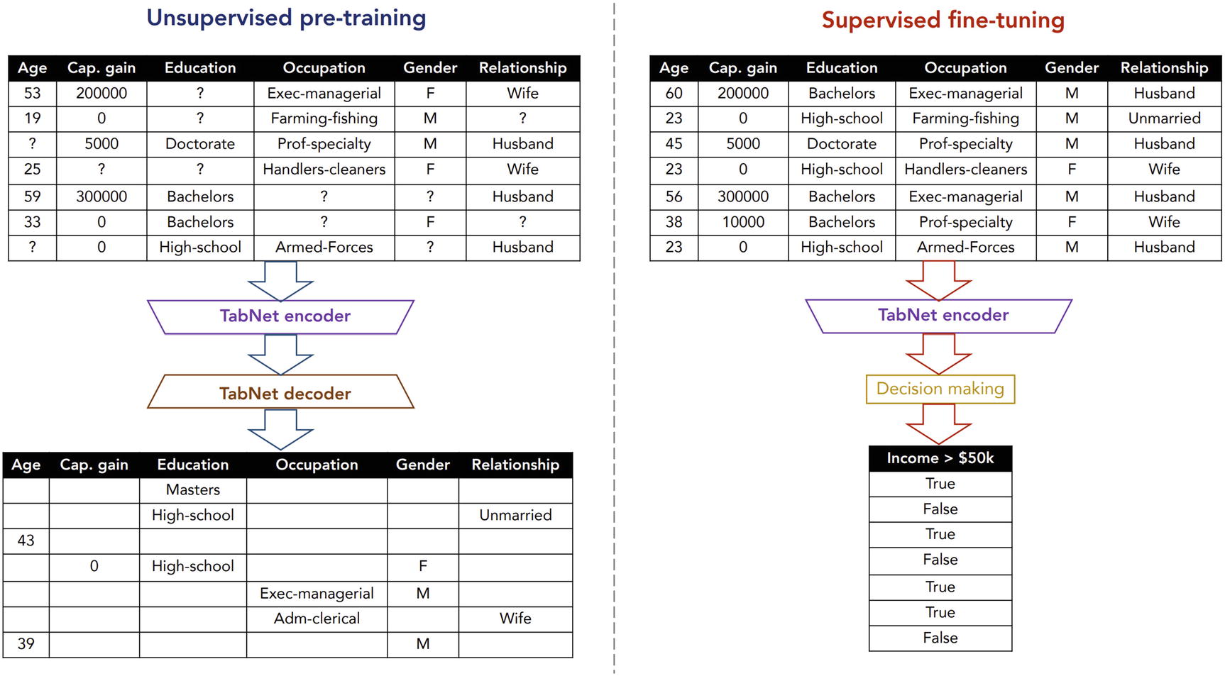
TabNet method of unsupervised pretraining before supervised fine-tuning. Produced by Arik and Pfister
Performance on Forest Cover Type dataset
Model | Test Accuracy (%) |
|---|---|
XGBoost | 89.34 |
LightGBM | 89.28 |
CatBoost | 85.14 |
AutoML Tables | 94.95 |
TabNet | 96.99 |
Performance on the Sarcos dataset
Model | Test MSE | Model Size |
|---|---|---|
Random forest | 2.39 | 16.7 K |
Stochastic decision tree | 2.11 | 28 K |
MLP | 2.13 | 0.14 M |
Adaptive neural tree | 1.23 | 0.60 M |
Gradient boosted tree | 1.44 | 0.99 M |
Small TabNet | 1.25 | 6.3 K |
Medium TabNet | 0.28 | 0.59 M |
Large TabNet | 0.14 | 1.75 M |
Performance on the Higgs Boson dataset with the medium-sized TabNet model. Similar improvements with pretraining are observed with other databases
Training Dataset Size | Test Accuracy (%) | |
|---|---|---|
Without Pretraining | With Pretraining | |
1 K | 57.47 ± 1.78 | 61.37 ± 0.88 |
10 K | 66.66 ± 0.88 | 68.06 ± 0.39 |
100 K | 72.92 ± 0.21 | 73.19 ± 0.15 |
To work with the TabNet model, install the tabnet library with pip install tabnet. Two relevant ready-to-go TabNet models are implemented: tabnet.TabNetClassifier and tabnet.TabNetRegressor, for classification and regression tasks, respectively (Listing 3-35). These models can be compiled and fitted like standard Keras models.
Instantiating a TabNet classifier from the tabnet library
It is important to fit the model with a high initial learning rate that gradually decays and a large batch size anywhere between 1% and 10% of the training dataset size, memory permitting. See the documentation for information on syntax for more specific modeling.
Denoising Autoencoders Case Study: Chinese Spelling Checker
English , like many other European languages, relies upon the piecing together of letter-like entities sequentially to form words. Misspelling in English can be addressed relatively well with simple rule-based methods, in which a rulebook maps common misspelled words into their correct spellings. Deep learning models, however, are able to consider the context of the surrounding text to make more informed decisions about what word the user intended to use, as well as fix grammar mistakes and other language errors.
However, Chinese “words” are characters rather than strings of letters. Mistakes in Chinese are commonly the result of two primary errors: visual similarity (two characters share similar visual features) and phonological similarity (two characters are pronounced similarly or identically). Because Chinese and English have different structures and therefore different requirements for correcting spelling, many of the deep learning approaches adapted for English and other European languages cannot be readily transferable to Chinese.
In “FASPell: A Fast, Adaptable, Simple, Powerful Chinese Spell Checker Based on DAE-Decoder Paradigm,” Yuzhong Hong, Xianguo Yu, Neng He, Nan Liu, and Junhui Liu5 propose a deep learning approach to correcting Chinese spelling based upon the denoising autoencoder architecture.
The approach consists of two components: a masked language model and a confidence-similarity decoder. The masked language model takes in sample text and outputs several candidates for replacement. The confidence-similarity decoder selects replacements from these candidates to form the completed, spell-checked sentence.
Standard masking : Some fraction of the dataset uses the same random masking as BERT: some character(s) is masked with a [MASK] token, and the model predicts which character is masked based on the context. This is performed on texts that have no errors.
Error self-masking : Errors in the text are “masked” as themselves. The target label corresponds to the correct character. The model must identify that there is an error and perform a correction to obtain perfect performance.
Non-error self-masking : Correct characters in the text are also “masked” as themselves, and the target label is that character. This is to prevent overfitting. In this case, the model must identify that there is no error and allow it to pass through the model unchanged.
While the masked language model provides the basis for the spelling correction, on its own is a weak Chinese spell checker – the addition of the confidence-similarity decoder to improve performance.
The decoder attempts to process and understand the denoised candidates generated by the masked language model. The decoder takes in both the confidence of the masked language model in each character and the similarity between characters. The similarity between two characters is calculated as a combination of their visual and phonological similarity.
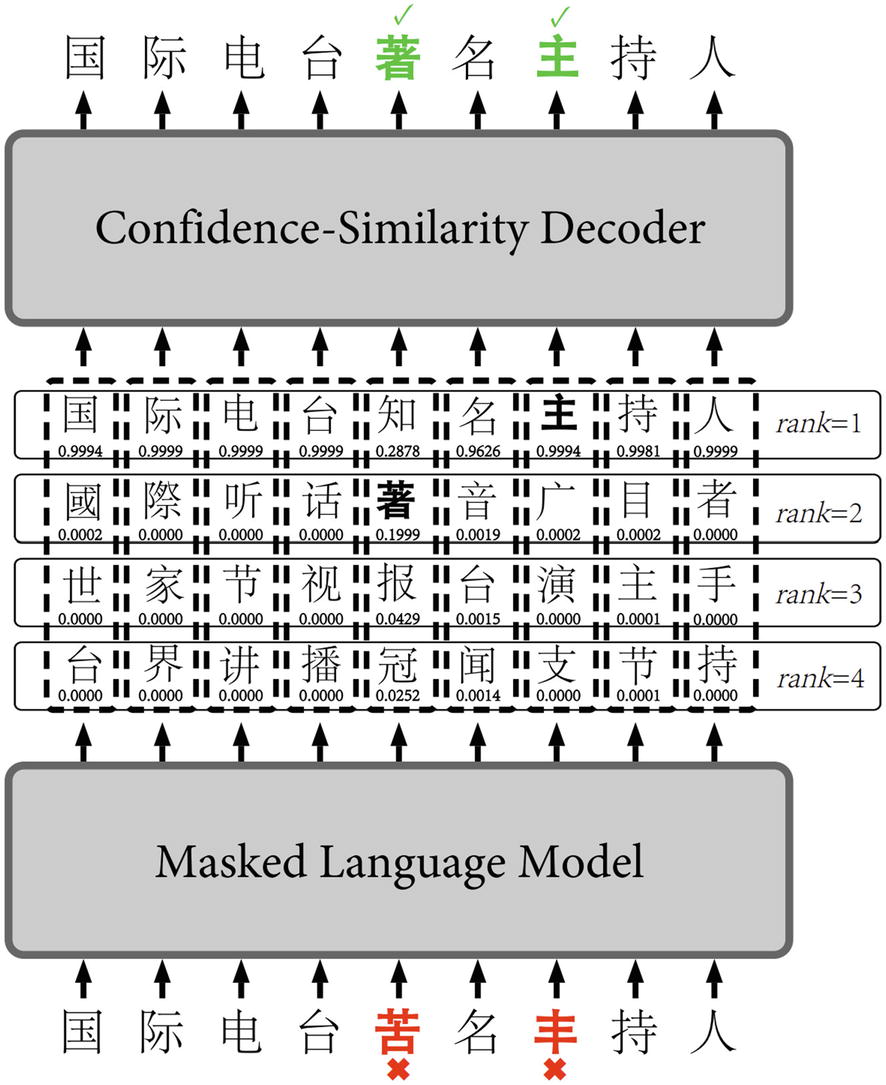
Architecture and example data flow throughout the FASPell model, including the masked language model and the confidence-similarity decoder. Produced by Hong et al
On the other hand, if the masked language model has a high confidence in a correction, but the correction and the original character have little similarity, these two signals must be closely compared. If the masked language model’s confidence is high enough as to outweigh the low similarity between the original character and the correction, the correction is accepted. For each character in the sentence, the correction that maximizes the model confidence and the similarity with the original character is accepted and inserted into the final output.
Performance of FASPell in various spelling tasks, measured with three different metrics
Model | Detection | Correction | ||||
|---|---|---|---|---|---|---|
Precision | Recall | F1 | Precision | Recall | F1 | |
Wang et al. | 54.0 | 69.3 | 60.7 | Not reported | Not reported | 52.1 |
Yeh et al. | Not reported | Not reported | Not reported | 70.3 | 62.5 | 66.2 |
FASPell | 76.2 | 63.2 | 69.1 | 73.1 | 60.5 | 66.2 |
Performance of versions of FASPell in various spelling tasks, measured with three different metrics
Model | Detection | Correction | ||||
|---|---|---|---|---|---|---|
Precision | Recall | F1 | Precision | Recall | F1 | |
FASPell | 76.2 | 63.2 | 69.1 | 73.1 | 60.5 | 66.2 |
FASPell without fine-tuning | 75.5 | 40.9 | 53.0 | 73.2 | 39.6 | 51.4 |
FASPell without confidence-similarity decoder | 42.3 | 41.1 | 41.6 | 32.2 | 31.3 | 31.8 |
FASPell without fine-tuning or confidence-similarity decoder | 65.2 | 47.8 | 55.2 | 48.4 | 35.4 | 40.9 |
FASPell shows the importance of adapting autoencoders toward your particular task. By changing the content and method by which the denoising autoencoder was trained and adding a confidence-similarity decoder to incorporate knowledge of character similarity into understanding the denoising autoencoder’s output, FASPell was able to address a key shortcoming in standard pretrained autoencoder designs.
Variational Autoencoders Case Study: Text Generation
Earlier , we looked at variational autoencoders for image data. Recall that variational autoencoders are especially valuable because we can control the generated data by making changes to the sampled location in the latent space. This allows for fine control over attributes like the text’s sentiment and writing style that is not possible with other generation methods.
Variational autoencoders generally work with the right design well on images. However, applying variational autoencoders for text generation, in which convolutional layers are replaced with recurrent layers, is more difficult. Recall that the loss for variational autoencoders is a sum of the reconstruction loss and KL divergence. KL divergence acts as a regularizing term that can be optimized by clustering the latent variable distributions closer together.
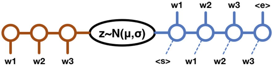
The traditional LSTM-based variational autoencoder for text generation, which suffers from KL divergence term collapse
The architecture includes a hybrid of convolutional and recurrent layers; the encoder is composed completely of convolutional layers, whereas the decoder combines deconvolutions (like transpose convolutions) and a traditional RNN. Deconvolutional layers were chosen instead of recurrent layers for two key reasons: deconvolutional layers have more efficient GPU implementations, and feed-forward architectures are easier to optimize than recurrent ones, due to a more consistent and smaller number of steps required.
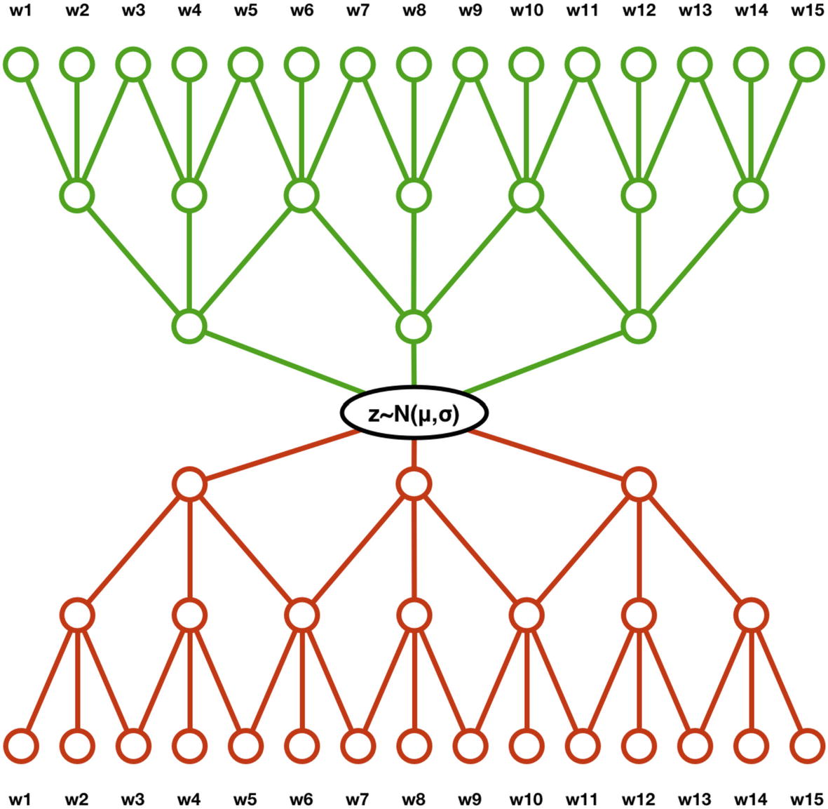
The feed-forward component of the variational autoencoder. Inputs enter through the bottom and are processed through convolutions and deconvolutions to produce a generated set of features
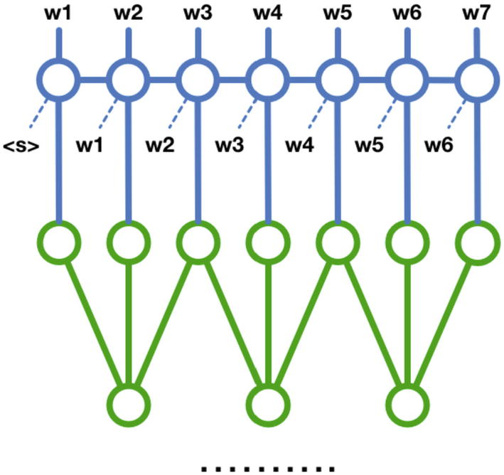
The LSTM component of the hybrid approach, in which the generated features are further decoded by an LSTM-style model into text to capture complex sequence-based dependencies between entities of a sentence
Input dropout: A dropout layer is applied to the input such that the input, even before encoding, is already corrupted in a random fashion.
KL term annealing: By gradually increasing the weight of the KL divergence term in the loss function across time, the neural network transitions from being a standard autoencoder into a variational autoencoder.
Auxiliary reconstruction term: A specialized term is added to the loss, which can be optimized only by meaningful reconstruction and encoding. This exacerbates the importance of the reconstruction component of the loss function.
Semeniuta, Severyn, and Barth’s work shows how being creative with combinations of layers and transgressing prepackaged boundaries for what certain model types should look like, in addition to well-pointed, specific mechanisms to target particular challenges, can lead to significantly greater performance.
Key Points
Autoencoders encode and decode data in the process developing important representations of the dataset and efficient processes for extracting key information and features from data. Autoencoders rely upon the context of the dataset to support their efficient representations. Therefore, while they are not good universal compression algorithms, they have many applications that exploit the autoencoder’s unique ability to learn complex relationships and representations of data in an unsupervised fashion.
A key trade-off in autoencoder design is the size of the bottleneck: a bottleneck that is too small may make any encoding task too difficult to be practical, whereas a bottleneck that is too large can be solved trivially without developing meaningful representations.
Use compartmentalized design when implementing autoencoders and other complex neural network structures by defining models as a series of relationships between sub-models. This makes implementing autoencoder applications significantly easier and is also conceptually more clear to mentally understand and manipulate.
To build an autoencoder for tabular data, simply stack Dense layers with a progressively decreasing number of neurons in the encoder and a progressively increasing number of neurons in the decoder. To build an autoencoder for image data, use convolutional layers and pooling layers in the encoder, and transpose convolutional layers and upsampling layers in the decoder. Convolutional autoencoders often flatten and reshape in the region surrounding the bottleneck such that the output of the encoder (the encoded representation) is a vector. Use padding='same' in convolutional layers for easy manipulation of the shape size. Autoencoders can also be built for other data types, as long as there exists an inverse decoding layer for every encoding layer.
Denoising autoencoders are autoencoders trained to reconstruct the original data from a corrupted, noisy input. If you are using denoising autoencoders to denoise dataset, ensure that the form of noise is realistic and exists within the dataset. When implementing denoising autoencoders, noise can be induced either as a layer, applied to the dataset, or as an Image Data Generator (in the case of images).
When using autoencoders for pretraining, the autoencoder is first trained on unsupervised data to extract key ideas and representations. Then, the encoder is detached and custom processing layers are added after it to alter the model structure such that it can perform a supervised task. The encoder weights are usually frozen such that the following layers can be trained to interpret the output of the encoded representations; this can be followed by some fine-tuning to optimize performance.
Autoencoders are different from other dimensionality reduction algorithms in two key ways: higher adaptability and a model-centric articulation of valued features. These can be implemented simply by having the encoder predict encoded representations for certain data inputs.
Using autoencoders for feature generation is like using them for dimensionality reduction, but the encoded features are concatenated to the original dataset rather than replacing the original dataset. This can be implemented with a nonlinear architecture, in which the input is both passed through the encoder and concatenated to the output of the encoder; this enriched data can then be passed through a series of processing layers to be interpreted and used to produce an output.
Variational autoencoders allow for the generation of new data by choosing locations in the latent space and decoding them. However, because standard autoencoders tend to produce discrete spaces that cannot be sampled randomly, variational autoencoders implement two key changes to force development of a continuous latent space: learning the probability distributions of latent variables rather than the absolute position and adding KL divergence to the loss function to provide regularization in the formation of the latent space. Variational autoencoders rely upon relatively more low-level operations but can be accomplished with good organization and active experimentation.
Autoencoders are extraordinarily versatile structures that you can work into almost any deep learning design. Keep them in mind when you approach a new deep learning problem and need somewhere to start – autoencoders provide a good starting point for developing knowledge and building important representations.
In the next chapter, we’ll discuss model compression and the exciting implications it holds for the future of deep learning.