
It is my ambition to say in 10 sentences what everyone else says in a book.
—Friedrich Nietzsche, Philosopher and Writer1
Over the course of deep learning’s flurried development in these recent decades, model compression has relatively recently become of prominent importance. Make no mistake – model compression methods have existed and have been documented for decades, but the focus for much of deep learning’s recent evolution was on expanding and increasing the size of deep learning models to increase their predictive power. Many modern convolutional networks today contain hundreds of millions of parameters, and Natural Language Processing models have reached hundreds of billions of parameters (and counting).
While these massive architectures push forward the boundaries of what deep learning can do, often their availability and feasibility are restricted to the realm of research laboratories and other high-powered departments within organizations that have the hardware and computational power to support such large operations. Model compression is concerned with pushing forward the “cost” of the model while retaining its performance as much as possible. Because model compression aims primarily at maximizing efficiency rather than performance, it is key to transferring deep learning advances from the research laboratory to practical applications like satellites and mobile phones.
Model compression is often a missing chapter in many deep learning guides, but it’s important to remember that deep learning models are increasingly being used in practical applications that impose limits on how wildly one can design the deep learning model. By studying model compression, you can ground the art of deep learning design in a practical framework for deployment and beyond.
Introduction to Model Compression
When we perform model compression, we attempt to decrease the “cost” a model incurs while maintaining its performance as much as possible. The term “cost” used here is deliberately vague because it encompasses many attributes. The most immediate cost of storing and manipulating a neural network is the number of parameters it holds. If a neural network contains hundreds of billions of parameters, it will take more storage than a network that contains tens of thousands of parameters. It will be unlikely that applications with lower storage capability, like mobile phones, can even feasibly store and run models on the larger end of modern deep learning designs. However, there are many other factors – all related to one another – that factor into the cost of running a deep learning model:
Since model compression is largely a concern of deployment, we’ll use the corresponding language: “server side” and “client side.” Roughly speaking, for the purposes of this book, “server side” refers to the computations performed on the servers servicing the client, whereas “client side” refers to the computations performed on the client’s local resources.
Latency: The latency of a deep learning model is the time taken to process one unit of data. Latency usually concerns the time it takes for a deployed deep learning model to make a prediction. For instance, if you’re using a deep learning algorithm to recommend search results or other items, a high latency means slow results. Slow results turn away users. Latency is usually correlated with the size of the model, since a larger model requires more time. However, the latency of a model can also be complicated by other factors, like the complexity of a computation (say a certain layer does not have many parameters but performs a complex, intensive computation or a heavily nonlinear topology).
Server-side computation and power cost : Computation is money! In many cases, the deep learning model is stored on the server end, which is continually calculating predictions and sending those predictions to the client. If your model is computationally expensive, it will incur heavy literal costs on the server side.
Privacy : This is an abstract but increasingly important factor in today’s technological landscape. Services that follow the preceding model of sending all user information to a centralized server for predictions (for instance, your video browsing history sent to a central server to recommend new videos, which are sent back to and displayed on your device) are increasingly subject to privacy concerns, since all user information is being stored at one point in a centralized location. New, distributed systems are increasingly being used (e.g., federated learning), in which a version of the model is sent to each user’s individual device and yields predictions for the user’s data without ever sending the user’s data to a centralized location. Of course, this requires the model to be sufficiently small to operate reasonably on a user’s device. Thus, a large model that cannot be used in distributed deployment can be considered to incur the cost of lack of privacy (Figure 4-1).

Privacy requires a small model. While it may not be completely quantifiable, it’s an important aspect of a model’s cost
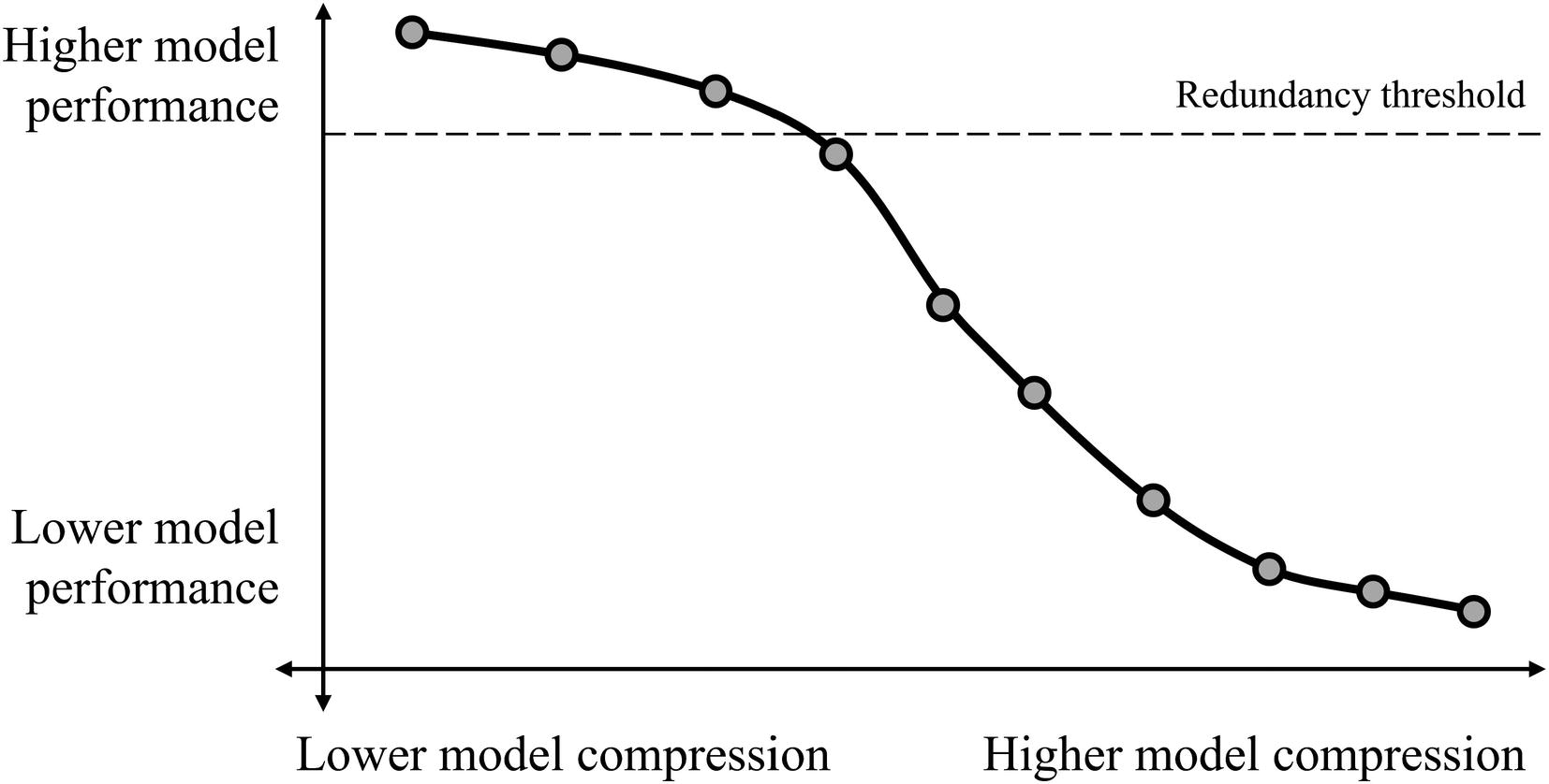
A hypothetical relationship between model performance and model compression, with a redundancy threshold – the threshold before continual model compression leads to a dramatic decrease in model performance – marked. The actual relationship may vary by context and model compression type
Which combination is optimal depends on your particular task and resource availability. Sometimes, performance is not a high priority compared to cost attributes. For instance, consider a deep learning model on a mobile application tasked with recommending apps or other items to open – here, it is much less important that the model be perfect than it is for the model to not consume much of the mobile phone’s storage and computation. It is likely that a user would be unsatisfied net-wise if such an application consumed much of their phone’s resources, even if such an application performed well. (In fact, deep learning may not even be the right approach in this situation – a simpler machine learning or statistical model may suffice.) On the other hand, consider a deep learning model built into a medical device designed to quickly diagnose and recommend medical action. It is likely more important for the model to be perfectly accurate than it is to be a few seconds faster.
Model compression is fascinating because it demonstrates the true breadth of problem-solving required to fully tackle a deep learning problem. Deep learning is not concerned only with improving model performance by the metrics but also about developing practical deep learning that can be used in real-life applications.
It also is valuable in advancing theoretical understandings of deep learning because it forces us to ask key questions about the nature of neural networks and deep learning: if model compression can so effectively remove much of the information from a network with a marginal decrease in performance, what purpose did the original component of the network that was compressed “away” serve in the first place? Is neural network training fundamentally a process of improving solutions by tuning weights or a process of discovery – finding a good solution in a sea of bad solutions? How fundamentally robust are networks to small variations? We’ll explore these questions along with a discussion on their benefits to practical deployment.
In this chapter, we will discuss three key deep learning model compression algorithms: pruning, quantization, and weight clustering. Other deep learning model compression/downsizing methods exist – notably, Neural Architecture Search (NAS). However, it is not discussed in this chapter because it is more appropriate in the next chapter.
Pruning
When you think of the number of parameters in a neural network, you likely associate parameters with the connections between nodes of each layer in a fully connected Dense network or perhaps the filter values in a convolutional neural network. When you call model.summary() and see the eight- or nine-figure parameter counts, you may ask: are all of those parameters necessary to the prediction problem?
As mentioned earlier, you can reasonably expect from simple reasoning that it is very likely you did not build a neural network architecture with the “perfect” number of parameters to succeed at its task, and thus if the network doesn’t underperform, it likely is using more parameters than it truly needs. Pruning is a direct way to address these “superfluous” parameters by explicitly removing them. Its success in all sorts of architectures, moreover, poses important questions in theoretical deep learning.
Pruning Theory and Intuition
Imagine that you want to cut down on comforts in your living space – you think that there might be more than you need to work and that keeping all the comforts is increasing your cost of living beyond what it could be. You’ve made changes in your living space with an eye toward minimally reducing the impact on your ability to work – you still keep your computer, good Wi-Fi, steady electricity. However, you’ve cut down on comforts that may aid your work but that are fundamentally auxiliary by removing or donating items like a television subscription, a nice couch, or tickets to the local symphony.
This change in living space shouldn’t theoretically impact your work, provided you are reasonably resilient – your mental facilities have not been explicitly damaged in a way that would impair your ability to perform the functions of work (perhaps it affects your comfort, but that’s not a factor in this discussion). Meanwhile, you’ve managed to cut down on general costs of living.
However, you’re a bit disoriented: you reach instinctively for a lamp in the corner that has been removed. You find yourself disappointed that you can’t watch unlimited television anymore. Making these changes to this space requires reorienting yourself to it. It takes a few hours (or even days) of exploration and orientation to acclimate toward these new changes. Once you have completed acclimating, you should be ready to work in this newly modified space just as well as you did in your prior living space.
It should be noted, though, that if the disparity in your prior living space and your current living space is too large, you may never be able to recover – for instance, removing your exercise equipment, all sources of entertainment, and other items very close to but still not directly impacting your work. If you cut further into your living costs by cutting down on running water and electricity, your work ability would be directly impaired.
Let’s rewind: you step back and take a look around your living space and decide that it has too many unnecessary comforts, and you want to cut these comforts down. You could take away all the comforts at once, but you decide instead that the immediate, absolute difference might be too stark for you to handle. Instead, you decide to embark on an iterative journey, in which you remove one or two things of the least significance every week, and stop whenever you feel that removing any more items would result in damage to your core working facilities. This way, you have time to acclimate to a series of small differences.
The logic of cutting down comforts in living spaces applies in parallel to the logic of pruning – it provides a useful intuitive model when feeling out how to perform pruning campaigns.
Pruning was initially conceived in Yann LeCun’s 1990 work in “Optimal Brain Damage” – not all parameters contribute significantly to the output, so those parameters can be pruned away in the most optimal form of “brain” (neural network) damage.

Visualization of unstructured pruning
This action of pruning away entire connections, nodes, and other neural network entities can be thought of as a form of architecture modification. For optimal performance, the model needs to be reoriented toward its new architecture via fine-tuning. This fine-tuning can be performed simply by training the new architecture on more data.

Pruning process
In this sense, you can think of pruning as a “directed” dropout, in which connections are not randomly dropped but instead pruned by the importance criterion. Because pruning is directed rather than random, a more extreme percentage of weights can be pruned with reasonable performance compared to the reasonable percentage of weights dropped in dropout.
When implementing pruning, you can specify the initial percent of parameters to be pruned and the end percent of parameters to be pruned; TensorFlow will figure out how much to remove at each step for you.
Magnitude pruning : This is the simplest form of pruning: a weight is considered more important if it has a higher weight. Smaller weights are less significant and can be pruned with little effect on the model performance, given enough fine-tuning. Although many more complex methods have been proposed, they have usually failed to achieve performance of a significant margin higher than that of magnitude pruning. We will be using magnitude-based pruning methods in this book.
Filter pruning : Pruning convolutional neural networks requires additional considerations, since pruning a filter requires removing all the following input channels that don’t exist anymore. Using a magnitude-based pruning approach (average weight value in a filter) works well in convolutional networks.
Least effect on performance: A more sophisticated compression method is to choose weights or other network entities that reduce the neural network cost change the most.
Pruning neurons : Take the average of a neuron’s incoming and outgoing weights and use a magnitude-based method to entirely remove redundant neurons. Other more sophisticated criteria can be used to prune entire neurons. These allow for groups of weights to be more quickly removed, which can be helpful in large architectures.
Pruning blocks : Block-sparse formats store blocks contiguously in memory to reduce irregular memory access. Pruning entire memory blocks is similar to pruning neurons as clumps of network parts but is more mindful of performance and energy efficiency in hardware.
Pruning layers : Layers can be pruned via a rule-based method – for instance, every third layer is pruned during training such that the model is slowly shrunk during training but adapts and compresses the information. The importance of a layer can also be determined by other analyses determining its impact on the model’s output.
Each neural network and each task require a differently ambitious pruning campaign; some neural networks are built relatively lightweight already, and further pruning could severely damage the network’s key processing facilities. On the other hand, a large network trained on a simple task may not need the vast majority of its parameters.
Using pruning, 90% to 95% of the network’s parameters can reliably be pruned away with little damage to performance.
Pruning Implementation
To implement pruning (as well as other model compression methods), we’re going to require the help of other libraries. The TensorFlow Model Optimization library works with Keras/TensorFlow models but is installed separately (pip install tensorflow-model-optimization). It should be noted that the TensorFlow Model Optimization library is relatively recent and therefore less developed than larger libraries; you may encounter a comparatively smaller forum community to address warnings and errors. However, the TensorFlow Model Optimization documentation is well written and contains additional examples, which can be consulted if necessary. We will also need the os, zipfile, and tempfile libraries (should be included in Python by default), which allow us to understand the cost of running a deep learning model.
Although TensorFlow Model Optimization significantly aids in the code required to implement pruning, it involves several steps and needs to be approached methodically. Moreover, note that because intensive work in pruning and model compression broadly has been relatively recent, at the time of this book’s writing, TensorFlow Model Optimization does not support a wide array of pruning criterion and scheduling. However, its current offerings should satisfy the pruning needs of most compression needs.
Setting Up Data and Benchmark Model
For the purposes of this section, we’ll train (and prune) a feed-forward model on a tabular version of MNIST data for the sake of simplicity. The logic applies to other more complex architectures, though, like convolutional or recurrent neural networks.
Loading MNIST data
Constructing a simple and redundant baseline model
Compiling and fitting baseline model
Creating Cost Metrics
As mentioned in the introduction, model compression is a trade-off. In order to understand the benefits of compression, we will need to create a few cost metrics for comparison to better understand factors like storage space, parameter count, and latency. These metrics can be applied not only to pruned models but compressed models in general; they serve as a North Star in navigating the compression trade-off.
Storage Size
- 1.
Create a temporary file to store the model weights in.
- 2.
Store the model weights in the created temporary file.
- 3.
Create a temporary file to store the zipped model weight files in.
- 4.
Obtain and return the size of the zipped file.
Importing necessary libraries for storage size
The tempfile.mkstemp('.ending') function allows us to create a temporary file with a certain file ending. The function returns a tuple, in which the first element is an OS-level handle for the open file and the second is the pathname of the file. Because we are concerned only with the path of the file, we disregard the first element.
After we have obtained the created path, we can save the model’s weights to that path. Keras/TensorFlow provides many other methods of saving a model that you may want to use depending on the application, though. Using model.save_weights() only saves the model’s weights, but not other attributes like a reloadable architecture. You can save the entire model such that it is entirely reloadable for inference or further training with keras.models.save_weights(model, path). Set include_optimizer to False if the optimizer is not needed (the model is reloaded only for inference, not for further training).
Writing function to get the size to store a model
To obtain the storage required for a model, we simply pass the model object as a parameter into the get_size function.
We can compare the megabytes of storage required for the zipped unpruned model to the storage required for the zipped pruned model. Because of fixed storage requirements and variations in how different model architectures and other attributes can be stored, the outcome of pruning on storage requirements can vary.
Latency
Writing function to get the latency of a model
Although in some cases it may not matter, it’s good practice to make conscious decisions about the separation of training and deployment. In this case, latency is a metric that aims to understand how quickly the model can inference in a deployed environment, meaning it will inference on data it has not seen before. These decisions allow for mental clarity.
Parameter Metrics
The number of parameters isn’t really an ends-oriented metric, meaning that the number of parameters cannot be used to precisely indicate the practical costs of storing or running a model. However, it’s useful in that it is a direct measurement of pruning’s effects on the number of parameters in a model. Note that while storage and latency are applicable across all compression methods, counting the number of pruned parameters compared to the number of parameters in the original model applies only to pruning.
You can obtain a list of a model’s weights with model.get_weights(). For Sequential models, indexing the ith layer corresponds to the weights in the ith layer. Calling np.count_nonzero() on a layer’s weights returns the number of nonzero parameters in that layer. It’s important to count the number of nonzero parameters rather than the number of parameters; recall that in practice a pruned weight is simply set to 0.
Writing function to get parameter metrics
This function offers a simple and quick way to compare the number of parameters before and after pruning.
Pruning an Entire Model
Importing TensorFlow Model Optimization
Initial sparsity : The initial sparsity to begin with. For instance, an initial sparsity 0.50 indicates that the network begins with 50% of its parameters pruned.
Final sparsity: The final sparsity to be reached after pruning is completed. For instance, a final sparsity of 0.95 indicates that when pruning is completed, 95% of the network is pruned.
Begin step: The step to begin with. This is usually 0 to prune with the entire data.
End step: The number of steps to train the data on.
Frequency: The frequency with which to perform pruning (i.e., the network is pruned every [frequency] steps).
Here, a step indicates a batch, since the network generally performs an update after every batch. Given that the beginning step is 0, the end step indicates the total number of batches the network should run through during training. We can calculate it as  . (Note that the default batch size in Keras is 32.)
Creating a polynomial decay schedule for pruning
TensorFlow Model Optimization also offers the ConstantSparsity schedule (tfmot.sparsity.keras.ConstantSparsity), which maintains constant sparsity throughout training. Rather than slowly increasing the percent of pruned parameters, constant sparsity keeps the same sparsity throughout training. This may be more optimal for simpler tasks, although polynomial decay is generally preferred, since it allows the network to adapt to the pruned parameters.
Creating a pruned model with pruning parameters. If you are unfamiliar, the ** kwargs syntax in Python passes the dictionary keys and values as parameter inputs to a function
Recall that, in pruning, the model should be substantially trained on the data before pruning begins. However, we are basing our pruned model on the original unpruned model, which we have already pretrained. The weights are transferred. If you do not perform pretraining, you will likely see worse results from pruning.
Compiling a pruned model
Fitting a pruned model with the Update Pruning Step callback
During the process of pruning, TensorFlow Model Optimization automatically adds parameters to assist in pruning – each parameter is masked. If you count the number of parameters for a model at this stage, you’ll notice it is significantly more than the original number of parameters.
To reap the fruits of pruning, use tfmot.keras.sparsity.strip_pruning to remove artifacts of the pruning training process: pruned_model = tfmot.keras.sparsity.strip_pruning(pruned_model). This is necessary, along with a standard compression algorithm, to materialize the compression benefits.
Fine-tuning after a model has been pruned
After fine-tuning, you can evaluate the performance of the pruned_model to understand the decrease in performance and improvement in compression and cost.
Fine-tuning after a model has been pruned
If you only save weights (model.save_weights()), read a model pruned via the model checkpoint callback, or use Saved Model (tf.saved_model.save(model, filepath)), deserialization under the pruning scope is not necessary.
Pruning Individual Layers
Recall that when pruning the entire model, we called tfmot.keras.sparsity.prune_low_magnitude() on the entire model. One approach to prune individual layers is to call tfmot.keras.sparsity.prune_low_magnitude() on individual layers as they are being compiled. This is compatible with layer objects in both the Functional and Sequential API.
Pruning individual layers by adding wrappers around layers. Activations are left out for the purpose of brevity
The benefit of pruning layers independently is that you can use different pruning schedules for different layers, for instance, by less ambitiously pruning layers that have less parameters to begin with. The model can then be compiled and fitted with the UpdatePruningStep() callback as discussed earlier and fine-tuned afterward.

Cloning function method of selecting layers to prune
Defining a cloning function to map a layer to the desired state
Using the cloning function with Keras’ clone_model function
Then, compile and fit (with the Update Pruning Step callback) as usual.
Pruning in Theoretical Deep Learning: The Lottery Ticket Hypothesis
Pruning is an especially important method not only for the purposes of model compression but also in advancing theoretical understandings of deep learning. Jonathan Frankle and Michael Carbin’s 2019 paper “The Lottery Ticket Hypothesis: Finding Sparse, Trainable Neural Networks”2 builds upon the empirical success of pruning to formulate the Lottery Ticket Hypothesis, a theoretical hypothesis that reframes how we look at neural network knowledge representation and learning.
Pruning has demonstrated that the number of parameters in neural networks can be decreased by upward of 90% with little damage to performance metrics. However, a prerequisite of pruning is that pruning must be performed on a large model; a small, trained network the same size as a pruned network still will not perform as well as the pruned network. A key component of pruning, it has been observed, is the element of reduction; the knowledge must first be learned by a large model, which is then iteratively reduced into fewer parameters. One cannot begin with an architecture mimicking that of a pruned model and expect to yield results comparable to the pruned model. These findings are the empirical motivation for the Lottery Ticket Hypothesis.
A randomly-initialized, dense neural network contains a subnetwork that is initialized such that—when trained in isolation—it can match the test accuracy of the original network after training for at most the same number of iterations.
The primary contribution of the Lottery Ticket Hypothesis is in explaining the role of weight initialization in neural network development: weights that begin with convenient initialization values are “picked” up by optimizers and “developed” into playing meaningful roles in the final, trained network. As the optimizer determines how to update certain weights, certain subnetworks within the neural network are delegated to carry most of the information flow simply because their initialized weights were the right values to spark growth. On the other hand, weights that begin with poor initialization values are dimmed down as inconveniences and superfluous weights; these are the “losing tickets” that are pruned away in pruning. Pruning reveals the architecture containing the “winning tickets.” Neural networks are running giant lotteries; the “winners” are amplified and the “losers” are attenuated.
You can think of a neural network from this perspective as a massive delivery package with a tiny valuable product inside and lots of stuffing. The vast majority of value is in a small minority of the actual package, but you need the package in the first place to find the product inside. Once you have the product, though, there’s no need for the box anymore. Correspondingly, given that the initialization values are key to a network’s success, you can retrain the pruned model architecture with the same corresponding initialization values and obtain similar performance to that of the original network.
This hypothesis reframes how we look at the training process of neural networks. The conventional perspective of machine learning models has always been that models begin with a set of “bad” parameters (the “initial guess”) that are iteratively improved by finding updates that make the largest decrease to the loss function. With the largeness and even possible “overparameterization” of modern neural networks, though, the Lottery Ticket Hypothesis hints at a new logic of understanding training: learning is primarily a process not only of improving but also of searching. Promising subnetworks are developed via an alternating pattern of searching for promising subnetworks and improving promising subnetworks to become more promising. This new perspective toward understanding parameter updates in the large context of modern deep learning may fuel further innovation in theoretical understandings and in practical developments. For instance, we understand now that the initialization of weights plays a key role in the success of a subnetwork, which may direct further research toward understanding how weight initialization operates with respect to trained subnetwork performance.
It has been observed often that increasing the parametrization of neural networks leads to increased performance. The Lottery Ticket Hypothesis tells us that overparameterization is not necessarily inherently tied to greater predictive power, but that networks with larger quantities of parameters are able to run larger lotteries that yield better and more winning tickets. If the Lottery Ticket Hypothesis is true, it may provide a North Star for how to improve the quality of winning tickets rather than brute-force increasing the size of the lottery operation.
It has been observed that initializing all weights to 0 performs much worse than other initialization methods that randomize weights. The Lottery Ticket Hypothesis tells us that networks rely upon a diversity of initial randomized weights in order to select for certain winning tickets. If all the weights are 0, the network cannot differentiate promising subnetworks from the start.
- 1.
Randomly initialize a neural network.
- 2.
Train the neural network until convergence.
- 3.
Prune away p% of the parameters in the trained neural network.
- 4.
Reset the unpruned parameters to their original initialization values.
The Lottery Ticket Hypothesis and undoubtedly further theoretical advances in our understanding of neural networks guided by empirically observed phenomena in model compression will continue to serve as stepping stones to accelerating the improvement of our model-building methods.
Quantization
While pruning decreases the number of parameters, quantization decreases the precision of each one. Because each parameter that has been quantized is less precise, the model as a whole requires less storage and has decreased latency. The process of implementing quantization with TensorFlow Model Optimization is very similar to that of implementing pruning.
Quantization Theory and Intuition
Traditionally , neural networks use 32 bits to represent parameters; while this is fine for training in modern deep learning environments that have the computing power to use such a precision, it is not feasible in applications that require lower storage and faster predictions. In quantization, parameters are reduced from their 32-bit representations to 8-bit integer representations, leading to a fourfold decrease in memory requirements.
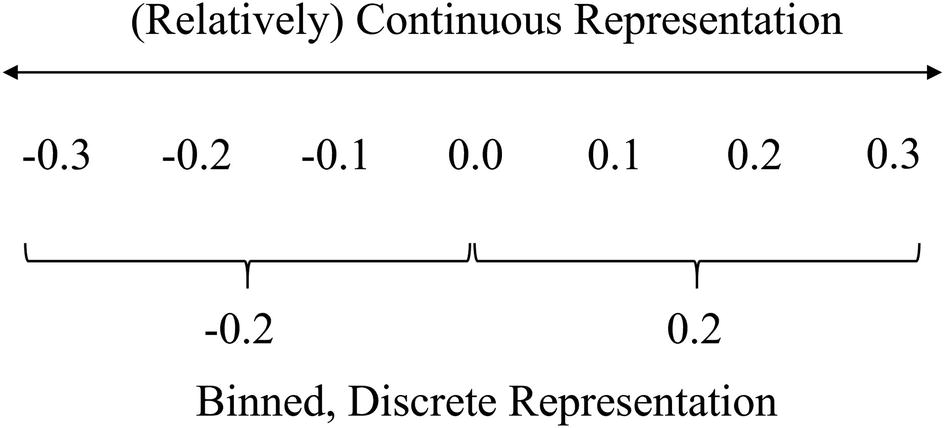
Continuous vs. binned, discrete representation
(You could view magnitude-based pruning as a selective form of quantization, in which weights smaller in magnitude than a certain threshold are “quantized to 0” and other weights are binned to themselves.)
Recall the living space analogy for pruning. Instead of outright removing certain items from your living space, imagine reducing the cost to keep each one by a little bit. You decide to downgrade your television subscription to a lower tier, decrease the electricity consumption of your light, order takeout once a week instead of twice or thrice a week, and other amends that “round” the cost of your experience down.
Post-processing quantization is a quantization procedure performed on the model after it is trained. While this method achieves a good compression rate with the advantage of decreased latency, the errors in the small approximations performed in each of the weights via quantization accumulate and lead to a significant decrease in performance.
Like the iterative approach to pruning, quantization is generally not performed on the entire network at once – this is too jarring a change, just as pruning away 95% of a network’s parameters all at once is not conducive to recovery. Rather, after a model is pretrained – ideally, pretraining develops meaningful and robust representations that can be used to help the model recover from the compression – the model undergoes Quantization Aware Training, or QAT (Figure 4-7).

Quantization Aware Training
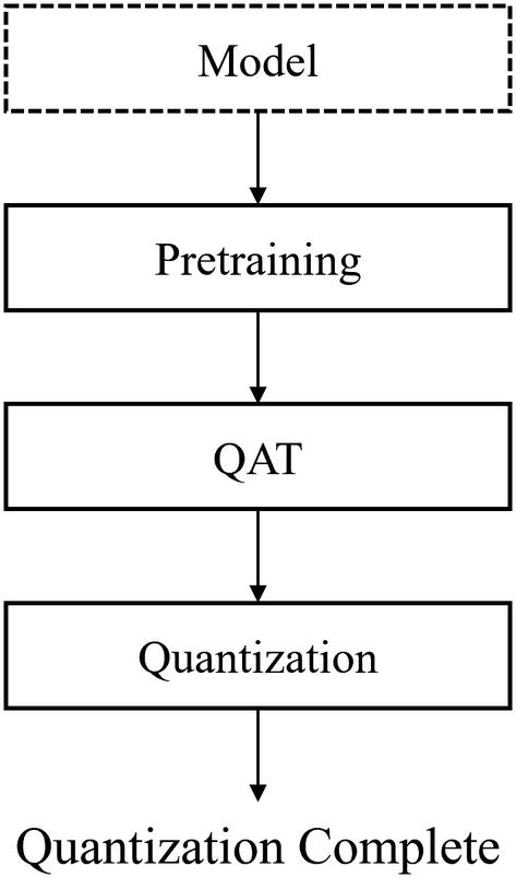
Quantization process
With quantization, a model’s storage requirements and latency can be dramatically decreased with little effect on performance.
Quantization Implementation
Like in pruning, you can quantize an entire model or quantize layers independently.
Quantizing an Entire Model
Base model for MNIST data; this will be used for applying quantization
This particular model obtains a training loss of 0.0387 and a training accuracy of 0.9918. In evaluation, it scores a loss of 0.1513 and an accuracy of 0.9720. This sort of disparity between training and testing performance indicates that some sort of compression method would be apt to apply here.
Setting up Quantization Aware Training
Performing Quantization Aware Training
Converting to TFLite model to actually quantize model
Realizing storage benefits from TFLite model
Like the pruned model, you can store the model to a file path via a variety of model saving and weight saving methods. If you load the weights by saving the entire model directly, make sure to reload the model under the scope tfmot.quantization.keras.quantize_scope.
Quantizing Individual Layers
Like in pruning, quantizing individual layers gives the advantage of specificity and hence smaller performance degradation, with the cost of a likely smaller compression than a fully quantized model.
When selecting which layers can be quantized, you can use tfmot.quantization.keras.quantize_annotate_layer, which you can wrap around a layer as you’re using it either in the Sequential or Functional API, much like prune_low_magnitude(). When quantizing individual layers, try to quantize later layers rather than the initial layers.
Quantizing individual layers by wrapping quantization annotations to individual layers while defining them
Applying quantization to the annotated layers
The quantize_apply function was not needed when quantizing the entire model using quantize_model because the quantize_model function acts as a “shortcut” that annotated and applies quantization automatically for general cases in which the “default” parameters can be applied (i.e., there is no need for customization by quantizing specific layers).
The model can then be compiled and fitted using the same training principles as discussed prior – low number of epochs, high batch size.
Defining a quantization annotation cloning function
Applying the cloning function to a (pretrained) base model
Then, apply the quantize_apply function to the annotated model and compile and fit like normal.
Weight Clustering
Weight clustering is a certainly less popular but still incredibly valuable and simple model compression method (Figure 4-9).
Weight Clustering Theory and Intuition
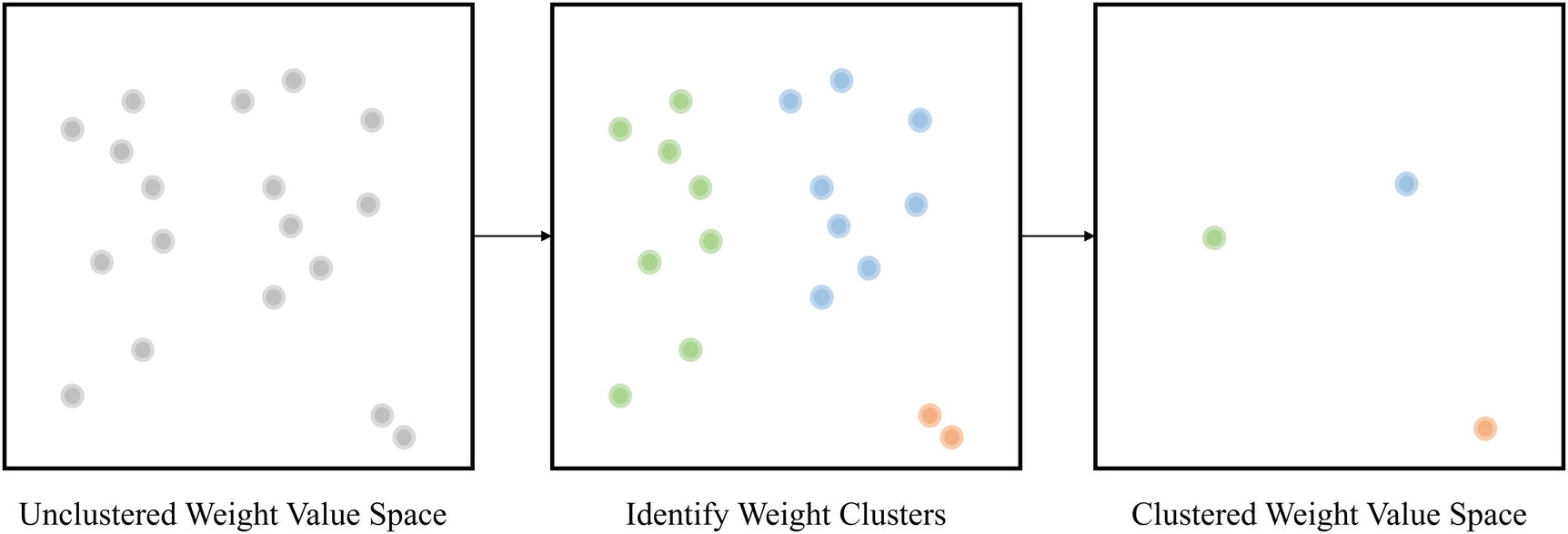
Weight clustering
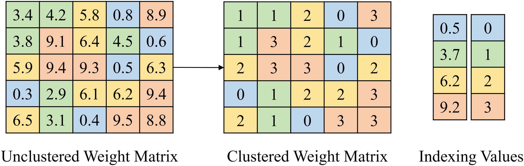
Weight clustering via indexing
The key parameter in weight clustering is determining the number of clusters. Like the percent of parameters to prune, this is a trade-off between performance and compression. If the number of clusters is very high, the change each parameter makes from its original value to the value of the centroid it was assigned is very small, allowing for more precision and easier recovery from the compression operation. However, it diminishes the compression result by increasing storage requirements both for storing the centroid values and potentially the indexes themselves. On the other hand, if the number of clusters is too small, the performance of the model may be so impaired that it cannot recover – it may simply not be possible for a model to function reasonably with a certain set of fixed parameters.
Weight Clustering Implementation
Like with pruning and quantization, you can either cluster the weights of an entire model or of individual layers.
Weight Clustering on an Entire Model
Defining clustering parameters
Creating a weight-clustered model with the specified clustering parameters
The weight-clustered model can then be compiled and fitted on the original data for fine-tuning.
Stripping clustering artifacts to realize compression benefits after fitting
After this, convert the code into a TFLite model and evaluate the size of the zipped TFLite model to see the decrease in storage size. You can also evaluate the latency of the model by using the function we defined prior in the pruning section, but make sure to re-attach an optimizer by compiling.
Like a pruned and quantized model, you can store the weight-clustered model to a file path via a variety of model saving and weight saving methods. If you load the weights by saving the entire model directly, make sure to reload the model under the scope tfmot.clustering.keras.cluster_scope.
Weight Clustering on Individual Layers
Weight clustering on individual layers follows the same syntax as pruning and quantization on individual layers, but use tfmot.clustering.keras.cluster_weights instead of tfmot.quantization.keras.quantize_apply or tfmot.sparsity.prune_low_magnitude. Like these other compression methods, you can either apply weight clustering to each layer as it is being constructed in the architecture or as a cloning function when cloning an existing model. The latter procedure of applying a compression method to individual layers is preferred because it allows for convenient pretraining and fine-tuning.
Collaborative Optimization

Relationship between model size ratio after compression and the loss in accuracy by compression method. For a certain accuracy loss, pruning + quantization is able to achieve a much smaller model size ratio after compression than pruning only or quantization only. SVD is another model compression technique that has not seen as much success as pruning and quantization
Quantization and weight clustering, or clustering preserving quantization
Quantization and pruning, or sparsity preserving quantization
Pruning and weight clustering, or sparsity preserving clustering
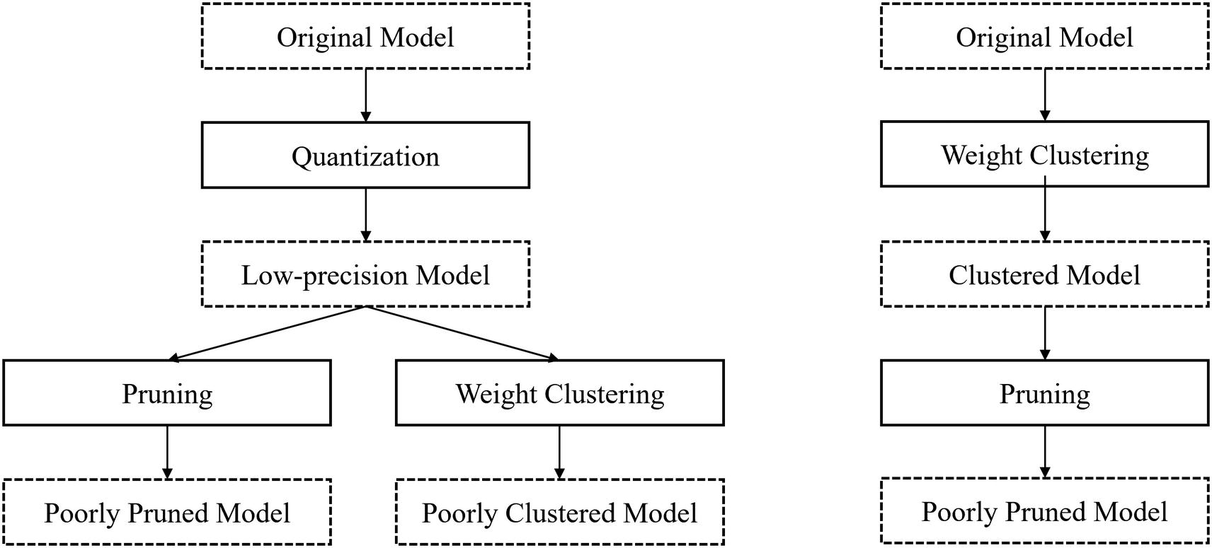
The effect of the order in which model compression methods are applied on the performance of the collaboratively optimized model. Performing quantization before pruning or weight clustering and weight clustering before pruning undermines the effect of the second compression method and therefore is an inefficient process

The undoing effect of performing weight clustering after pruning without using sparsity preserving clustering. Even though the difference in this case is small, it can be compounded significantly across each of the weight matrices for tremendous damage to the effects of pruning

The importance of model compression preservation in collaborative optimization
Sparsity Preserving Quantization
In sparsity preserving quantization , pruning is followed by quantization (Figure 4-15).
Using code and methods discussed earlier in the pruning section, obtain a pruned_model. You can use the measurement metrics defined prior to verify that the pruning procedure was successful. Use the strip_pruning function (tfmot.sparsity.keras.strip_pruning) to remove artifacts from the pruning procedure; this is necessary in order to perform quantization.
Recall that to induce Quantization Aware Training for a model, you used the quantize_model() function and then compiled and fitted the model. Performing pruning-preserving Quantization Aware Training, however, requires an additional step. The quantize_annotate_model() function is used not to actually quantize the model, but to provide annotations indicating that the entire model should be quantized. quantize_annotate_model() is used for more specific customizations of the quantization procedure, whereas quantize_model() can be thought of as the “default” quantization method. (You may similarly recall that quantize_annotate_layer() was used for another specific customization – layer-specific quantization.)

Collaborative optimization with sparsity preserving quantization
Performing sparsity preserving quantization after pruning
Cluster Preserving Quantization
In cluster preserving quantization , weight clustering is followed by quantization (Figure 4-16).
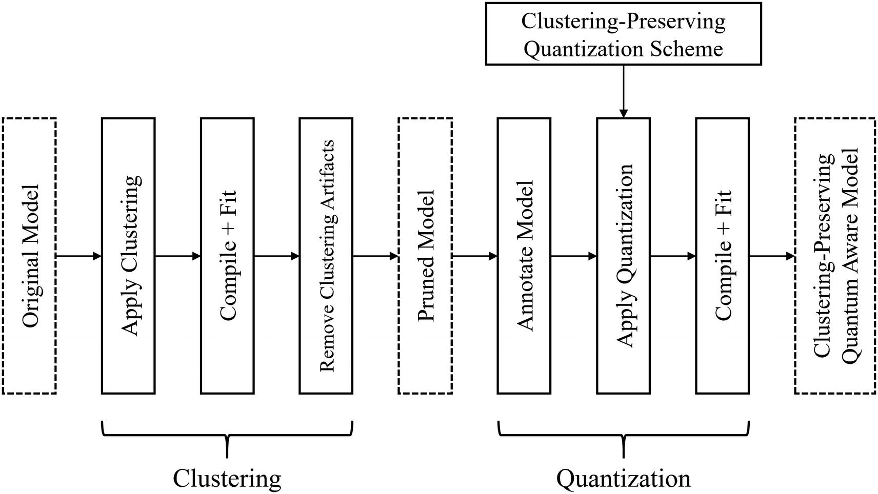
Collaborative optimization with cluster preserving quantization
Sparsity Preserving Clustering
In sparsity preserving clustering , pruning is followed by weight clustering (Figure 4-17).
Sparsity preserving clustering follows a slightly different process than cluster preserving quantization and sparsity preserving quantization.
Using code and methods discussed earlier in the pruning section, obtain a pruned_model. Strip away pruning artifacts with strip_pruning.
We need to import the cluster_weights function to perform weight clustering; prior, we imported it from tfmot.clustering.keras.cluster_weights. However, to use sparsity preserving clustering, we need to import the function from a different place: from tensorflow_model_optimization.python.core.clustering.keras.experimental.cluster import cluster_weights.
Defining clustering parameters with sparsity preservation marked
Performing sparsity preserving clustering after pruning

Collaborative optimization with sparsity preserving clustering
Case Studies
In these case studies, we will present research that has experimented with these compression methods and other variations on the presented methods to provide further concrete exploration into model compression.
Extreme Collaborative Optimization
The 2016 paper “Deep Compression: Compressing Deep Neural Networks with Pruning, Trained Quantization, and Huffman Coding”3 by Song Han, Huizi Mao, and William J. Dally was an instrumental leap forward in collaborative optimization.
- 1.
Recall that pruning is best performed as an iterative process in which connections are pruned and the network is fine-tuned on those pruned connections. In this paper, pruning reduces the model size by 9 to 13 times with no decrease in accuracy.
- 2.
Recall that weight clustering is performed by clustering weights that have similar values and setting the weights to their respective centroid values and that quantization is performed by training the model to adapt toward lower-precision weights. Weight clustering combined with quantization, after pruning, reduces the original model size by 27 to 31 times.
- 3.
Huffman coding is a compression technique that was proposed by computer scientist David A. Huffman in 1952. It allows for lossless data compression that represents more common symbols with fewer bits. Huffman coding is different from the previously discussed model compression methods because it is a post-training compression scheme; that is, there is no model fine-tuning required for the scheme to work successfully. Huffman encoding allows for even further compression – the final model is compressed with a reduction 35 to 49 times its original size.

Collaborative optimization between pruning, weight clustering, quantization, and Huffman encoding
Performance of this collaborative optimization compressed model on MNIST for LeNet and AlexNet and on ImageNet for VGG-16 model
Network | Top 1 Error | Top 5 Error | Parameters | Compression Rate |
|---|---|---|---|---|
LeNet-300-100 Compressed | 1.64% 1.58% | – | 1070 KB 27 KB | 40 times |
LeNet-5 Compressed | 0.80% 0.74% | – | 1720 KB 44 KB | 39 times |
AlexNet Compressed | 42.78% 42.78% | 19.73% 19.70% | 240 MB 6.9 MB | 35 times |
VGG-16 Compressed | 31.50% 31.17% | 11.32% 10.91% | 552 MB 11.3 MB | 49 times |
Performance of models with various compression methods applied
Rethinking Quantization for Deeper Compression
Recall that when performing quantization, Quantization Aware Training is used to orient the model toward learning weights that are robust to quantization. This is performed by simulating a quantized environment when the model is making predictions.
However, Quantization Aware Training raises a key problem: because quantization effectively “discretizes” or “bins” a functionally “continuous” weight value, the derivative with respect to the input is zero at almost everywhere, posing problems for the gradient update calculations. In order to work around this, in practice a Straight Through Estimator is used. As implied by its name, a Straight Through Estimator estimates the output gradients of the discretized layer as its input gradients without regard for the actual derivative of the actual discretized layer. A Straight Through Estimator works with relatively less aggressive quantization (i.e., the 8-bit integer quantization implemented earlier) but fails to provide sufficient estimation for more severe compressions (e.g., 4-bit integer).
To address this problem, Angela Fan and Pierre Stock, along with Benjamin Graham, Edouard Grave, Remi Gribonval, Herve Jegou, and Armand Joulin, propose quantization noise in their paper “Training with Quantization Noise for Extreme Model Compression,”4 a novel approach toward orienting a compressed model to developing quantization robust weights.

Demonstration of training without quantization noise vs. with quantization noise
Language modeling task: 16-layer transformer on WikiText-103. Image classification: EfficientNetB3 on ImageNet 1k. “Comp.” refers to “Compression.” “PPL” refers to perplexity, a metric for NLP tasks (lower is better). QAT refers to Quantization Aware Training; QN refers to quantization noise.
Quantization Method | Language Modeling | Image Classification | ||||
|---|---|---|---|---|---|---|
Size | Comp. | PPL | Size | Comp. | Top 1 | |
Uncompressed method | 942 | 1x | 18.3 | 46.7 | 1x | 81.5 |
4-bit integer quantization – Trained with QAT – Trained with QN | 118 118 118 | 8x 8x 8x | 39.4 34.1 21.8 | 5.8 5.8 5.8 | 8x 8x 8x | 45.3 59.4 67.8 |
8-bit integer quantization – Trained with QAT – Trained with QN | 236 236 236 | 4x 4x 4x | 19.6 21.0 18.7 | 11.7 11.7 11.7 | 4x 4x 4x | 80.7 80.8 80.9 |
iPQ with quantization noise compared to the performance of an uncompressed model
Quantization Method | Language Modeling | Image Classification | ||||
|---|---|---|---|---|---|---|
Size | Comp. | PPL | Size | Comp. | Top 1 | |
Uncompressed method | 942 | 1x | 18.3 | 46.7 | 1x | 81.5 |
iPQ – Trained with QAT – Trained with QN | 38 38 38 | 25x 25x 25x | 25.2 41.2 20.7 | 3.3 3.3 3.3 | 14x 14x 14x | 79.0 55.7 80.0 |
Responsible Compression: What Do Compressed Models Forget?
When we talk about compression, the two key figures we consider are the model performance and the compression factor. These two figures are often balanced and used to determine the success of a model compression operation. We often see an increase in compression accompanied by a decrease in performance – but do you wonder what types of data inputs are being sacrificed by the compression procedure? What is lying beneath the generalized performance metrics?
In “What Do Compressed Deep Neural Networks Forget?”,5 Sara Hooker, along with Aaron Courville, Gregory Clark, Yann Dauphin, and Andrea Frome, investigates just this question: how do compression methods affect what knowledge a compressed model is forced to “forget” by the compression? Hooker et al.’s findings suggest that looking merely at standard performance metrics like test set accuracy may not be enough to reveal the impact of compression on the model’s true generalization capabilities.

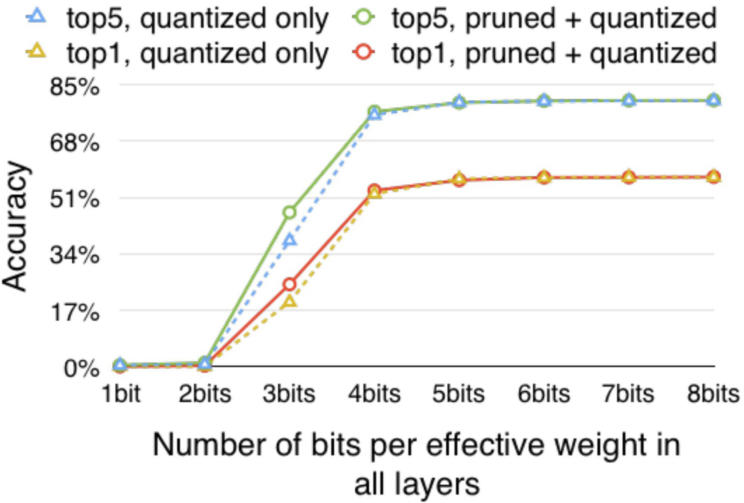
Increase or decrease in a compressed model’s recall for certain ImageNet classes. Colored bars indicate the classes in which the impact of compression is statistically significant. As a higher percent of weights are pruned, there are more classes that are statistically significantly affected by compression. Note that, interestingly, quantization suffers less from these generalization vulnerabilities than pruning does
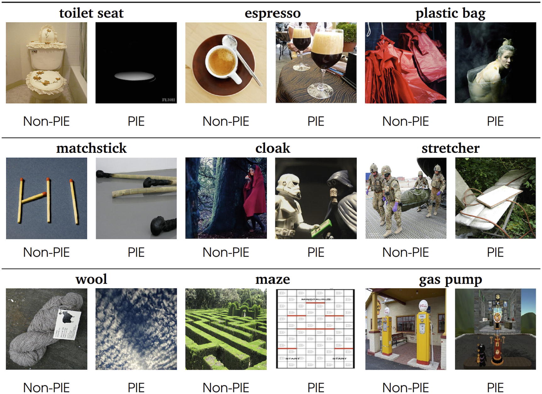
Pruning Identified Exemplars are more difficult to classify and are less represented
Compressed models, moreover, are more prone to small changes that humans would be robust to. The higher the compression, the less robust the model becomes to variations like changing brightness, contrast, blurring, zooming, and JPEG noise. This also increases the vulnerability of compressed models used in deployment to adversarial attacks, or attacks designed to subvert the model’s output by making small, cumulative changes undetectable to humans (see Chapter 2, Case Study 1, on adversarial attacks exploiting properties of transfer learning).
In addition to posing concerns for model robustness and security, these findings raise questions for the role of model compression in increasing discussion on fairness. Given that model compression disproportionately affects the model’s capacity to process less represented items in categories, model compression can amplify existing disparities in dataset representation.
Hooker et al.’s work reminds us that neural networks are complex entities that often may require more exploration and consideration than wide-reaching metrics may suggest and leaves important questions to be answered in future work on model compression.
Key Points
The goal of model compression is to decrease the “cost” a model incurs while maintaining model performance as much as possible. The “cost” of a model encompasses many factors, including storage, latency, server-side computation and power cost, and privacy. Model compression is a core element both of practical deployment and key to advancing theoretical understandings of deep learning.
In pruning, unimportant parameters or other more structured network elements are “removed” by being set to 0. This allows for much more efficient storage of the network. Pruning follows an iterative process – firstly, the importance of network elements is evaluated and the least important network elements are pruned away. Then, the model is fine-tuned on data to adapt to the pruned elements. This process repeats until the desired percentage of parameters are pruned away. A popular parameter importance criterion is by magnitude (magnitude-based pruning), in which parameters with smaller magnitudes are considered less substantial to the model’s output and set to zero.
In quantization, parameters are stored at a lower precision (usually, 8-bit integer form). This significantly decreases the storage and latency of a quantized model. However, performing post-processing quantization leads to accumulated inaccuracies that result in a large decrease in model performance. To address this, quantized models first undergo Quantization Aware Training, in which the model is in a simulated quantized environment and learns weights that are robust to quantization.
In weight clustering, weights assigned to a cluster and set to the centroid value of that cluster, such that weights similar in value to one another (i.e., part of the same cluster) make slight adjustments to be the same. This redundancy in values allows for more efficient storage. The outcome of weight clustering is heavily dependent on the number of clusters chosen.
In collaborative optimization, several model compression methods are chained together. By attaching model compression methods together, we can take advantage of each method’s unique compression strengths. However, these methods must be attached in an order and implemented with special consideration to preserve the compression effect of the previous method.
Model compression (primarily pruning) forces models to sacrifice understanding of the long tail end of the data distribution, shrinking model generalization capability. It also increases compressed models’ vulnerability to adversarial attacks and poses questions of fairness.
In the next chapter, we will discuss the automation of deep learning design with meta-optimization.