Design is as much a matter of finding problems as it is solving them.
—Bryan Lawson, Author and Architect
The previous chapter, on meta-optimization, discussed the automation of neural network design, including automated design of neural network architectures. It may seem odd to follow such a chapter on the automation of neural network architectures with a chapter on successful (implicitly, manual) neural network architecture design, but the truth is that deep learning will not reach a point anytime soon (or at all) where the state of design could possibly dismiss the need to possess an understanding of key principles and concepts in neural network architecture design. You’ve seen, firstly, that Neural Architecture Search – despite making rapid advancements – is still limited in many ways by computational accessibility and reach in the problem domain. Moreover, Neural Architecture Search algorithms themselves need to make implicit architectural design decisions to make the search space more feasible to search, which human NAS designers need to understand and encode. The design of architectures simply cannot be wholly automated away.
The success of transfer learning is earlier and stronger evidence for the proposition that the design of neural network architectures is a study that need not be studied by the average deep learning engineer. After all, if the pretrained model libraries built into TensorFlow and PyTorch don’t satisfy the needs of your problem, platforms like the TensorFlow model zoo, GitHub, and pypi host a massive quantity of easily accessible models that can be transferred, slightly adapted with minimal architectural modifications to fit the data shapes and objectives of your problem, and fine-tuned on your particular dataset.

Architectures often still need significant modifications to adapt to your particular problem domain
The process of making these more significant modifications to adapt the architecture toward success in your problem domain is a continual one; when designing your network, you should repeatedly experiment with the architecture and make architectural adaptations in response to the feedback signals of previous experiments and problems that emerge.
Both constructing successful modifications and successfully integrating them into the general model architecture require a knowledge of successful architecture-building patterns and techniques. This chapter will discuss three key ideas in neural network architecture construction – nonlinear and parallel representation, cell-based design, and network scaling. With knowledge of these concepts, you will not only be able to successfully modify general architectures but also to analytically deconstruct and understand architectures and to construct successful model architectures from scratch – a tool whose value extends not only into the construction of network architectures but cutting-edge fields like NAS.
Compartmentalization : This concept was introduced in Chapter 3 on autoencoders, in which large models were defined as a set of linked sub-models. While we will not be defining models for each component, we will need to define functions that automatically create new components of networks for us.
Automation : We will define methods of building neural networks that can build more segments of the architecture than we explicitly define in the code, allowing us to scale the network more easily and to develop complex topological patterns.
Parametrization : Networks that explicitly define key architectural parameters like the width and depth are not robust nor scalable. In order to compartmentalize and automate neural network design, we will need to define parameters relative to other parameters rather than as absolute, static values.
You’ll find that the content discussed in this chapter may feel more abstracted than that of previous chapters. This is part of the process of developing more complex architectures and a deeper feel for the dynamics of neural networks: rather than seeing an architecture as merely a collection of layers arranged in a certain format that somewhat arbitrarily and magically form a successful prediction function, you begin to identify and use motifs, residuals, parallel branches, cardinality, cells, scaling factors, and other architectural patterns and tools. This eye for design will be invaluable in the development of more professional, successful, and universal network architecture designs.
Nonlinear and Parallel Representation
The realization that purely linear neural network architecture topologies perform well but not well enough drives nonlinearity in the topology of – more or less – every successful modern neural network design. Linearity in the topology of a neural network becomes a burden when we want to scale it to obtain greater modeling power.
A good conceptual model for understanding the success and principles of nonlinear architecture topology design is to think of each layer as its own “thinker” engaged in a larger dialogue – one part of a large, connected network. Passing an input into the network is like presenting this set of thinkers with an unanswered question to consider. Each thinker sheds their unique light on the input, making some sort of transformation to it – reframing the question or adding some progress in answering it, perhaps – before passing the fruits of their consideration onto the next thinker. You want to design an arrangement of these thinkers – that is, where certain thinkers get and pass on information – such that the output of the dialogue (the answer to your input question) takes advantage of each of these thinkers’ perspectives as much as possible.
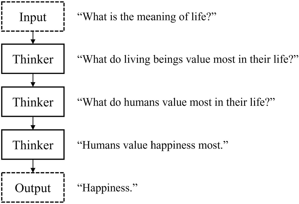
Hypothetical dialogue of a linearly arranged chain of thinkers – an answer to the age-old question, “What is the meaning of life?”
Because of the linear topology of this arrangement of thinkers, each thinker can only think through the information given to them by the previous thinker. All thinkers after the first thinker don’t have direct access to the original input question; the third thinker, for instance, is forced to answer the second thinker’s interpretation on the first thinker’s interpretation on the original question. While increasing the depth of the network can be incredibly powerful, it can also lead to this problem we see before us that later “thinkers” or layers are progressively detached from the original context of the input.

Adding a nonlinearity in the arrangement of thinkers significantly changes the output of the dialogue
In this example, the third thinker generalizes the developments of the first and second thinkers – “What do living beings value most in their life?” and “What do humans value most in their life?” – between a purely biological perspective on the value of life and another more embedded in the humanities. The third thinker responds: “Forms of reproduction – new life and ideas,” referring to the role of reproduction both in biological evolution and in the reproduction of ideas across individuals, generations, and societies of human civilization. To summarize the third thinker’s ideas, the output of the network is thus “procreation.”
With the addition of one connection from the first thinker to the third thinker, the output of the network has changed from “happiness” – a simpler, more instinctive answer – to the concept of “procreation,” a far deeper and more profound response. The key difference here is the element of merging different perspectives and ideas in consideration.
Most people would agree that more, not less, dialogue is conducive to the emergence of great ideas and insights. Similarly, think of each connection as a “one-way conversation.” When we add more connections between thinkers, we add more conversations into our network of thinkers. With sufficient number and nonlinearity connections, our network will burst into a flurry of activity, discourse, and dialogue, performing better than a linearly arranged network ever could.
Residual Connections
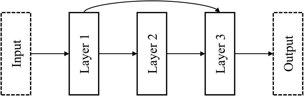
Residual connection
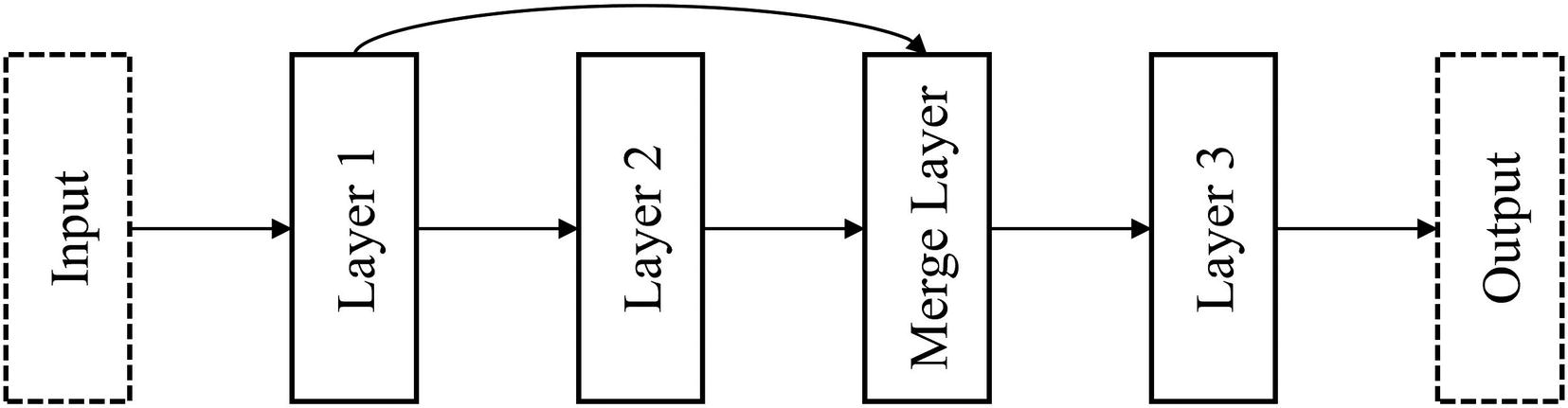
Technically correct residual connection with merge layer

ResNet-style usage of residual connections

DenseNet-style usage of residual connections
This representation of residual connections (Figure 6-4) is probably the most convenient interpretation of what a residual connection is for the purposes of implementation. It visualizes residual connections as nonlinearities added upon a “main sequence” of layers – a linear “backbone” upon which residual connections are added. In the Keras Functional API, it’s easiest to understand a residual connection as “skipping” over a “main sequence” of layers. In general, implementing nonlinearities is best performed with this concept of a linear backbone in mind, because code is written in a linear format that can be difficult to translate nonlinearities to.

Alternative interpretation of residual connection as a branching operation
Generalized nonlinearity form

Vanishing gradient problem
With residual connections, however, the backpropagation signal travels through fewer average layers to reach some particular layer’s weights for updating. This enables a stronger backpropagation signal that is better able to make use of the entire model architecture.
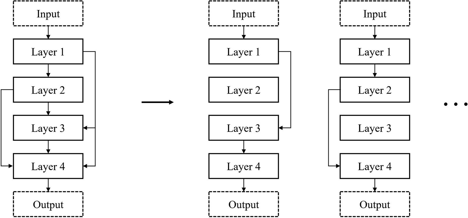
Deconstructing a DenseNet-style network into a series of linear topologies
Residual connections can also be thought of as a “failsafe” for poor performing layers. If we add a residual connection from layer A to layer C (assuming layer A is connected to layer B, which is connected to layer C), the network can “choose” to disregard layer B by learning near-zero weights for connections from A to B and from B to C while information is channeled directly from layer A to C via a residual connection. In practice, however, residual connections act more as an additional representation of the data for consideration than as failsafe mechanisms.
Creating a linear architecture using the Functional API to serve as the linear backbone for residual connections
Architecture of a sample linear backbone model
Building a residual connection by adding a merging layer

Architecture of a linear backbone with a residual connection skipping over a processing layer, dense_1
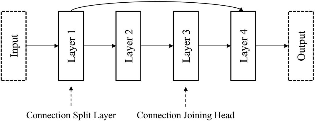
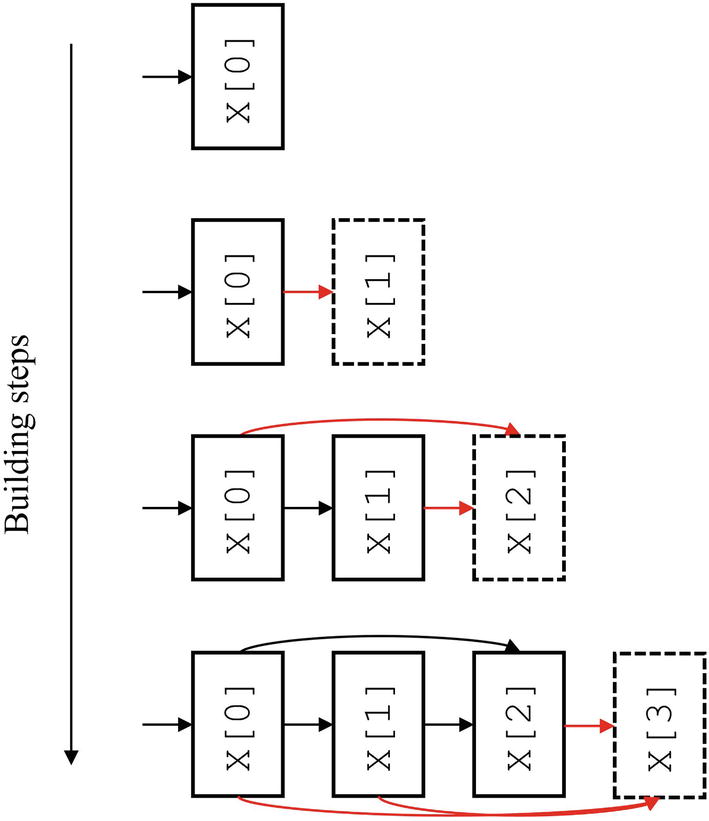
Terminology for certain layers’ relationship to one another in the automation of building residual connections
Automating the creation of a residual connection by defining a function to create a residual connection
Using the residual-connection-making function in a model architecture. (Activation functions may not be present in many listings due to space.)
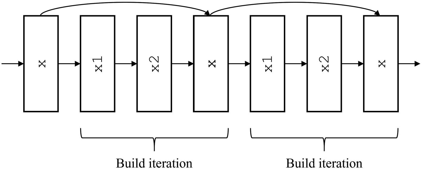
Automating the construction of residual connections by constructing in entire build iterations/blocks
It can be conceptually difficult to automate the building of these nonlinear topologies. Drawing a diagram and labeling with which template variables allows you to implement complex residual connection patterns more easily.
Building ResNet-style residual connections
Building output and aggregating ResNet-style architecture into a model

Automated ResNet-style usage of residual connections
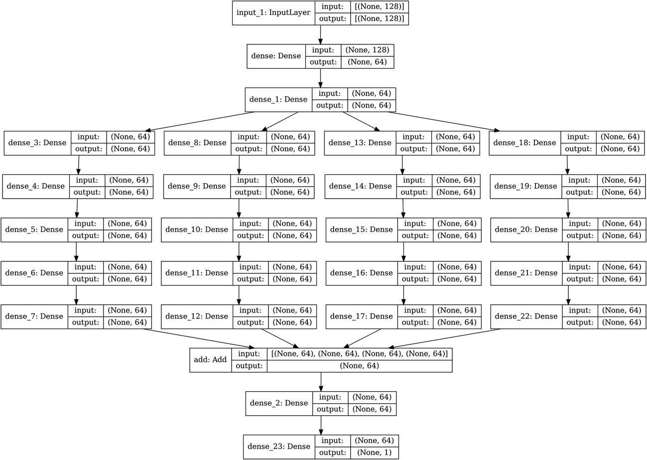
Conceptual diagram of automating the construction of DenseNet-style usage of residual connections
Adjusting the residual-connection-making function for DenseNet-style residual connections
Using the augmented residual-connection-making function to create DenseNet-style residual connections
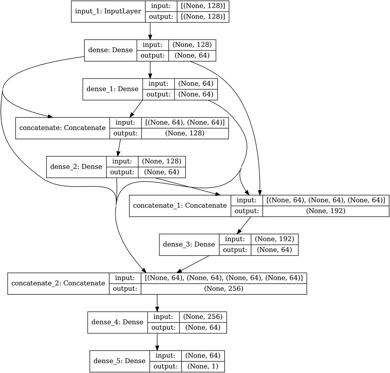
Keras visualization of DenseNet-style residual connections
This is a great example of how using predefined functions, storage, and built-in scalability in combination with one another allows for a quick and efficient building of complex topologies.
As you can see, when we begin to build more complex network designs, the Keras plotting utility starts to struggle to produce an architecture visualization that is visually consistent with our conceptual understanding of the topology. Regardless, visualization still serves as a sanity check tool to ensure that your automation of complex residual connection relationships is functioning.
Branching and Cardinality
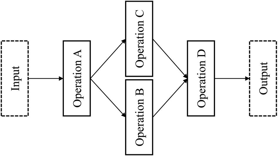
The concept of cardinality is the core framework of nonlinearity and a generalization of residual connections. While the width of a network section refers to the number of neurons in the corresponding layer(s), the cardinality of a network architecture refers to the number of “branches” (also known as parallel towers) in a nonlinear space at a certain location in a neural network architecture.

A sample component of a neural network architecture with a cardinality of two. The numbering of the layers is arbitrary
As mentioned prior in the section on residual connections, one can generalize residual connections as a simple branching mechanism with a cardinality of two, in which one branch is the series of layers the residual connection “skips over” and the other branch is the identity function.

An architectural component of a neural network that demonstrates more extreme nonlinearity (i.e., branching and merging)
It should be noted, though, that nonlinearities should not be built arbitrarily. It can be easy to get away with building complex nonlinear topologies for the sake of nonlinearity, but you should have some idea of what purpose the topology serves to enable. Likewise, a key component of the network design is not just the architecture within which layers reside but which layers and parameters are chosen to fit within the nonlinear architecture. For instance, you may allocate different branches to use different kernel sizes or to perform different operations to encourage multiplicity of representation. See the case study in the next section on cell-based design for an example on good purposeful design of more complex nonlinearities, the Inception cell.
The logic of branch representations and cardinality in architectural designs is very similar to that of residual connections. This sort of representation is the natural architectural development as a generalization of the residual connection – rather than passing the information flowing through the residual connection (i.e., doing the “skipping”) through an identity function, it can be processed separate from other components of the network.
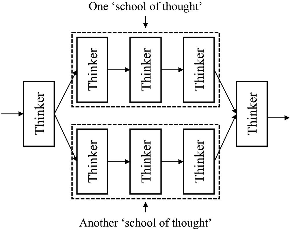
Parallel branches as conceptually organizing “thinkers” into “schools of thought”
Creating parallel branches manually

Architecture of building parallel branches
Automating the building of an individual branch
Automating the building of a series of parallel branches
Building parallel branches into a complete model architecture
Automation of building arbitrarily sized parallel branches
This sort of method is used by the ResNeXt architecture, which employs parallel branches as a generalization and “next step” from residual connections.
Case Study: U-Net
The goal of semantic segmentation is to segment, or separate, various items within an image into various classes. Semantic segmentation can be used to identify items in a picture, like cars, people, and buildings in a picture of the city. The difference between semantic segmentation and a task like image recognition is that semantic segmentation is an image-to-image task, whereas image recognition is an image-to-vector task. Image recognition tells you if an object is present in the image or not; semantic segmentation tells you where the object is located in the image by marking each pixel as part of the corresponding class or not. The output of semantic segmentation is called the segmentation map .
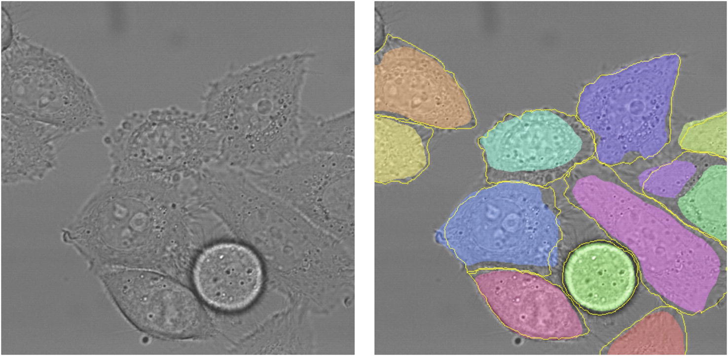
Left: input image to a segmentation model. Right: example segmentation of cells in the image. Taken from the U-Net paper by Ronneberger et al.
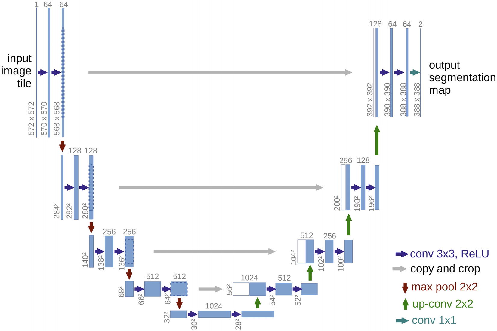
U-Net architecture. Taken from the U-Net paper by Ronneberger et al.
The left side of the architecture is termed the contracting path ; it develops successively smaller representations of the data. On the other hand, the right side is termed the expansive path , which successively increases the representation of the data. Residual connections allow the network to incorporate previously processed representations into the expansion of the representation size. This architecture allows both for localization (focus on a local region of the data input) and the use of broader context (information from farther, nonlocal regions of the image that still provide useful data).
Performance of U-Net against other segmentation models at the time on two key datasets in the ISBI cell tracking challenge 2015. Results are measured in IOU (Intersection Over Union), a segmentation metric measuring how much of the predicted and true segmented regions overlap. A higher IOU is better. U-Net beats other methods at the time by a large margin in IOU
Model | PhC-U373 Dataset | DIC-HeLa Dataset |
|---|---|---|
IMCB-SG (2014) | 0.2669 | 0.2935 |
KTH-SE (2014) | 0.7953 | 0.4607 |
HOUS-US (2014) | 0.5323 | – |
Second Best (2015) | 0.83 | 0.46 |
U-Net (2015) | 0.9203 | 0.7756 |
While the U-Net architecture is technically adaptable to all image sizes because it is built using only convolution-type layers that do not require a fixed input, the original implementation by Ronneberger et al. requires significant planning with respect to the shape of information as it passes through the network. Because the proposed U-Net architecture does not use padding, the spatial resolution is successively reduced and increased divisively (by max pooling) and additively (by convolutions). This means that residual connections must include a cropping function in order to properly merge earlier representations with later representations that have a smaller spatial size. Moreover, the input shape must be carefully planned to have a certain input size, which will not match the output.
Thus, in our implementation of the U-Net architecture, we will slightly adapt the convolutional layers to use padding such that merging and keeping track of data shapes is simpler. While implementing U-Net is relatively simple, it’s important to keep track of variables. We will name our layers with appropriate variable names such that they can be used in the make_rc() function earlier discussed to be part of a residual connection.
Building the contracting path of the U-Net architecture
Building one component of the expanding path in the U-Net architecture
Building the remaining components of the expanding path in the U-Net architecture
Adding an output layer to collapse channels and aggregating layers into a model

U-Net-style architecture implementation in Keras. Can you see the “U”?
Block/Cell Design
Recall the network of thinkers used to introduce the concept of nonlinearity. With the addition of a nonlinearity, thinkers were able to consider perspectives from multiple stages of development and processing and therefore expand their worldview to produce more insightful outputs.

Arrangement of thinkers into cells
Likewise, by arranging neural network layers into cells, we form a new unit with which we can manipulate architecturally – the cell, which contains more processing capability than a single layer. A cell can be thought of as a “mini-network.”
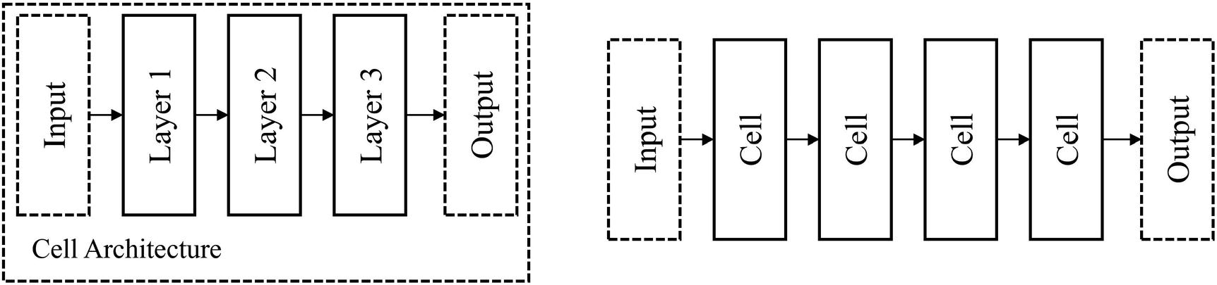
Usage of cell-based design
From a design standpoint, cells reduce the search space a neural network designer is confronted with. (You may recall that this is the justification given for a NASNet-style search space for cell architectures discussed in Chapter 5.) The designer is able to exercise fine-tuned control over the architecture of the cell, which is stacked repeatedly, therefore amplifying the effect of changes to the architecture. Contrast this with making a change to one layer in a non-cell-based network – it is unlikely that making one change would be significant enough to yield meaningfully different results (provided there exist other similar layers).
There are two key factors to consider in cell-based design: the architecture of the cell itself and the stacking method. This section will discuss methods of stacking across sequential and nonlinear cell design.
Sequential Cell Design
Sequential cell designs are – as implied by the name – cell architectures that follow a sequential, or linear, topology. While sequential cell designs have not generally performed as well as nonlinear cell designs, they can be useful as a beginning location to illustrate key concepts that will be used in nonlinear cell designs.
Building a static dense cell
Stacking static dense cells together

Visualization of cell-based design architecture

Visualization of architecture stacking convolutional and dense cells
Note that while we are building a cell-based architecture, we’re not using compartmentalized design (introduced in Chapter 3 on autoencoders). That is, while conceptually we understand that the model is built in terms of repeated block segments, we do not build that into the actual implementation of the model by defining each cell as a separate model. In this case, there is no need for compartmentalized design since we do not need to access the output of any one particular cell. Moreover, defining builder functions should serve as a sufficient code-level conceptual organization of how the network is constructed. The primary burden of using compartmentalized design with cell-based structures is the need to keep track of the input shape of the previous cell’s output in an automated fashion, which is required when defining separate models. However, implementing compartmentalized design will make Keras’ architecture visualizations more consistent with our conceptual understanding of cell-based models by visualizing cells rather than the entire sequence of layers.
Building a static convolutional cell
Stacking convolutional and dense cells together in a linear fashion
Note that static dense and static convolutional cells have different effects on the data input shapes they are applied to. Static dense cells always output the same data output shape, since the user specifies the number of nodes the input will be projected to when defining a Dense layer in Keras. On the other hand, static convolutional cells output different data output shapes, depending on which data input shapes they received. (This is discussed in more detail in Chapter 2 on transfer learning.) Because different primary layer types in cell designs can yield different impacts on the data shape, it is general convention not to build static cells.
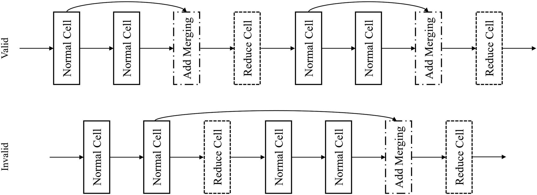
Instead, cells are generally built by their effect on the output shape, such that they can more easily be stacked together. This is especially helpful in nonlinear stacking patterns, in which cell outputs must match to be merged in a valid fashion. Generally, cells can be categorized as reduction cells or normal cells. Normal cells keep the output shape the same shape as the input shape, whereas reduction cells decrease the output shape from the input shape. Many modern architectures employ multiple designs for normal and reduction cells that are stacked repeatedly throughout the model.
Building normal and reduction cells
Stacking reduction and normal cells linearly

Architecture of alternating stacks of cells
Building convolutional normal and reduction cells is similar, but we need to keep track of three shape elements rather than one. Like in the context of autoencoders and other shape-sensitive contexts, it’s best to use padding='same' to keep the input and output shapes the same.
Building a convolutional normal cell
Building a convolutional reduction cell
These two cells can then be stacked in a linear arrangement, as previously demonstrated. Alternatively, these cells can be stacked in a nonlinear format. To do this, we’ll use the methods and ideas developed from the nonlinear and parallel representation section.

Nonlinear stacking of cells
Demonstration of residual connection usage across cells
Stacking convolutional normal and reduction cells together in nonlinear fashion with residual connections

Residual connections across normal cells
Cells can similarly be stacked in DenseNet style and with parallel branches for more complex representation. If you’re using linear cell designs, it’s recommended to use nonlinear stacking methods to add nonlinearity into the general network topology.
Nonlinear Cell Design
Nonlinear cell designs have only one input and output, but use nonlinear topologies to develop multiple parallel representations and processing mechanisms, which are combined into an output. Nonlinear cell designs are generally more successful (and hence more popular) because they allow for the construction of more powerful cells.
Building nonlinear cell designs is relatively simple with knowledge of nonlinear representation and sequential cell design. The design of nonlinear cells closely follows the previous discussion on nonlinear and parallel representation. Nonlinear cells form organized, highly efficient feature extraction modules that can be chained together to successively process information in a powerful, easily scalable manner.
Branch-based design is especially powerful in the design of nonlinear cell architectures. It is able to effectively extract and merge different parallel representations of data in one compact, stackable cell.
Build a convolutional nonlinear normal cell

Hypothetical architecture of nonlinear normal cell
Building a convolutional nonlinear reduction cell
Hypothetical architecture of a nonlinear reduction cell
These two cells (and any other additional designs for normal or reduction cells) can be stacked linearly. Because nonlinearly designed cells contain sufficient nonlinearity, there is less of a need to be aggressive in nonlinear stacking. Stacking nonlinear cells sequentially is a tried-and-true formula. One concern that could arise with linear stacking arises if you are stacking so many cells together that the depth of the network poses problems for cross-network information flow. Using residual connections across cells can help to address this problem. In the case study for this section, on the famed InceptionV3 model, we will explore a concrete example of successful nonlinear cell-based architectural design.
Case Study: InceptionV3
The famous InceptionV3 architecture , part of the Inception family of models that has become a pillar of image recognition, was proposed by Christian Szegedy, Vincent Vanhoucke, Sergey Ioffe, Jonathon Shlens, and Zbigniew Wojna in the 2015 paper “Rethinking the Inception Architecture for Computer Vision.”2 The InceptionV3 architecture, in many ways, laid out the key principles of convolutional neural network design for the following years to come. The aspect most relevant for this context is its cell-based design.

Left: original Inception cell. Right: one of the InceptionV3 cell architectures
A key architectural change in the InceptionV3 module designs is the factorization of large filter sizes like 5x5 into a combination of smaller filter sizes. For instance, the effect of a 5x5 filter can be “factored” into a series of two 3x3 filters; a 5x5 filter applied on a feature map (with no padding) yields the same output shape as two 3x3 filters: (w-4, h-4, d). Similarly, a 7x7 filter can be “factored” into three 3x3 filters. Szegedy et al. note that this factorization does not decrease representative power while promoting faster learning. This module will be termed the symmetric factorization module , although in implementation within the context of the InceptionV3 architecture it is referred to as Module A .

Factorizing n by n filters as operations of smaller filters

Expanded filter bank cell – blocks within the cell are further expanded by branching into other filter sizes
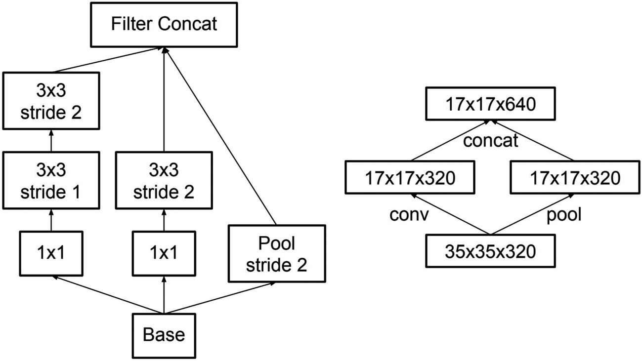
Design of a reduction cell
- 1.
A series of convolutional and pooling layers to perform initial feature extraction (these are not part of any module).
- 2.
Three repeats of the symmetric convolution module/Module A.
- 3.
Reduction module.
- 4.
Four repeats of the asymmetric convolution module/Module B.
- 5.
Reduction module.
- 6.
Two repeats of the expanded filter bank module/Module C.
- 7.
Pooling, dense layer, and softmax output.
Another often unnoticed but important feature of the Inception family of architectures is the 1x1 convolution, which is present in every Inception cell design, often as the most frequently occurring element in the architecture. As discussed in previous chapters, using convolutions with kernel size (1,1) is convenient in terms of building architectures like autoencoders when there is a need to collapse the number of channels. In terms of model performance, though, 1x1 convolutions serve a key purpose in the Inception architecture: computing cheap filter reductions before expensive, larger kernels are applied to feature map representations. For instance, suppose at some location in the architecture 256 filters are passed into a 1x1 convolutional layer; the 1x1 convolutional layer can reduce the number of filters to 64 or even 16 by learning the optional combination of values for each pixel from all 256 filters. Because the 1x1 kernel does not incorporate any spatial information (i.e., it doesn’t take into account pixels next to one another), it is cheap to compute. Moreover, it isolates the most important features for the following larger (and thus more expensive) convolution operations that incorporate spatial information.
Performance of InceptionV3 architecture against other models in ImageNet
Architecture | Top 5 Error | Top 1 Error |
|---|---|---|
GoogLeNet | – | 9.15% |
VGG | – | 7.89% |
Inception | 22% | 5.82% |
PReLU | 24.27% | 7.38% |
InceptionV3 | 18.77% | 4.2% |
Performance of an ensemble of InceptionV3 architectures compared against ensembles of other architecture models
Architecture | # Models | Top 5 Error | Top 1 Error |
|---|---|---|---|
VGGNet | 2 | 23.7% | 6.8% |
GoogLeNet | 7 | – | 6.67% |
PReLU | – | – | 4.94% |
Inception | 6 | 20.1% | 4.9% |
InceptionV3 | 4 | 17.2% | 3.58% |
The full InceptionV3 architecture is available at keras.applications.InceptionV3 with available ImageNet weights for transfer learning or just as a powerful architecture (used with random weight initialization) for image recognition and modeling.
Building a simple InceptionV3 Module A architecture
Visualization of a Keras InceptionV3 cell
Besides getting to work with large neural network architectures directly, another benefit of implementing these sorts of architectures from scratch is customizability. You can insert your own cell designs, add nonlinearities across cells (which InceptionV3 does not implement by default), or increase or decrease how many cells you stack to adjust the network depth. Moreover, cell-based structures are incredibly simple and quick to implement, so this comes at little cost.
Neural Network Scaling
Successful neural network architectures are generally not built to be static in their size. Through some mechanism, these network architectures are scalable to different sets of problems. In the previous chapter, for instance, we explored how NASNet-style Neural Architecture Search design allowed for the development of successful cell architectures that could be scaled by stacking different lengths and combinations of the discovered cells. Indeed, a large advantage to cell-based design is inherent scalability. In this section, we’ll discuss scaling principles that are applicable to all sorts of architectures – both cell-based and not.

Scaling a model to different sizes
There are generally two dimensions that can be scaled – the width (i.e., the number of nodes, filters, etc. in each layer) and length (i.e., the number of layers) in the network. These two dimensions are easily defined in linear topologies but are more ambiguous in nonlinear topologies. To make scaling simple, there are generally two paths to deal with nonlinearity. If the nonlinearity is simple enough that there is an easily identifiable linear backbone (e.g., residual connection-based architectures or simple branch architectures), the linear backbone itself is scaled. If the nonlinearity is too complex, arrange it into cells that can be linearly stacked together and scaled depth-wise. We’ll discuss these ideas more in detail.
You find that it yields insufficiently high performance on your dataset, even when trained until fruition. You suspect that the maximum predictive capacity of the model is not enough to model your dataset.
You find that the model performs fine as is, but you want to decrease its size to make it more portable in a systematic way without damaging the key attributes that contribute to the model’s performance.
You find that the model performs well as is, but you want to open-source the model for usage by the community or would like to employ it in some other context in which it will be applied to a diverse array of problem domains.
The principles of neural network scaling provide the key concepts to increase or decrease the size of your neural network in a systematic and structured fashion. After you have a candidate model architecture built, incorporating scalability into its design makes it more accessible across all sorts of problems.
Input Shape Adaptable Design
One method of scaling is to adapt the neural network to the input shape size. This is a direct method of scaling the architecture in relation to the complexity of the dataset, in which the relative resolution of the input shape is used to approximate the level of predictive power that needs to be allocated to process it adequately. Of course, it is not always true that the size of the input shape is indicative of the dataset’s complexity to model. The primary idea of input shape adaptable design is that a larger input shape indicates more complexity and therefore requires more predictive power relative to a smaller input (the opposite relationship being true as well). Thus, a successful input shape adaptable design is able to modify the network in accordance to chances in the input shape.
This sort of scaling is a practical one, given that input shape is a key vital component of using and transferring model architectures (i.e., if it is not correctly set up, the code will not run). It allows you to directly build model architectures that respond to different resolutions, sizes, vocabulary lengths, etc. with correspondingly more or less predictive resource allocation.
Adding a resizing layer with an adaptable input layer
This sort of resizing design has the benefit of portability in deployment; it’s easy to make valid predictions by passing in an image (or some other data form with appropriate code modifications) of any size into the network without any preprocessing. However, it doesn’t quite count as scaling in that computational resources are not being allocated to adapt to the input shape. If we pass an image with a very high resolution – (1024, 1024, 3), for instance – into the network, it will lose a tremendous level of information by naïvely resizing to a certain height or width.
Creating a list of widths via a recursive architectural policy
Building a model with the scalable architectural policy to determine network widths. We begin reading from the i+1th index because the first index contains the input width
This model, albeit simple, is now capable of being transferred to datasets of different input sizes.
We can similarly apply these ideas to convolutional neural networks. Note that convolutional layers can accept arbitrarily sized inputs, but nevertheless we can change the number of filters used in each layer by finding and applying generalized rules in the existing architecture to be scaled. In convolutional neural networks, we want to expand the number of filters to compensate for decreases in image resolution. Thus, the number of filters should increase over time relative to the original input shape to perform this resource compensation properly.
 , where w is the original width (the expression is purposely left in unsimplified form). Thus, a 128x128 image would begin with 8 filters, whereas a 256x256 image would begin with 16 filters. The number of filters a network has is scaled up or down relative to the size of the input image. We define the number of filters the last convolutional layer has simply to be 23 = 8 times the number of original filters.
Setting important parameters for convolutional scalable models
Architectural policy to determine the number of filters at each convolutional layer
The sequence of filters for a (128,128,3) image, according to this method, is [8, 8, 8, 16, 16, 32, 32, 32, 64, 64]. The sequence of filters for a (256,256,3) image is [16, 16, 16, 32, 32, 64, 64, 64, 128, 128]. Note that we don’t define the architectural policy in this case recursively.
By determining which segment to enter by measuring progress rather than the deterministic layer (i.e., if the current layer is past Layer 3), this script is also scalable across depth. By adjusting the num_layers parameter, you can “shrink” or “stretch” this sequence across any desired depth. Because higher resolutions generally warrant longer depths, you can also generalize the num_layers parameter as a function of the input resolution, like num_layers = round(np.log2(128)*3). Note that in this case we are using the logarithm to prevent the scaling algorithm from constructing networks with depths that are too high in response to high-resolution inputs. The list and length of filters can then be used to automatically construct a neural network architecture scaled appropriately depending on the image.
- 1.
Identify architectural patterns that can be generalizable for scaling, like the depth of the network or how the width of layers changes across the length of the network.
- 2.
Generalize the architecture pattern into an architectural policy that is scalable across the scaled dimension.
- 3.
Use the architectural policy to generate concrete elements of the network architecture in response to the input shape (or other determinants of scaling).
Adaptation to input shapes is most relevant for architectures like autoencoders, in which the input shape is a key influence throughout the architecture. We’ll combine cell-based design and knowledge of autoencoders discussed in Chapter 3 to create a scalable autoencoder whose length and filter sizes can automatically be scaled to whatever input size it is being applied to.
Encoder and decoder cells, for example, autoencoder-like structure
Defining key factors in building the scalable autoencoder-like architecture
We must consider the two key dimensions of scale: width and depth.
The number of filters in a block will be doubled if the resolution is halved, and it will be halved if the resolution is doubled. This sort of relationship ensures approximate representation equilibrium throughout the network – we do not create representation bottlenecks that are too severe, a principle of network design outlined by Szegedy et al. in the Inception architecture (see case study for section on cell-based design). Assume that this network is used for a purpose like pretraining or denoising in which bottlenecks can be built less liberally in size (in other contexts, we would want to build more severe representation bottlenecks). We can keep track of this relationship by increasing i by 1 after an encoder cell is attached and decreasing it by 1 after a decoder cell is attached.
In this example, we will build our neural network not with a certain pre-specified depth, but with whatever depth is necessary to obtain a certain bottleneck size. That is, we will continue stacking encoder blocks until the data shape is equal to (or falls below) a certain desired bottleneck size. At this point, we will stack decoder blocks to progressively increase the size of the data until it reaches its original size.
Building the encoder component of the scalable autoencoder-like architecture
Building the decoder component of the scalable autoencoder-like architecture
The complete model can be aggregated as ae = keras.models.Model(inputs=inp, outputs=x). This simple autoencoder design – using two convolutions followed by a pooling operation – has been scaled to be capable of modeling any input size resolution (as long as it is a power of 2, since pooling makes approximations that are not captured in upsampling if the side length is not cleanly divisible by the pooling factor – see Chapter 3 for more on this). Scaling a model to be adaptable to different input sizes can require more work, as we’ve seen, but it makes your model more accessible and agile in experimentation and deployment.
Parametrization of Network Dimensions
In the earlier section, we focused on scaling oriented toward a necessity-level parameter: the input shape of a model. In this section, we will discuss broad parametrization of network dimensions. Adapting the network architecture to the input shape requires us to generalize the model architecture and thus formulate implicit and explicit architectural policies that may or may not be successful. The goal here is rather to parametrize the dimensions of the network for the purposes both of adaptation to different problems and also for experimentation.
As discussed in the introduction to this chapter, seldom will one round of model building suffice for deployment. By parameterizing the dimensions of a network architecture, we are able to experiment with different scales and sizes more easily and quickly for a network to optimally fit a dataset.
The key difference between parametrizing a model for the sake of experimentation and inherent scalability and parametrizing a model to adapt to the input shape is that the factors determining parametrization are user-specified, not dependent on the input shape. Rather than programming architectural policies (e.g., the pattern with which the width of a network expands from the input shape), we use multiplying coefficients. These are parameters that the user specifies that are multiplied to the current dimensions of the network. A multiplying coefficient smaller than 1 will shrink that dimension, whereas a multiplying coefficient larger than 1 will expand that dimension.
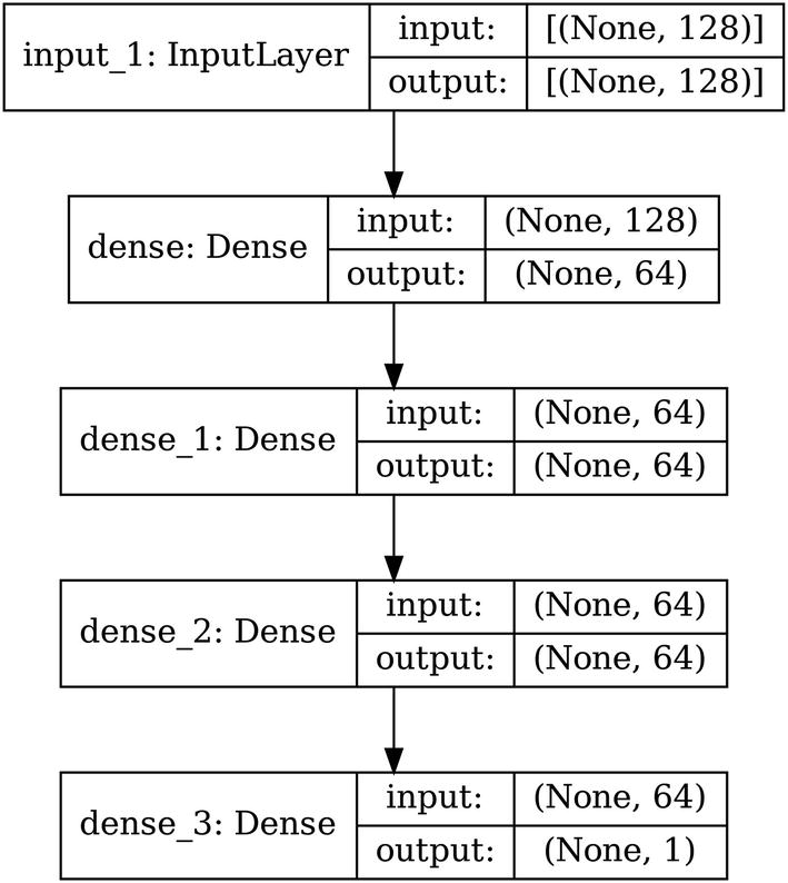
Building a simple sequential model to be parametrized
Parametrizing the width of a network
Parametrizing the depth of a network
In this case, we pass 2 into d() because 2 is the default number of layers in our model architecture. Note additionally that we are not scaling the entire depth of the network; we are leaving layers like batch normalization alone regardless of the depth coefficient, for instance. Depth-wise scaling should be applied appropriately to processing layers, not to layers like batch normalization or dropout that only shift or regularize the data flow.
The user can now adjust width_coef and depth_coef for quick experimentation and portability. The method by which you optimize the parametrization of network dimensions is up to you. One method that is likely to be successful is to use Bayesian optimization via Hyperopt or Hyperas to tune the width and depth scaling factors width_coef and depth_coef. Alternatively, one can look toward a recently growing body of research around general best practices for scaling , like the compound scaling method introduced in the successful EfficientNet architecture of models. We’ll explore this method in the case study for this section.
Parametrizing nonlinear architectures (in this case, DenseNet-style model) by relying upon a linear backbone. Complete code is not shown. Please refer to relevant DenseNet-style residual connection listing for full context
Similarly, you can parametrize the dimensions of nonlinear architectures without a nonlinear backbone that are simple, like parallel branches. If an architecture is too nonlinear to use a block-based approach toward scaling the depth dimension as introduced earlier, another method is to group these highly nonlinear topologies into blocks that can be scaled by stacking different quantities of blocks together.
By parameterizing network dimensions, you enable yourself and others to experiment and adapt the network architecture more quickly and easily, leading to improved performance on the problem.
Case Study: EfficientNet
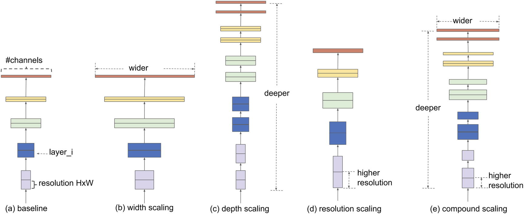
Dimensions of a neural network that can be scaled, compared with the compound scaling method
Mingxing Tan and Quoc V. Le propose the compound scaling method in their paper “EfficientNet: Rethinking Model Scaling for Convolutional Neural Networks.”3 The compound scaling method is a simple but successful scaling method in which each dimension is scaled by a constant ratio.
A set of fixed scaling constants is used to uniform scale the width, depth, and resolution used by a neural network architecture. These constants – α, β, γ – are scaled by a compound coefficient, ϕ, such that the depth is d = αϕ, the width is w = βϕ, and the resolution is r = γϕ. ϕ is defined by the user, depending on how many computational resources/predictive power they are willing to allocate toward a particular problem.
α ≥ 1, β ≥ 1, γ ≥ 1: This ensures that the constants do not decrease in value when they are raised to the power of the compound coefficient ϕ, such that a larger compound coefficient value yields in a larger depth, width, and resolution size.
α · β2 · γ2 ≈ 2: The FLOPS (floating point operations per second) of a series of convolution operations is proportional to the depth, the width squared, and the resolution squared. This is because depth operates linearly by stacking more layers, whereas the width and the resolution act upon two dimensional filter representations. To ensure computational interpretability, this constraint ensures that any value of ϕ will raise the total number of FLOPS by approximately (α · β2 · γ2)ϕ = 2ϕ.
Performance of the compound scaling method on MobileNetV1, MobileNetV2, and ResNet50 architectures
Model | FLOPS | Top 1 Acc. |
|---|---|---|
Baseline MobileNetV1 | 0.6 B | 70.6% |
Scale MobileNetV1 by width (w = 2) | 2.2 B | 74.2% |
Scale MobileNetV1 by resolution (r = 2) | 2.2 B | 74.2% |
Scale MobileNetV1 by compound scaling | 2.3 B | 75.6% |
Baseline MobileNetV2 | 0.3 B | 72.0% |
Scale MobileNetV2 by depth (d = 4) | 1.2 B | 76.8% |
Scale MobileNetV2 by width (w = 2) | 1.1 B | 76.4% |
Scale MobileNetV2 by resolution (r = 2) | 1.2 B | 74.8% |
Scale MobileNetV2 by compound scaling | 1.3 B | 77.4% |
Baseline ResNet50 | 4.1 B | 76.0% |
Scale ResNet50 by depth (d = 4) | 16.2 B | 76.0% |
Scale ResNet50 by width (w = 2) | 14.7 B | 77.7% |
Scale ResNet50 by resolution (r = 2) | 16.4 B | 77.5% |
Scale ResNet50 by compound scaling | 16.7 B | 78.8% |
Tan and Le propose explanations for the success of compound scaling that are similar to our previous intuition developed when adapting the architecture of a neural network based on the input size. By intuition, when the input image is larger, all dimensions – not just one – need to be correspondingly increased to accommodate the increase in information. Greater depth is required to process the increased layers of complexity, and greater width is needed to capture the greater quantity of information. Tan and Le’s work is novel in expressing the relationship between the network dimensions quantitatively.
Tan and Le’s paper proposes the EfficientNet family of models, which is a family of differently sized models built from the compound scaling method. There are eight models in the EfficientNet family – EfficientNetB0, EfficientNetB1, …, to EfficientNetB7, ordered from smallest to largest. The EfficientNetB0 architecture was discovered via Neural Architecture Search. In order to ensure that the derived model optimized both performance and FLOPS, the objective of the search was not merely to maximize the accuracy but to maximize a combination of performance and the FLOPS. The resulting architecture is then scaled using different values of ϕ to form the other seven EfficientNet models.
The actual open-sourced EfficientNet models are slightly adapted from their pure scaled versions. As you may imagine, compound scaling is a successful but still approximate method, as is to be expected with most scaling techniques – these are generalizations across ranges of architecture sizes. To truly maximize performance, some fine-tuning of the architecture is still needed afterward. The publicly available versions of the EfficientNet model family contain some additional architectural changes after scaling via compound scaling to further improve performance.
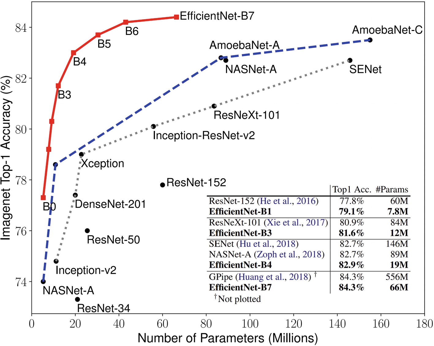
Plot of various EfficientNet models against other important model architectures in number of parameters and ImageNet top 1 accuracy
The EfficientNet model family is available in Keras applications at keras.applications.EfficientNetBx (substituting x for any number from 0 to 7). The EfficientNet implementation in Keras applications ranges from 29 MB (B0) to 256 MB (B7) in size and from 5,330,571 parameters (B0) to 66,658,687 parameters (B7). Note that the input shapes for different members of the EfficientNet family are different. EfficientNetB0 expects images of spatial dimension (224, 224); B4 expects (380, 380); B7 expects (600, 600). You can find this information in the expected input shape listed in Keras/TensorFlow applications documentation.
Looking at the EfficientNet source code in Keras is a valuable way to get a feel for how scaling is implemented on a professional level. It is available at https://github.com/keras-team/keras-applications/blob/master/keras_applications/efficientnet.py. Because this implementation is written for one of the most widely used deep learning libraries, much of the relevant code is used to generalize/parametrize the model for accessibility across various platforms and purposes. Nevertheless, its general structure of organization can be emulated for your deep learning purposes and designs.
block(), which builds a standard EfficientNet-style block given a long list of parameters, including the dropout rate, the number of incoming filters, the number of outgoing filters, etc. expand_ratio and se_ratio parameters refer to the “severity” or “intensity” of the expansion phase and the squeeze and excitation phase, which (roughly speaking) increase and decrease the representation size of the data.
EfficientNet(), which constructs an EfficientNet model given two key parameters – the width_coefficient and the depth_coefficient. Additional parameters include the dropout rate and the depth divisor (a unit used for the width of a network).
EfficientNetBx(), which simply calls the EfficientNet() architecture construction function with certain parameters appropriate to the EfficientNet structure being called. For instance, the EfficientNetB4() function returns the EfficientNet() function with a width coefficient of 1.4 and a depth coefficient of 1.8. The “unscaled” EfficientNetB0 model uses a width coefficient and depth coefficient of 1.
The key EfficientNet() function defines two functions within itself, round_filters and round_repeats, which take in the “default” number of filters and number of repeats and scale them appropriately depending on the provided width coefficient and depth coefficient.
 , where d is the depth divisor, w is the width scaling coefficient, and fo is the original number of filters. The number of new filters can never be shrunk below the value of the divisor because of the max(…) mechanism. The expression on the right simply multiplies the original number of filters by the width scaling coefficient and then applies the depth divisor to it. The depth divisor can be thought of as the bin size in quantization from Chapter 5; it is the basic unit that a parameter is scaled in terms of. The default divisor for EfficientNet is 8, meaning that the width is represented in multiples of 8. This sort of “quantization” can be easily done via the
  (integer division is performed in Python by a//d). This implementation adds
  to “balance” the scaled number of filters before “quantization”/“rounding.”
Keras EfficientNet implementation of the function used to return the scaled width of a layer
Keras EfficientNet implementation of the function used to return the scaled depth of the network
These functions are used in the building of the parametrized EfficientNet base model, allowing for easy scaling.
Key Points
There are three key concepts in efficient and advanced implementation of complex architectures – compartmentalization, automation, and parametrization.
- Nonlinear and parallel representations allow layers to pass information signals across various components of the architecture without being restricted by having to pass through many other components. This allows for the network to process information in a way that considers more perspectives and representations.
Residual connections are connections that “skip” or “jump” over other layers. ResNet-style residual connections are used repeatedly to jump over small stacks of layers. DenseNet-style residual connections, on the other hand, place residual connections between every pair of anchor points, allowing information to traverse both longer and shorter distances through the network. Residual connections are one method of addressing the vanishing gradient problem. These can be implemented quite simply through the Functional API by merging the “root” of the residual connection with the input to the “end” of the residual connection.
Branching structures and cardinality are generalizations of residual connections into broader nonlinearities. While width measures how wide one layer is (e.g., number of nodes or filters), cardinality measures how many layers wide – and therefore how many parallel representations exist and are being processed – the network is at some point.
Blocks/cell design consists of arranging layers into packaged topologies that function as cells which can be stacked upon one another to form a cell-based architecture. By arranging layers into cells and manipulating cells rather than layers, we replace the base unit of architectural construction – the layer – with a more powerful one, consisting of an agglomeration of layers. Cells can be thought of as “mini-networks” that can take on a variety of internal topologies, linear or nonlinear. In implementation, block/cell design can be implemented by constructing a function which takes in a layer to build the cell on and outputs the last layer of the cell (upon which another cell or other processing layers can be stacked).
Neural network scaling allows network architectures to be scaled for different datasets, problems, and experimentation. You can use scaling to adapt the architecture width and dimension to the input shape by identifying patterns in the neural network architecture and generalizing into an architectural policy. You can also scale architectures by parameterizing the width and the depth; these can be optimized via a method like Bayesian optimization or by a manual scaling policy like compound scaling.
In the next chapter, we will use the tools we’ve built across these multiple chapters to discuss deep learning problem-solving methods.