Chapter 3. The Architecture of Apache Flink
Chapter 2 discussed important concepts of distributed stream processing, such as parallelization, time, and state. In this chapter, we give a high-level introduction to Flink’s architecture and describe how Flink addresses the aspects of stream processing we discussed earlier. In particular, we explain Flink’s distributed architecture, show how it handles time and state in streaming applications, and discuss its fault-tolerance mechanisms. This chapter provides relevant background information to successfully implement and operate advanced streaming applications with Apache Flink. It will help you to understand Flink’s internals and to reason about the performance and behavior of streaming applications.
System Architecture
Flink is a distributed system for stateful parallel data stream processing. A Flink setup consists of multiple processes that typically run distributed across multiple machines. Common challenges that distributed systems need to address are allocation and management of compute resources in a cluster, process coordination, durable and highly available data storage, and failure recovery.
Flink does not implement all this functionality by itself. Instead, it focuses on its core function—distributed data stream processing—and leverages existing cluster infrastructure and services. Flink is well integrated with cluster resource managers, such as Apache Mesos, YARN, and Kubernetes, but can also be configured to run as a stand-alone cluster. Flink does not provide durable, distributed storage. Instead, it takes advantage of distributed filesystems like HDFS or object stores such as S3. For leader election in highly available setups, Flink depends on Apache ZooKeeper.
In this section, we describe the different components of a Flink setup and how they interact with each other to execute an application. We discuss two different styles of deploying Flink applications and the way each distributes and executes tasks. Finally, we explain how Flink’s highly available mode works.
Components of a Flink Setup
A Flink setup consists of four different components that work together to execute streaming applications. These components are a JobManager, a ResourceManager, a TaskManager, and a Dispatcher. Since Flink is implemented in Java and Scala, all components run on Java Virtual Machines (JVMs). Each component has the following responsibilities:
-
The JobManager is the master process that controls the execution of a single application—each application is controlled by a different JobManager. The JobManager receives an application for execution. The application consists of a so-called JobGraph, a logical dataflow graph (see “Introduction to Dataflow Programming”), and a JAR file that bundles all the required classes, libraries, and other resources. The JobManager converts the JobGraph into a physical dataflow graph called the ExecutionGraph, which consists of tasks that can be executed in parallel. The JobManager requests the necessary resources (TaskManager slots) to execute the tasks from the ResourceManager. Once it receives enough TaskManager slots, it distributes the tasks of the ExecutionGraph to the TaskManagers that execute them. During execution, the JobManager is responsible for all actions that require a central coordination such as the coordination of checkpoints (see “Checkpoints, Savepoints, and State Recovery”).
-
Flink features multiple ResourceManagers for different environments and resource providers such as YARN, Mesos, Kubernetes, and standalone deployments. The ResourceManager is responsible for managing TaskManager slots, Flink’s unit of processing resources. When a JobManager requests TaskManager slots, the ResourceManager instructs a TaskManager with idle slots to offer them to the JobManager. If the ResourceManager does not have enough slots to fulfill the JobManager’s request, the ResourceManager can talk to a resource provider to provision containers in which TaskManager processes are started. The ResourceManager also takes care of terminating idle TaskManagers to free compute resources.
-
TaskManagers are the worker processes of Flink. Typically, there are multiple TaskManagers running in a Flink setup. Each TaskManager provides a certain number of slots. The number of slots limits the number of tasks a TaskManager can execute. After it has been started, a TaskManager registers its slots to the ResourceManager. When instructed by the ResourceManager, the TaskManager offers one or more of its slots to a JobManager. The JobManager can then assign tasks to the slots to execute them. During execution, a TaskManager exchanges data with other TaskManagers that run tasks of the same application. The execution of tasks and the concept of slots is discussed in “Task Execution”.
-
The Dispatcher runs across job executions and provides a REST interface to submit applications for execution. Once an application is submitted for execution, it starts a JobManager and hands the application over. The REST interface enables the dispatcher to serve as an HTTP entry point to clusters that are behind a firewall. The dispatcher also runs a web dashboard to provide information about job executions. Depending on how an application is submitted for execution (discussed in “Application Deployment”), a dispatcher might not be required.
Figure 3-1 shows how Flink’s components interact with each other when an application is submitted for execution.

Figure 3-1. Application submission and component interactions
Note
Figure 3-1 is a high-level sketch to visualize the responsibilities and interactions of the components of an application. Depending on the environment (YARN, Mesos, Kubernetes, standalone cluster), some steps can be omitted or components might run in the same JVM process. For instance, in a standalone setup—a setup without a resource provider—the ResourceManager can only distribute the slots of available TaskManagers and cannot start new TaskManagers on its own. In “Deployment Modes”, we will discuss how to set up and configure Flink for different environments.
Application Deployment
Flink applications can be deployed in two different styles.
- Framework style
- In this mode, Flink applications are packaged into a JAR file and submitted by a client to a running service. The service can be a Flink Dispatcher, a Flink JobManager, or YARN’s ResourceManager. In any case, there is a service running that accepts the Flink application and ensures it is executed. If the application was submitted to a JobManager, it immediately starts to execute the application. If the application was submitted to a Dispatcher or YARN ResourceManager, it will spin up a JobManager and hand over the application, and the JobManager will start to execute the application.
- Library style
- In this mode, the Flink application is bundled in an application-specific container image, such as a Docker image. The image also includes the code to run a JobManager and ResourceManager. When a container is started from the image, it automatically launches the ResourceManager and JobManager and submits the bundled job for execution. A second, job-independent image is used to deploy TaskManager containers. A container that is started from this image automatically starts a TaskManager, which connects to the ResourceManager and registers its slots. Typically, an external resource manager such as Kubernetes takes care of starting the images and ensures that containers are restarted in case of a failure.
The framework style follows the traditional approach of submitting an application (or query) via a client to a running service. In the library style, there is no Flink service. Instead, Flink is bundled as a library together with the application in a container image. This deployment mode is common for microservices architectures. We discuss the topic of application deployment in more detail in “Running and Managing Streaming Applications”.
Task Execution
A TaskManager can execute several tasks at the same time. These tasks can be subtasks of the same operator (data parallelism), a different operator (task parallelism), or even from a different application (job parallelism). A TaskManager offers a certain number of processing slots to control the number of tasks it is able to concurrently execute. A processing slot can execute one slice of an application—one parallel task of each operator of the application. Figure 3-2 shows the relationships between TaskManagers, slots, tasks, and operators.

Figure 3-2. Operators, tasks, and processing slots
On the left-hand side of Figure 3-2 you see a JobGraph—the nonparallel representation of an application—consisting of five operators. Operators A and C are sources and operator E is a sink. Operators C and E have a parallelism of two. The other operators have a parallelism of four. Since the maximum operator parallelism is four, the application requires at least four available processing slots to be executed. Given two TaskManagers with two processing slots each, this requirement is fulfilled. The JobManager spans the JobGraph into an ExecutionGraph and assigns the tasks to the four available slots. The tasks of the operators with a parallelism of four are assigned to each slot. The two tasks of operators C and E are assigned to slots 1.1 and 2.1 and slots 1.2 and 2.2, respectively. Scheduling tasks as slices to slots has the advantage that many tasks are colocated on the TaskManager, which means they can efficiently exchange data within the the same process and without accessing the network. However, too many colocated tasks can also overload a TaskManager and result in bad performance. In “Controlling Task Scheduling” we discuss how to control the scheduling of tasks.
A TaskManager executes its tasks multithreaded in the same JVM process. Threads are more lightweight than separate processes and have lower communication costs but do not strictly isolate tasks from each other. Hence, a single misbehaving task can kill a whole TaskManager process and all tasks that run on it. By configuring only a single slot per TaskManager, you can isolate applications across TaskManagers. By leveraging thread parallelism inside a TaskManager and deploying several TaskManager processes per host, Flink offers a lot of flexibility to trade off performance and resource isolation when deploying applications. We will discuss the configuration and setup of Flink clusters in detail in Chapter 9.
Highly Available Setup
Streaming applications are typically designed to run 24/7. Hence, it is important that their execution does not stop even if an involved process fails. To recover from failures, the system first needs to restart failed processes, and second, restart the application and recover its state. In this section, you will learn how Flink restarts failed processes. Restoring the state of an application is described in “Recovery from a Consistent Checkpoint”.
TaskManager failures
As discussed before, Flink requires a sufficient number of processing slots in order to execute all tasks of an application. Given a Flink setup with four TaskManagers that provide two slots each, a streaming application can be executed with a maximum parallelism of eight. If one of the TaskManagers fails, the number of available slots drops to six. In this situation, the JobManager will ask the ResourceManager to provide more processing slots. If this is not possible—for example, because the application runs in a standalone cluster—the JobManager can not restart the application until enough slots become available. The application’s restart strategy determines how often the JobManager restarts the application and how long it waits between restart attempts.1
JobManager failures
A more challenging problem than TaskManager failures are JobManager failures. The JobManager controls the execution of a streaming application and keeps metadata about its execution, such as pointers to completed checkpoints. A streaming application cannot continue processing if the responsible JobManager process disappears. This makes the JobManager a single point of failure for applications in Flink. To overcome this problem, Flink supports a high-availability mode that migrates the responsibility and metadata for a job to another JobManager in case the original JobManager disappears.
Flink’s high-availability mode is based on Apache ZooKeeper, a system for distributed services that require coordination and consensus. Flink uses ZooKeeper for leader election and as a highly available and durable datastore. When operating in high-availability mode, the JobManager writes the JobGraph and all required metadata, such as the application’s JAR file, into a remote persistent storage system. In addition, the JobManager writes a pointer to the storage location into ZooKeeper’s datastore. During the execution of an application, the JobManager receives the state handles (storage locations) of the individual task checkpoints. Upon completion of a checkpoint—when all tasks have successfully written their state into the remote storage—the JobManager writes the state handles to the remote storage and a pointer to this location to ZooKeeper. Hence, all data that is required to recover from a JobManager failure is stored in the remote storage and ZooKeeper holds pointers to the storage locations. Figure 3-3 illustrates this design.

Figure 3-3. A highly available Flink setup
When a JobManager fails, all tasks that belong to its application are automatically cancelled. A new JobManager that takes over the work of the failed master performs the following steps:
-
It requests the storage locations from ZooKeeper to fetch the JobGraph, the JAR file, and the state handles of the last checkpoint of the application from the remote storage.
-
It requests processing slots from the ResourceManager to continue executing the application.
-
It restarts the application and resets the state of all its tasks to the last completed checkpoint.
When running an application as a library deployment in a container environment, such as Kubernetes, failed JobManager or TaskManager containers are usually automatically restarted by the container orchestration service. When running on YARN or on Mesos, Flink’s remaining processes trigger the restart of JobManager or TaskManager processes. Flink does not provide tooling to restart failed processes when running in a standalone cluster. Hence, it can be useful to run standby JobManagers and TaskManagers that can take over the work of failed processes. We will discuss the configuration of highly available Flink setups later in “Highly Available Setups”.
Data Transfer in Flink
The tasks of a running application are continuously exchanging data. The TaskManagers take care of shipping data from sending tasks to receiving tasks. The network component of a TaskManager collects records in buffers before they are shipped, i.e., records are not shipped one by one but batched into buffers. This technique is fundamental to effectively using the networking resource and achieving high throughput. The mechanism is similar to the buffering techniques used in networking or disk I/O protocols.
Note
Note that shipping records in buffers does imply that Flink’s processing model is based on microbatches.
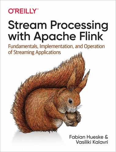
Each TaskManager has a pool of network buffers (by default 32 KB in size) to send and receive data. If the sender and receiver tasks run in separate TaskManager processes, they communicate via the network stack of the operating system. Streaming applications need to exchange data in a pipelined fashion—each pair of TaskManagers maintains a permanent TCP connection to exchange data.2 With a shuffle connection pattern, each sender task needs to be able to send data to each receiving task. A TaskManager needs one dedicated network buffer for each receiving task that any of its tasks need to send data to. Figure 3-4 shows this architecture.
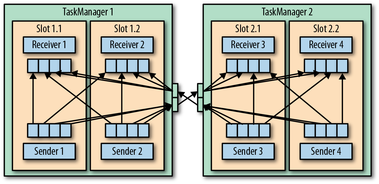
Figure 3-4. Data transfer between TaskManagers
As shown in Figure 3-4, each of the four sender tasks needs at least four network buffers to send data to each of the receiver tasks and each receiver task requires at least four buffers to receive data. Buffers that need to be sent to the other TaskManager are multiplexed over the same network connection. In order to enable a smooth pipelined data exchange, a TaskManager must be able to provide enough buffers to serve all outgoing and incoming connections concurrently. With a shuffle or broadcast connection, each sending task needs a buffer for each receiving task; the number of required buffers is quadratic to the number of tasks of the involved operators. Flink’s default configuration for network buffers is sufficient for small- to medium-sized setups. For larger setups, you need to tune the configuration as described in “Main Memory and Network Buffers”.
When a sender task and a receiver task run in the same TaskManager process, the sender task serializes the outgoing records into a byte buffer and puts the buffer into a queue once it is filled. The receiving task takes the buffer from the queue and deserializes the incoming records. Hence, data transfer between tasks that run on the same TaskManager does not cause network communication.
Flink features different techniques to reduce the communication costs between tasks. In the following sections, we briefly discuss credit-based flow control and task chaining.
Credit-Based Flow Control
Sending individual records over a network connection is inefficient and causes significant overhead. Buffering is needed to fully utilize the bandwidth of network connections. In the context of stream processing, one disadvantage of buffering is that it adds latency because records are collected in a buffer instead of being immediately shipped.
Flink implements a credit-based flow control mechanism that works as follows. A receiving task grants some credit to a sending task, the number of network buffers that are reserved to receive its data. Once a sender receives a credit notification, it ships as many buffers as it was granted and the size of its backlog—the number of network buffers that are filled and ready to be shipped. The receiver processes the shipped data with the reserved buffers and uses the sender’s backlog size to prioritize the next credit grants for all its connected senders.
Credit-based flow control reduces latency because senders can ship data as soon as the receiver has enough resources to accept it. Moreover, it is an effective mechanism to distribute network resources in the case of skewed data distributions because credit is granted based on the size of the senders’ backlog. Hence, credit-based flow control is an important building block for Flink to achieve high throughput and low latency.
Task Chaining
Flink features an optimization technique called task chaining that reduces the overhead of local communication under certain conditions. In order to satisfy the requirements for task chaining, two or more operators must be configured with the same parallelism and connected by local forward channels. The operator pipeline shown in Figure 3-5 fulfills these requirements. It consists of three operators that are all configured for a task parallelism of two and connected with local forward connections.

Figure 3-5. An operator pipeline that complies with the requirements of task chaining
Figure 3-6 depicts how the pipeline is executed with task chaining. The functions of the operators are fused into a single task that is executed by a single thread. Records that are produced by a function are separately handed over to the next function with a simple method call. Hence, there are basically no serialization and communication costs for passing records between functions.
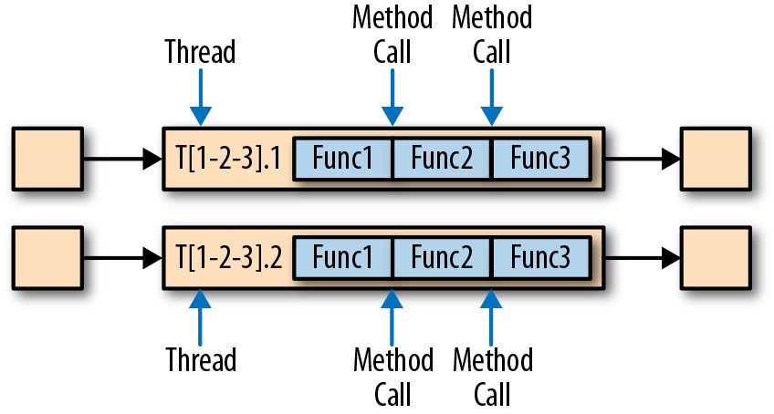
Figure 3-6. Chained task execution with fused functions in a single thread and data passing via method calls
Task chaining can significantly reduce the communication costs between local tasks, but there are also cases when it makes sense to execute a pipeline without chaining. For example, it can make sense to break a long pipeline of chained tasks or break a chain into two tasks to schedule an expensive function to different slots. Figure 3-7 shows the same pipeline executed without task chaining. All functions are evaluated by an individual task running in a dedicated thread.
Figure 3-7. Nonchained task execution with dedicated threads and data transport via buffer channels and serialization
Task chaining is enabled by default in Flink. In “Controlling Task Chaining”, we show how to disable task chaining for an application and how to control the chaining behavior of individual operators.
Event-Time Processing
In “Time Semantics”, we highlighted the importance of time semantics for stream processing applications and explained the differences between processing time and event time. While processing time is easy to understand because it is based on the local time of the processing machine, it produces somewhat arbitrary, inconsistent, and nonreproducible results. In contrast, event-time semantics yield reproducible and consistent results, which is a hard requirement for many stream processing use cases. However, event-time applications require additional configuration compared to applications with processing-time semantics. Also, the internals of a stream processor that supports event time are more involved than the internals of a system that purely operates in processing time.
Flink provides intuitive and easy-to-use primitives for common event-time processing operations but also exposes expressive APIs to implement more advanced event-time applications with custom operators. For such advanced applications, a good understanding of Flink’s internal time handling is often helpful and sometimes required. The previous chapter introduced two concepts Flink leverages to provide event-time semantics: record timestamps and watermarks. In the following, we describe how Flink internally implements and handles timestamps and watermarks to support streaming applications with event-time semantics.
Timestamps
All records that are processed by a Flink event-time streaming application must be accompanied by a timestamp. The timestamp associates a record with a specific point in time, usually the point in time at which the event that is represented by the record happened. However, applications can freely choose the meaning of the timestamps as long as the timestamps of the stream records are roughly ascending as the stream is advancing. As seen in “Time Semantics”, a certain degree of timestamp out-of-orderness is given in basically all real-world use cases.
When Flink processes a data stream in event-time mode, it evaluates time-based operators based on the timestamps of records. For example, a time-window operator assigns records to windows according to their associated timestamp. Flink encodes timestamps as 16-byte Long values and attaches them as metadata to records. Its built-in operators interpret the Long value as a Unix timestamp with millisecond precision—the number of milliseconds since 1970-01-01-00:00:00.000. However, custom operators can have their own interpretation and may, for example, adjust the precision to microseconds.
Watermarks
In addition to record timestamps, a Flink event-time application must also provide watermarks. Watermarks are used to derive the current event time at each task in an event-time application. Time-based operators use this time to trigger computations and make progress. For example, a time-window task finalizes a window computation and emits the result when the task event-time passes the window’s end boundary.
In Flink, watermarks are implemented as special records holding a timestamp as a Long value. Watermarks flow in a stream of regular records with annotated timestamps as Figure 3-8 shows.

Figure 3-8. A stream with timestamped records and watermarks
Watermarks have two basic properties:
-
They must be monotonically increasing to ensure the event-time clocks of tasks are progressing and not going backward.
-
They are related to record timestamps. A watermark with a timestamp T indicates that all subsequent records should have timestamps > T.
The second property is used to handle streams with out-of-order record timestamps, such as the records with timestamps 3 and 5 in Figure 3-8. Tasks of time-based operators collect and process records with possibly unordered timestamps and finalize a computation when their event-time clock, which is advanced by the received watermarks, indicates that no more records with relevant timestamps are expected. When a task receives a record that violates the watermark property and has smaller timestamps than a previously received watermark, it may be that the computation it belongs to has already been completed. Such records are called late records. Flink provides different ways to deal with late records, which are discussed in “Handling Late Data”.
An interesting property of watermarks is that they allow an application to control result completeness and latency. Watermarks that are very tight—close to the record timestamps—result in low processing latency because a task will only briefly wait for more records to arrive before finalizing a computation. At the same time, the result completeness might suffer because relevant records might not be included in the result and would be considered as late records. Inversely, very conservative watermarks increase processing latency but improve result completeness.
Watermark Propagation and Event Time
In this section, we discuss how operators process watermarks. Flink implements watermarks as special records that are received and emitted by operator tasks. Tasks have an internal time service that maintains timers and is activated when a watermark is received. Tasks can register timers at the timer service to perform a computation at a specific point in time in the future. For example, a window operator registers a timer for every active window, which cleans up the window’s state when the event time passes the window’s ending time.
When a task receives a watermark, the following actions take place:
-
The task updates its internal event-time clock based on the watermark’s timestamp.
-
The task’s time service identifies all timers with a time smaller than the updated event time. For each expired timer, the task invokes a callback function that can perform a computation and emit records.
-
The task emits a watermark with the updated event time.
Note
Flink restricts access to timestamps or watermarks through the DataStream API. Functions cannot read or modify record timestamps and watermarks, except for the process functions, which can read the timestamp of a currently processed record, request the current event time of the operator, and register timers.3 None of the functions exposes an API to set the timestamps of emitted records, manipulate the event-time clock of a task, or emit watermarks. Instead, time-based DataStream operator tasks configure the timestamps of emitted records to ensure they are properly aligned with the emitted watermarks. For instance, a time-window operator task attaches the end time of a window as the timestamp to all records emitted by the window computation before it emits the watermark with the timestamp that triggered the computation of the window.
Let’s now explain in more detail how a task emits watermarks and updates its event-time clock when receiving a new watermark. As you saw in “Data Parallelism and Task Parallelism”, Flink splits data streams into partitions and processes each partition in parallel by a separate operator task. Each partition is a stream of timestamped records and watermarks. Depending on how an operator is connected with its predecessor or successor operators, its tasks can receive records and watermarks from one or more input partitions and emit records and watermarks to one or more output partitions. In the following, we describe in detail how a task emits watermarks to multiple output tasks and how it advances its event-time clock from the watermarks it receives from its input tasks.
A task maintains a partition watermark for each input partition. When it receives a watermark from a partition, it updates the respective partition watermark to be the maximum of the received value and the current value. Subsequently, the task updates its event-time clock to be the minimum of all partition watermarks. If the event-time clock advances, the task processes all triggered timers and finally broadcasts its new event time to all downstream tasks by emitting a corresponding watermark to all connected output partitions.
Figure 3-9 shows how a task with four input partitions and three output partitions receives watermarks, updates its partition watermarks and event-time clock, and emits watermarks.
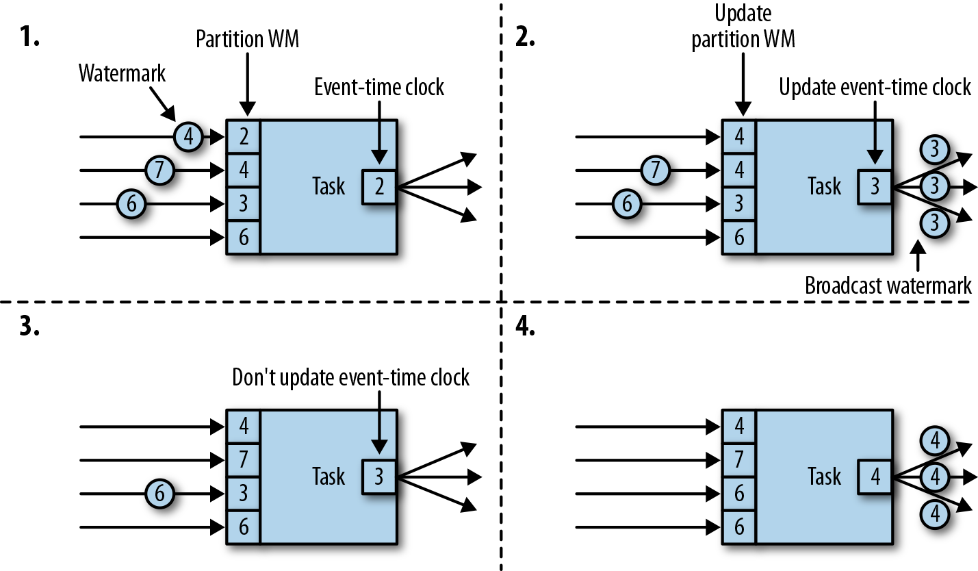
Figure 3-9. Updating the event time of a task with watermarks
The tasks of operators with two or more input streams such as Union or CoFlatMap (see “Multistream Transformations”) also compute their event-time clock as the minimum of all partition watermarks—they do not distinguish between partition watermarks of different input streams. Consequently, records of both inputs are processed based on the same event-time clock. This behavior can cause problems if the event times of the individual input streams of an application are not aligned.
Flink’s watermark-handling and propagation algorithm ensures operator tasks emit properly aligned timestamped records and watermarks. However, it relies on the fact that all partitions continuously provide increasing watermarks. As soon as one partition does not advance its watermarks or becomes completely idle and does not ship any records or watermarks, the event-time clock of a task will not advance and the timers of the task will not trigger. This situation can be problematic for time-based operators that rely on an advancing clock to perform computations and clean up their state. Consequently, the processing latencies and state size of time-based operators can significantly increase if a task does not receive new watermarks from all input tasks at regular intervals.
A similar effect appears for operators with two input streams whose watermarks significantly diverge. The event-time clocks of a task with two input streams will correspond to the watermarks of the slower stream and usually the records or intermediate results of the faster stream are buffered in state until the event-time clock allows processing them.
Timestamp Assignment and Watermark Generation
So far we have explained what timestamps and watermarks are and how they are internally handled by Flink. However, we have not yet discussed where they originate from. Timestamps and watermarks are usually assigned and generated when a stream is ingested by a streaming application. Because the choice of the timestamp is application-specific and the watermarks depend on the timestamps and characteristics of the stream, applications have to explicitly assign timestamps and generate watermarks. A Flink DataStream application can assign timestamps and generate watermarks to a stream in three ways:
-
At the source: Timestamps and watermarks can be assigned and generated by a
SourceFunctionwhen a stream is ingested into an application. A source function emits a stream of records. Records can be emitted together with an associated timestamp, and watermarks can be emitted at any point in time as special records. If a source function (temporarily) does not emit anymore watermarks, it can declare itself idle. Flink will exclude stream partitions produced by idle source functions from the watermark computation of subsequent operators. The idle mechanism of sources can be used to address the problem of not advancing watermarks as discussed earlier. Source functions are discussed in more detail in “Implementing a Custom Source Function”. -
Periodic assigner: The DataStream API provides a user-defined function called
AssignerWithPeriodicWatermarksthat extracts a timestamp from each record and is periodically queried for the current watermark. The extracted timestamps are assigned to the respective record and the queried watermarks are ingested into the stream. This function will be discussed in “Assigning Timestamps and Generating Watermarks”. -
Punctuated assigner:
AssignerWithPunctuatedWatermarksis another user-defined function that extracts a timestamp from each record. It can be used to generate watermarks that are encoded in special input records. In contrast to theAssignerWithPeriodicWatermarksfunction, this function can—but does not need to—extract a watermark from each record. We discuss this function in detail in “Assigning Timestamps and Generating Watermarks” as well.
User-defined timestamp assignment functions are usually applied as close to a source operator as possible because it can be very difficult to reason about the order of records and their timestamps after they have been processed by an operator. This is also the reason it is not a good idea to override existing timestamps and watermarks in the middle of a streaming application, although this is possible with user-defined functions.
State Management
In Chapter 2 we pointed out that most streaming applications are stateful. Many operators continuously read and update some kind of state such as records collected in a window, reading positions of an input source, or custom, application-specific operator states like machine learning models. Flink treats all states—regardless of built-in or user-defined operators—the same. In this section, we discuss the different types of states Flink supports. We explain how state is stored and maintained by state backends and how stateful applications can be scaled by redistributing state.
In general, all data maintained by a task and used to compute the results of a function belong to the state of the task. You can think of state as a local or instance variable that is accessed by a task’s business logic. Figure 3-10 shows the typical interaction between a task and its state.

Figure 3-10. A stateful stream processing task
A task receives some input data. While processing the data, the task can read and update its state and compute its result based on its input data and state. A simple example is a task that continuously counts how many records it receives. When the task receives a new record, it accesses the state to get the current count, increments the count, updates the state, and emits the new count.
The application logic to read from and write to state is often straightforward. However, efficient and reliable management of state is more challenging. This includes handling of very large states, possibly exceeding memory, and ensuring that no state is lost in case of failures. All issues related to state consistency, failure handling, and efficient storage and access are taken care of by Flink so that developers can focus on the logic of their applications.
In Flink, state is always associated with a specific operator. In order to make Flink’s runtime aware of the state of an operator, the operator needs to register its state. There are two types of state, operator state and keyed state, that are accessible from different scopes and discussed in the following sections.
Operator State
Operator state is scoped to an operator task. This means that all records processed by the same parallel task have access to the same state. Operator state cannot be accessed by another task of the same or a different operator. Figure 3-11 shows how tasks access operator state.

Figure 3-11. Tasks with operator state
Flink offers three primitives for operator state:
- List state
- Represents state as a list of entries.
- Union list state
- Represents state as a list of entries as well. But it differs from regular list state in how it is restored in the case of a failure or when an application is started from a savepoint. We discuss this difference later in this chapter.
- Broadcast state
- Designed for the special case where the state of each task of an operator is identical. This property can be leveraged during checkpoints and when rescaling an operator. Both aspects are discussed in later sections of this chapter.
Keyed State
Keyed state is maintained and accessed with respect to a key defined in the records of an operator’s input stream. Flink maintains one state instance per key value and partitions all records with the same key to the operator task that maintains the state for this key. When a task processes a record, it automatically scopes the state access to the key of the current record. Consequently, all records with the same key access the same state. Figure 3-12 shows how tasks interact with keyed state.

Figure 3-12. Tasks with keyed state
You can think of keyed state as a key-value map that is partitioned (or sharded) on the key across all parallel tasks of an operator. Flink provides different primitives for keyed state that determine the type of the value stored for each key in this distributed key-value map. We will briefly discuss the most common keyed state primitives.
- Value state
- Stores a single value of arbitrary type per key. Complex data structures can also be stored as value state.
- List state
- Stores a list of values per key. The list entries can be of arbitrary type.
- Map state
- Stores a key-value map per key. The key and value of the map can be of arbitrary type.
State primitives expose the structure of the state to Flink and enable more efficient state accesses. They are discussed further in “Declaring Keyed State at RuntimeContext”.
State Backends
A task of a stateful operator typically reads and updates its state for each incoming record. Because efficient state access is crucial to processing records with low latency, each parallel task locally maintains its state to ensure fast state accesses. How exactly the state is stored, accessed, and maintained is determined by a pluggable component that is called a state backend. A state backend is responsible for two things: local state management and checkpointing state to a remote location.
For local state management, a state backend stores all keyed states and ensures that all accesses are correctly scoped to the current key. Flink provides state backends that manage keyed state as objects stored in in-memory data structures on the JVM heap. Another state backend serializes state objects and puts them into RocksDB, which writes them to local hard disks. While the first option gives very fast state access, it is limited by the size of the memory. Accessing state stored by the RocksDB state backend is slower but its state may grow very large.
State checkpointing is important because Flink is a distributed system and state is only locally maintained. A TaskManager process (and with it, all tasks running on it) may fail at any point in time. Hence, its storage must be considered volatile. A state backend takes care of checkpointing the state of a task to a remote and persistent storage. The remote storage for checkpointing could be a distributed filesystem or a database system. State backends differ in how state is checkpointed. For instance, the RocksDB state backend supports incremental checkpoints, which can significantly reduce the checkpointing overhead for very large state sizes.
We will discuss the different state backends and their advantages and disadvantages in more detail in “Choosing a State Backend”.
Scaling Stateful Operators
A common requirement for streaming applications is to adjust the parallelism of operators due to increasing or decreasing input rates. While scaling stateless operators is trivial, changing the parallelism of stateful operators is much more challenging because their state needs to be repartitioned and assigned to more or fewer parallel tasks. Flink supports four patterns for scaling different types of state.
Operators with keyed state are scaled by repartitioning keys to fewer or more tasks. However, to improve the efficiency of the necessary state transfer between tasks, Flink does not redistribute individual keys. Instead, Flink organizes keys in so-called key groups. A key group is a partition of keys and Flink’s way of assigning keys to tasks. Figure 3-13 shows how keyed state is repartitioned in key groups.
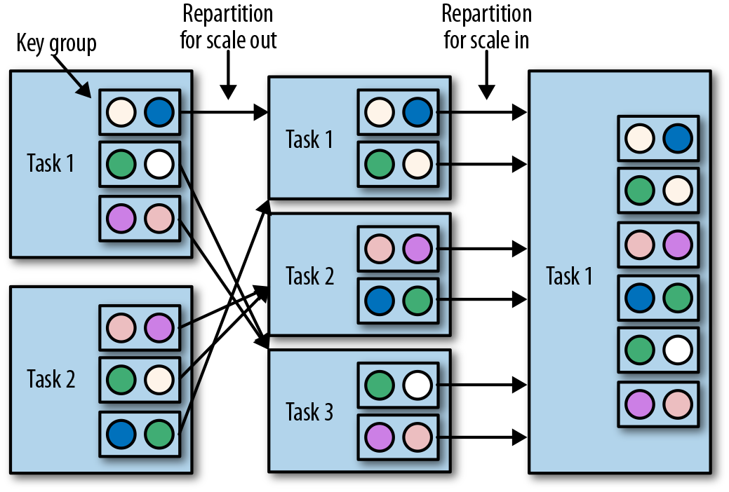
Figure 3-13. Scaling an operator with keyed state out and in
Operators with operator list state are scaled by redistributing the list entries. Conceptually, the list entries of all parallel operator tasks are collected and evenly redistributed to a smaller or larger number of tasks. If there are fewer list entries than the new parallelism of an operator, some tasks will start with empty state. Figure 3-14 shows the redistribution of operator list state.

Figure 3-14. Scaling an operator with operator list state out and in
Operators with operator union list state are scaled by broadcasting the full list of state entries to each task. The task can then choose which entries to use and which to discard. Figure 3-15 shows how operator union list state is redistributed.

Figure 3-15. Scaling an operator with operator union list state out and in
Operators with operator broadcast state are scaled up by copying the state to new tasks. This works because broadcasting state ensures that all tasks have the same state. In the case of downscaling, the surplus tasks are simply canceled since state is already replicated and will not be lost. Figure 3-16 shows the redistribution of operator broadcast state.

Figure 3-16. Scaling an operator with operator broadcast state out and in
Checkpoints, Savepoints, and State Recovery
Flink is a distributed data processing system, and as such, has to deal with failures such as killed processes, failing machines, and interrupted network connections. Since tasks maintain their state locally, Flink has to ensure that this state is not lost and remains consistent in case of a failure.
In this section, we present Flink’s checkpointing and recovery mechanism to guarantee exactly-once state consistency. We also discuss Flink’s unique savepoint feature, a “Swiss Army knife”-like tool that addresses many challenges of operating streaming applications.
Consistent Checkpoints
Flink’s recovery mechanism is based on consistent checkpoints of application state. A consistent checkpoint of a stateful streaming application is a copy of the state of each of its tasks at a point when all tasks have processed exactly the same input. This can be explained by looking at the steps of a naive algorithm that takes a consistent checkpoint of an application. The steps of this naive algorithm would be:
-
Pause the ingestion of all input streams.
-
Wait for all in-flight data to be completely processed, meaning all tasks have processed all their input data.
-
Take a checkpoint by copying the state of each task to a remote, persistent storage. The checkpoint is complete when all tasks have finished their copies.
-
Resume the ingestion of all streams.
Note that Flink does not implement this naive mechanism. We will present Flink’s more sophisticated checkpointing algorithm later in this section.
Figure 3-17 shows a consistent checkpoint of a simple application.

Figure 3-17. A consistent checkpoint of a streaming application
The application has a single source task that consumes a stream of increasing numbers—1, 2, 3, and so on. The stream of numbers is partitioned into a stream of even and odd numbers. Two tasks of a sum operator compute the running sums of all even and odd numbers. The source task stores the current offset of its input stream as state. The sum tasks persist the current sum value as state. In Figure 3-17, Flink took a checkpoint when the input offset was 5, and the sums were 6 and 9.
Recovery from a Consistent Checkpoint
During the execution of a streaming application, Flink periodically takes consistent checkpoints of the application’s state. In case of a failure, Flink uses the latest checkpoint to consistently restore the application’s state and restarts the processing. Figure 3-18 shows the recovery process.

Figure 3-18. Recovering an application from a checkpoint
An application is recovered in three steps:
-
Restart the whole application.
-
Reset the states of all stateful tasks to the latest checkpoint.
-
Resume the processing of all tasks.
This checkpointing and recovery mechanism can provide exactly-once consistency for application state, given that all operators checkpoint and restore all of their states and that all input streams are reset to the position up to which they were consumed when the checkpoint was taken. Whether a data source can reset its input stream depends on its implementation and the external system or interface from which the stream is consumed. For instance, event logs like Apache Kafka can provide records from a previous offset of the stream. In contrast, a stream consumed from a socket cannot be reset because sockets discard data once it has been consumed. Consequently, an application can only be operated under exactly-once state consistency if all input streams are consumed by resettable data sources.
After an application is restarted from a checkpoint, its internal state is exactly the same as when the checkpoint was taken. It then starts to consume and process all data that was processed between the checkpoint and the failure. Although this means Flink processes some messages twice (before and after the failure), the mechanism still achieves exactly-once state consistency because the state of all operators was reset to a point that had not seen this data yet.
We have to point out that Flink’s checkpointing and recovery mechanism only resets the internal state of a streaming application. Depending on the sink operators of an application, some result records might be emitted multiple times to downstream systems, such as an event log, a filesystem, or a database, during the recovery. For some storage systems, Flink provides sink functions that feature exactly-once output, for example, by committing emitted records on checkpoint completion. Another approach that works for many storage systems is idempotent updates. The challenges of end-to-end exactly-once applications and approaches to address them are discussed in detail in “Application Consistency Guarantees”.
Flink’s Checkpointing Algorithm
Flink’s recovery mechanism is based on consistent application checkpoints. The naive approach to taking a checkpoint from a streaming application—to pause, checkpoint, and resume the application—is not practical for applications that have even moderate latency requirements due to its “stop-the-world” behavior. Instead, Flink implements checkpointing based on the Chandy–Lamport algorithm for distributed snapshots. The algorithm does not pause the complete application but decouples checkpointing from processing, so that some tasks continue processing while others persist their state. In the following, we explain how this algorithm works.
Flink’s checkpointing algorithm uses a special type of record called a checkpoint barrier. Similar to watermarks, checkpoint barriers are injected by source operators into the regular stream of records and cannot overtake or be passed by other records. A checkpoint barrier carries a checkpoint ID to identify the checkpoint it belongs to and logically splits a stream into two parts. All state modifications due to records that precede a barrier are included in the barrier’s checkpoint and all modifications due to records that follow the barrier are included in a later checkpoint.
We use an example of a simple streaming application to explain the algorithm step by step. The application consists of two source tasks that each consume a stream of increasing numbers. The output of the source tasks is partitioned into streams of even and odd numbers. Each partition is processed by a task that computes the sum of all received numbers and forwards the updated sum to a sink. The application is depicted in Figure 3-19.

Figure 3-19. Streaming application with two stateful sources, two stateful tasks, and two stateless sinks
A checkpoint is initiated by the JobManager by sending a message with a new checkpoint ID to each data source task as shown in Figure 3-20.

Figure 3-20. JobManager initiates a checkpoint by sending a message to all sources
When a data source task receives the message, it pauses emitting records, triggers a checkpoint of its local state at the state backend, and broadcasts checkpoint barriers with the checkpoint ID via all outgoing stream partitions. The state backend notifies the task once its state checkpoint is complete and the task acknowledges the checkpoint at the JobManager. After all barriers are sent out, the source continues its regular operations. By injecting the barrier into its output stream, the source function defines the stream position on which the checkpoint is taken. Figure 3-21 shows the streaming application after both source tasks checkpointed their local state and emitted checkpoint barriers.
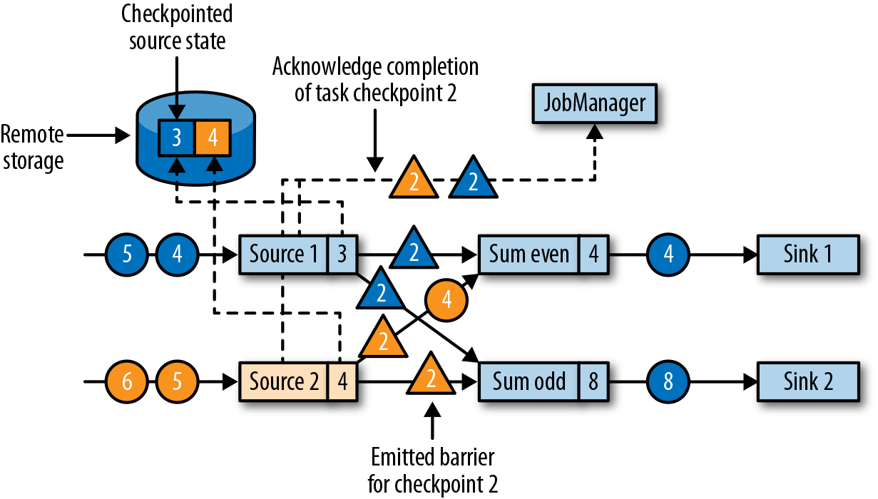
Figure 3-21. Sources checkpoint their state and emit a checkpoint barrier
The checkpoint barriers emitted by the source tasks are shipped to the connected tasks. Similar to watermarks, checkpoint barriers are broadcasted to all connected parallel tasks to ensure that each task receives a barrier from each of its input streams. When a task receives a barrier for a new checkpoint, it waits for the arrival of barriers from all its input partitions for the checkpoint. While it is waiting, it continues processing records from stream partitions that did not provide a barrier yet. Records that arrive on partitions that forwarded a barrier already cannot be processed and are buffered. The process of waiting for all barriers to arrive is called barrier alignment, and it is depicted in Figure 3-22.

Figure 3-22. Tasks wait to receive a barrier on each input partition; records from input streams for which a barrier already arrived are buffered; all other records are regularly processed
As soon as a task has received barriers from all its input partitions, it initiates a checkpoint at the state backend and broadcasts the checkpoint barrier to all of its downstream connected tasks as shown in Figure 3-23.

Figure 3-23. Tasks checkpoint their state once all barriers have been received, then they forward the checkpoint barrier
Once all checkpoint barriers have been emitted, the task starts to process the buffered records. After all buffered records have been emitted, the task continues processing its input streams. Figure 3-24 shows the application at this point.
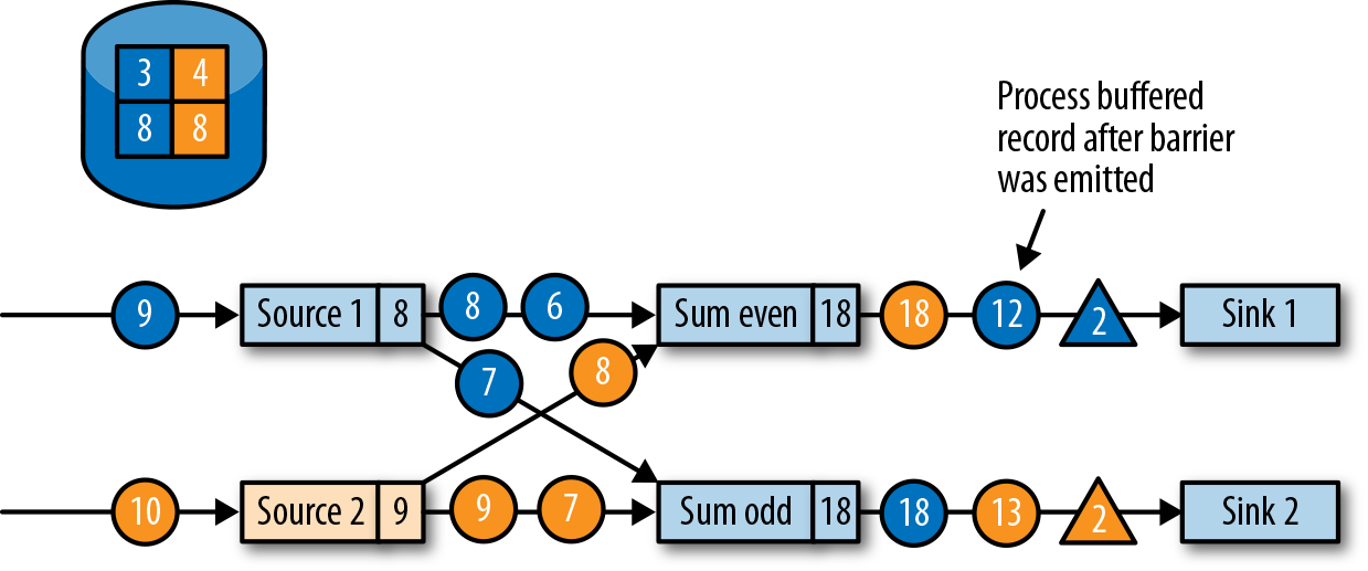
Figure 3-24. Tasks continue regular processing after the checkpoint barrier is forwarded
Eventually, the checkpoint barriers arrive at a sink task. When a sink task receives a barrier, it performs a barrier alignment, checkpoints its own state, and acknowledges the reception of the barrier to the JobManager. The JobManager records the checkpoint of an application as completed once it has received a checkpoint acknowledgement from all tasks of the application. Figure 3-25 shows the final step of the checkpointing algorithm. The completed checkpoint can be used to recover the application from a failure as described before.

Figure 3-25. Sinks acknowledge the reception of a checkpoint barrier to the JobManager and a checkpoint is complete when all tasks have acknowledged the successful checkpointing of their state
Performace Implications of Checkpointing
Flink’s checkpointing algorithm produces consistent distributed checkpoints from streaming applications without stopping the whole application. However, it can increase the processing latency of an application. Flink implements tweaks that can alleviate the performance impact under certain conditions.
While a task checkpoints its state, it is blocked and its input is buffered. Since state can become quite large and checkpointing requires writing the data over the network to a remote storage system, taking a checkpoint can easily take several seconds to minutes—much too long for latency-sensitive applications. In Flink’s design it is the responsibility of the state backend to perform a checkpoint. How exactly the state of a task is copied depends on the implementation of the state backend. For example, the FileSystem state backend and the RocksDB state backend support asynchronous checkpoints. When a checkpoint is triggered, the state backend creates a local copy of the state. When the local copy is finished, the task continues its regular processing. A background thread asynchronously copies the local snapshot to the remote storage and notifies the task once it completes the checkpoint. Asynchronous checkpointing significantly reduces the time until a task continues to process data. In addition, the RocksDB state backend also features incremental checkpointing, which reduces the amount of data to transfer.
Another technique to reduce the checkpointing algorithm’s impact on the processing latency is to tweak the barrier alignment step. For applications that require very low latency and can tolerate at-least-once state guarantees, Flink can be configured to process all arriving records during buffer alignment instead of buffering those for which the barrier has already arrived. Once all barriers for a checkpoint have arrived, the operator checkpoints the state, which might now also include modifications caused by records that would usually belong to the next checkpoint. In case of a failure, these records will be processed again, which means the checkpoint provides at-least-once instead of exactly-once consistency guarantees.
Savepoints
Flink’s recovery algorithm is based on state checkpoints. Checkpoints are periodically taken and automatically discarded according to a configurable policy. Since the purpose of checkpoints is to ensure an application can be restarted in case of a failure, they are deleted when an application is explicitly canceled.4 However, consistent snapshots of the state of an application can be used for many more things than just failure recovery.
One of Flink’s most valued and unique features are savepoints. In principle, savepoints are created using the same algorithm as checkpoints and hence are basically checkpoints with some additional metadata. Flink does not automatically take a savepoint, so a user (or external scheduler) has to explicitly trigger its creation. Flink also does not automatically clean up savepoints. Chapter 10 describes how to trigger and dispose savepoints.
Using savepoints
Given an application and a compatible savepoint, you can start the application from the savepoint. This will initialize the state of the application to the state of the savepoint and run the application from the point at which the savepoint was taken. While this behavior seems to be exactly the same as recovering an application from a failure using a checkpoint, failure recovery is actually just a special case. It starts the same application with the same configuration on the same cluster. Starting an application from a savepoint allows you to do much more.
-
You can start a different but compatible application from a savepoint. Hence, you can fix bugs in your application logic and reprocess as many events as your streaming source can provide in order to repair your results. Modified applications can also be used to run A/B tests or what-if scenarios with different business logic. Note that the application and the savepoint must be compatible—the application must be able to load the state of the savepoint.
-
You can start the same application with a different parallelism and scale the application out or in.
-
You can start the same application on a different cluster. This allows you to migrate an application to a newer Flink version or to a different cluster or data-center.
-
You can use a savepoint to pause an application and resume it later. This gives the possibility to release cluster resources for higher-priority applications or when input data is not continuously produced.
-
You can also just take a savepoint to version and archive the state of an application.
Since savepoints are such a powerful feature, many users periodically create savepoints to be able to go back in time. One of the most interesting applications of savepoints we have seen in the wild is continuously migrating a streaming application to the datacenter that provides the lowest instance prices.
Starting an application from a savepoint
All of the previously mentioned use cases for savepoints follow the same pattern. First, a savepoint of a running application is taken and then it is used to restore the state in a starting application. In this section, we describe how Flink initializes the state of an application started from a savepoint.
An application consists of multiple operators. Each operator can define one or more keyed and operator states. Operators are executed in parallel by one or more operator tasks. Hence, a typical application consists of multiple states that are distributed across multiple operator tasks that can run on different TaskManager processes.
Figure 3-26 shows an application with three operators, each running with two tasks. One operator (OP-1) has a single operator state (OS-1) and another operator (OP-2) has two keyed states (KS-1 and KS-2). When a savepoint is taken, the states of all tasks are copied to a persistent storage location.

Figure 3-26. Taking a savepoint from an application and restoring an application from a savepoint
The state copies in the savepoint are organized by an operator identifier and a state name. The operator identifier and state name are required to be able to map the state data of a savepoint to the states of the operators of a starting application. When an application is started from a savepoint, Flink redistributes the savepoint data to the tasks of the corresponding operators.
Note
Note that the savepoint does not contain information about operator tasks. That is because the number of tasks might change when an application is started with different parallelism. We discussed Flink’s strategies to scale stateful operators earlier in this section.
If a modified application is started from a savepoint, a state in the savepoint can only be mapped to the application if it contains an operator with a corresponding identifier and state name. By default, Flink assigns unique operator identifiers. However, the identifier of an operator is deterministically generated based on the identifiers of its preceding operators. Hence, the identifier of an operator changes when one of its predecessors changes, for example, when an operator is added or removed. As a consequence, an application with default operator identifiers is very limited in how it can be evolved without losing state. Therefore, we strongly recommend manually assigning unique identifiers to operators and not relying on Flink’s default assignment. We describe how to assign operator identifiers in detail in “Specifying Unique Operator Identifiers”.
Summary
In this chapter we discussed Flink’s high-level architecture and the internals of its networking stack, event-time processing mode, state management, and failure recovery mechanism. This information will come in handy when designing advanced streaming applications, setting up and configuring clusters, and operating streaming applications as well as reasoning about their performance.
1 Restart strategies are discussed in more detail in Chapter 10.
2 Batch applications can—in addition to pipelined communication—exchange data by collecting outgoing data at the sender. Once the sender task completes, the data is sent as a batch over a temporary TCP connection to the receiver.
3 Process functions are discussed in more detail in Chapter 6.
4 It is also possible to configure an application to retain its last checkpoint when it is canceled.