Chapter 11
Applications, Training, Results
There is nothing so powerful as truth—and often nothing so strange.
—Daniel Webster
Overview
This chapter walks through the process of training a test application, using an interactive training scenario to provide insight into genome metric comparisons, and scoring results. The process of genome selection, strand building, genome compare testing, metric selection, metric scoring, and reinforcement learning are outlined at a high level. This chapter does not provide a complete working application as source code, but instead explores low-level details using VGM command line tools to develop intuition about VGM internals.
The key section in this chapter for understanding metrics and scoring for the genome compare tests is “Selected Uniform Baseline Test Metrics” in the “Test Genomes and Correspondence Results” section, where a uniform baseline set of thousands of color, shape, and texture metrics are explained, as used for all genome compare tests. By examining the detailed test results in the scoring tables for each genome compare, insight is developed for metric selection, qualifier metrics tuning, classifier design, and the various learning methods discussed in Chapter 4.
This chapter illustrates how each reference genome is a separate ground truth, requiring specific metrics discovered via reinforcement learning, as discussed in Chapter 4. The volume learning model leverages reinforcement learning, beginning from the autolearning hull thresholds, to establish an independent classifier for each metric in each space for each genome. VGM allows for classifier learning by discovering optimal sets of metrics to combine and tune as a group into a structured classifier for each genome.
The VGM command line tools are used to illustrate an interactive test application development process, including genome selection and training (see Chapter 5 for tool details). Problems and work-arounds are explored. The test application is designed to locate a squirrel in a 12MB test image (see Figure 11.1). Reinforcement learning considerations are highlighted for a few robustness criteria such as rotation and lighting invariance. Detailed metric correspondence results are provided.
In addition to the test application, three unit tests are presented and executed to show how pairs of genomes compare against human expectations. The three unit test categories are (1) genome pairs which look like matches, (2) genome pairs which appear to be close matches and might spoof the metrics comparisons, and (3) genomes which are clearly nonmatches. Summary test tables are provided containing the final unit test scores, which reveal anomalies in how humans compare genomes, why ground truth data selection is critical, and why reinforcement learning and metrics tuning are needed to build a good set of baseline metrics for scoring within a suitable classifier structure.
Major topics covered in this chapter include:
–Test application outline
–Background segmentations, problems, and work-arounds
–Genome selection, strands, and training
–Baseline genome metrics selection from CSV agents
–Structured classification
–Testing and reinforcement learning
–Nine selected test genomes to illustrate genome compare metrics
–Selected metrics (Color, Texture, Shape)
–Scoring strategies
–Unit tests showing first order metrics for MATCH, NOMATCH CLOSE MATCH
–Sample high level agent code

Test Application Outline
The test image in Figure 11.1 (left) includes several views of a squirrel, with different pre-processing applied to each squirrel, so the squirrels are all slightly different. A set of test genomes are extracted from the test image for genome comparisons, identified later in this chapter. VGM operates on full resolution images, and no downsampling of images is required, so all pixel detail is captured in the model.
Here is an outline and discussion of the test application parameters, with some comparison of VGM training to DNN training:
–Image resolution: 4000x3000 (12MP image). Note that the VGM is designed to fully support common image sizes such as 5MP and 12MP, or larger. Note that a DNN pipeline operates typically on a fixed size such as 300x300 pixel images; therefore, this test application could not be performed using a DNN (see the Figure 11.1 caption).
–Robustness criteria: scale, rotation, occlusion, contrast, and lighting variations are illustrated in the compare metrics. The training set contains several identical squirrels, except that the separate squirrel instances are each modified using image pre-processing applied to change rotation, scale, and lighting to test invariance criteria. DNN training protocols add training images expressing the desired invariance criteria.
–Interactive training: interactive training sessions are explained, where the trainer selects the specific squirrel genome features to compose into a strand object, similar to the way a person would learn from an expert. (Note that an agent can also select genomes and build strands, with no intervention.) By contrast, DNN training protocols learn the entire image presented, learning both intended and unintended features, which contributes to DNN model brittleness.
–Rapid training: VGM can be trained quickly and interactively from selected features in a single image, and fine-tuned during training using additional test images or other images. VGM training is unlike DNN training, since DNN training requires epochs of training iterations (perhaps billions) as well as a costly-to-assemble set of perhaps tens and hundreds of thousands of hand-selected (or machine-selected and then hand-selected) training images of varying usefulness.
–CSV agent reinforcement learning: the best metric comparison scores for each genome comparison are learned and stored in correspondence signature vectors (CSVs) by CSV agents, using the autolearning hull thresholds yielding first order metric comparisons. Reinforcement learning and training is then applied to optimize the metrics.
Here are the key topics in the learning process covered in subsequent sections of this chapter:
–Strands and genome segmentations: selecting genomes to build strands, problems, and work-arounds
–Testing and interactive reinforcement learning: CSV agents, finding the best metrics, classifier design, metrics tuning
–Test genomes and correspondence results: compare test genomes; evaluate genome comparisons using baseline metrics
Strands and Genome Segmentations
As shown in Figure 11.2, note that the parvo segmentations (left) are intended to be smaller and more uniform in size, simulating the AR saccadic size, and the magno segmentations (right) are intended to include much larger segmentated regions as well as blockier segmentation boundaries. The jSLIC segmentation produced 1,418 total parvo scale genome regions, but only 1,246 were kept in the model, since 172 were culled because they were smaller than the AR size. See Chapter 2 regarding saccadic dithering and segmentation details. The morpho segmentation produced 551 magno scale features; 9 were culled as too large (> 640x480 pixels) and 75 were culled as smaller than the AR, yielding 467 modeled genome features. By using both the parvo and magno scale features, extra invariance is incorporated into the model. Using several additional segmentations combined would be richer and beneficial, but for brevity only two are used.

Resulting genome segmentations of the squirrel are shown in Figure 11.3. Note that the parvo features are generally smaller and more uniform in size, and the magno features contain larger and nonuniform sizes, which is one purpose for keeping both types of features. No segmentation is optimal. Comparing nonuniform sized regions (i.e. a small region compared to a large region) is performed in the MCC classifiers by normalizing each metric to the region size prior to comparison. However, based on current test results, a few metric comparisons seem to work a little better when the region size is about the same; however, region size sensitivity is generally not an issue.

Building Strands
An interactive training process is performed using the vgv command line tool discussed in Chapter 5, which displays the test image and allows for various interactive training options. Using vgv, a parvo strand and a magno strand are built to define the squirrel features, as well as define additional test features. To learn the best features, a default CSV agent is used to create and record comparison metrics in a CSV signature vector to allow the trainer to interactively learn preferred metrics. Not shown is the process of using the master learning controller, discussed in Chapter 5, to locate the best metrics and auto-generate C++ code to implement the CSV agent learnings in a custom agent.
For this example, we build a parvo strand as shown in Figure 11.4 and a magno strand as shown in Figure 11.5 to illustrate segmentation differences. By using both a parvo strand and a magno strand of the same object, robustness can be increased. Note that the magno strand includes coarser level features since the morpho segmentation is based on the 5:1 reduced resolution magno images, compared to the full resolution parvo images. Recall from Chapter 2 that the VGM models the magno pathway as the fast 5:1 subsampled low-resolution luma motion tracking channel, and the parvo channel is the slower responding high-resolution channel for RGB color using saccadic dithering for fine detail.
The following sections build strands from finer parvo features and coarser magno features, with some discussion about each strand. Note that during training, there can be problems building strands which manifest as shown in our examples. We discuss problems and work-arounds after both strands are built.
Parvo Strand Example

The commands used to build the parvo strands in Figure 11.4 are shown below. Details on the command vgv CREATE_STRAND are provided in Chapter 5.

Magno Strand Example

The commands used to build and show the magno strand in Figure 11.5 are shown below. Details on the command vgv CREATE_STRAND are provided in Chapter 5.

The magno strand in Figure 11.5 only contains three genomes, each coarser in size and shape compared to the nine finer grained genomes for the parvo strand in Figure 11.4. Also note that the squirrel back genome in Figure 11.5 contains part of the stucco wall—not good. A better strand will need to be built from a different segmentation. See the next section for discussion.
Discussion on Segmentation Problems and Work-arounds
Figure 11.5 illustrates the types of problems that can occur with image segmentation, which manifest as ill-defined genome region boundaries including wrong colors and textures, resulting in anomalous metrics and suboptimal genome region correspondence. As shown in Figure 11.5, the magno squirrel back+front_leg region is segmented incorrectly to include part of the stucco wall. What to do? Some discussion and work-arounds are given here to deal with segmentation issues as follows:
- Use a different LGN input image segmentation (raw, sharp, retinex, blur, histeq) or different color space component (Leveled, HLS_S, . . .)
- Use a different segmentation method or parma (jSLIC, morpho, . . .)
- Use multiple segmentations and perhaps create multiple strands; do not rely on a single segmentation
- Combinations of all of the above; learn and infer during training.
Future VGM releases will enhance the LGN model to provide as many of the above work-around options as possible to improve segmentation learning. The current VGM eye/LGN segmentation pipeline is still primitive but emulates how humans scan a scene by iterating around the scene, changing LGN image pre-processing parameters and resegmenting the scene in real-time. So for purposes of LGN emulation, it is advantageous to use more than one LGN image pre-processing method and more than one segmentation method, based on the analysis of the image metrics, to emulate the human visual system. Then strands can be built from the optimal segmentations.
Strand Alternatives: Single-image vs. Multi-image
There are two basic types of strands: single image or multi image. A default single-image strand collects genomes from a single-image segmentation, and a multi-image strand includes genomes from multiple-image segmentations, which may be desirable for some applications. Since the interactive training vgv app works on a single image at a time, we use single-images strands here. However, it is also possible to collect a set of independent genomes, and the agent can perform genome-by-genome correspondence and manage the scoring results.
For the current test exercise, we emulate agent-managed strands for genome-by-genome comparison, rather than using the strand set structure and shape correspondence functions provided in the VGM, since the aim is to provide more insight into the correspondence process. The strand correspondence functions are discussed in Chapter 8.
Testing and Interactive Reinforcement Learning
In this section we provide metrics comparison results between selected genome reference/target pairs in Figure 11.7 below. For each reference genome we illustrate the process of collecting and sorting genome-by-genome correspondence results to emulate the strand convenience function match__strand_set_metrics ( ... ) discussed in Chapter 8. By showing the metrics for selected genome compares, low-level details and intuition about genome correspondence is presented. For brevity, we ignore the strand metrics for angle, ellipse shape, and Fourier descriptor, which are provided in the MCC shape analysis function match__strand_shape_metrics ( ... ), and instead focus on just the set metrics and correspondence scores.
Hierarchical Parallel Ensemble Classifier
For these tests, a structured classifier is constructed, as shown in Figure 11.6, using a hierarchical ensemble of parallel MCCs. to compute correspondence using a group of CSV agents operating in an ensemble, where each CSV agent calls several MCC classifiers and performs heuristics and weighting based on the MATCH_CRITERIA and the OVERRIDES parameters (as discussed in Chapter 4). Each CSV agent uses an internal hierarchical classifier to select and weight a targeted set of metrics. The CSV agent MR_SMITH is called six times in succession using different match criteria parameters for each of the six agent invocations: MATCH_NORMAL, MATCH_STRICT, MATCH_RELAXED, MATCH_HUNT, MATCH_PREJUDICE, MATCH_BOOSTED. The end result is a larger set of metrics which are further reduced by a learning agent to a set of final classification metrics, shown in the following sections.

Reinforcement Learning Process
In this chapter, we go through a manual step-by-step process illustrating how reinforcement learning works inside the CSV agent functions. This approach builds intuition and reveals the challenges of learning the best metrics in the possible metric spaces. The CSV agents are used to collect metrics and sort the results, which we present in tables. Each CSV agent calls several MCC functions, performs some qualifier metric learning, as well as sorting the metric comparisons into MIN, AVE, and MAX bins for further data analysis. Please refer to Chapter 4 for a complete discussion of the VGM learning concepts including CSVs, qualifier learning, autolearning hulls, hull learning, and classifier family learning.
The approach for VGM reinforcement learning is to qualify and tune the selected metrics to correspond to the ground truth, so if metrics agree with the ground truth, they are selected and then further tuned. Obviously bad ground truth data will lead to bad classifier development. The learning process followed by the master learning controller reinforces the metric selection and sorting criteria to match ground truth, and involves interactive genome selection to build the reference and target strands, followed by an automated test loop to reinforce the metrics. We manually illustrate the MLC steps in this chapter as an exercise, instead of using the MLC, to provide intuition and low-level details.
In the examples for this chapter, the reference genome metrics are the ground truth. For VGM training as well as general training protocols, the reference genomes chosen are critical to establish ground truth assumptions. A human visual evaluation may not match a machine metric comparison, indicating that selected ground truth may not be a good sample to begin with, or that the metric is unreliable. The VGM learning process evaluates each reference genome metric against target test genome metrics, selecting the best scoring metrics, adjusting metric comparison weights, and reevaluating genome comparisons to learn and reinforce the best metrics to match ground truth. This is referred to as VGM classifier learning. Ground truth, as usual, is critical.
The master learning controller (MLC) can automatically find the best genomes to match the reference genome ground truth assumption by comparing against various target genomes and evaluating the first order metric comparison scores. However, in this chapter the MLC process is manually emulated to provide low-level details. The MLC process works as follows:

Note that various VGM reinforcement learning models can be defined in separate agents, and later agents can be retrained to produce derivative agents, allowing for a family of related agents to exist and operate in parallel. The default CSV agents can be used as starting points.
In the next sections we illustrate only the initial stages of the reinforcement learning process, step by step, by examining low-level details for a few select genome comparison metrics to illustrate how the agent may call MCC functions and CSV agents and then sort through correspondence scores to collect and reinforce the learnings.
Test Genomes and Correspondence Results
As shown in Figure 11.7, nine test genomes have been selected from Figure 11.1. Pairs of test genomes are assigned as target and reference genomes for correspondence tests. For each of the nine test genomes, a uniform set of base genome metrics are defined for texture, shape, and color. Most of the test metrics are computed in RGB, HLS, and color leveled spaces, while some metrics such as Haralick and SDMX texture are computed over luma only. Genome comparison details are covered in subsequent sections.

*Note on object vs. category or class learning: This chapter is concerned with specific object recognition examples as shown in Figure 11.7. VGM is primarily designed to learn a specific object, a genome, or strand of genomes, rather than learn a category of similar objects as measured by tests such as ImageNet [1] which contain tens of thousands of training samples for each class, some of which are misleading and suboptimal as training samples. VGM learning relies on optimal ground truth. However, VGM can learn categories by first learning a smaller selected set of category reference objects and then extrapolating targets to category reference objects via measuring group distance in custom agents. See Chapter 4 on object learning vs. category learning.
Selected Uniform Baseline Test Metrics
A uniform set of baseline test metrics are collected into CSVs for each reference/target genome comparison. The idea is to present a uniform set of metrics for developing intuition. But for a real application, perhaps independent sets of metrics should be used as needed to provide learned and tuned ground truth metrics for each reference genome. In the following sections, the uniform baseline metrics are presented spanning the selected (T) texture, (S) shape and (C) color metrics. No glyph metrics are used for these tests.
Thousands of metric scores are computed for each genome compare by ten CSV agents used in an ensemble, spanning (C) color spaces, (T) texture spaces, (S) shape spaces, and quantization spaces. However, only a uniform baseline subset of the scores are used as a group to compute the final AVE and MEDIAN score for the genome compare, highlighted in yellow in the scoring tables below. Further tuning by agents would include culling the baseline metric set to use only the best metrics for the particular reference genome ground truth. Of course, other scoring strategies can be used such as deriving the average from only the first or second quartiles, rather than using all quartiles as shown herein.
After each test genome pair is compared, the results are summarized in tables. Finally, the summary results for all tests are discussed and summarized in Tables 11.10, 11.11, and 11.12.
Uniform Texture (T) Base Metrics
The SDMX and Haralick base texture metrics for each test genome (top row of each table) are shown in Tables 11.1 and 11.2. Base metrics of each reference/target genome are compared together for scoring. In addition to the Haralick and SDMX metrics, selected volume distance texture metrics can also be used, as discussed in Chapter 6. Each base metric in the SDMX and Haralick tables below is computed as the average value of the four 0-, 45-, 90-, and 135-degree orientations of SDMs in luma images.
Table 11.1: SDMX base metrics for test genomes (luma raw)

Table 11.2: Haralick base metrics for test genomes (luma raw)

Uniform Shape (S) Base Metrics
In the base metrics displayed in Table 11.3, centroid shape metrics are shown taken from the raw, sharp, and retinex images as volume projections (CAM neural clusters) as discussed in Chapter 8. Also see Chapter 6 for details on volume projections. The centroid is usually a reliable metric for a quick correspondence check.
Each [0,45,90,135] base centroid metric in Table 11.3 is computed as the cumulative average value of all volume projection metrics in [RAW, SHARP, RETINEX] images and each color space component [R,G,B,L, HLS_S].
Table 11.3: Centroid base metrics for the nine test genomes

Uniform Color (C) Base Metrics
The selected color base texture metrics for each test genome are listed and named in the rows of Table 11.4. The 15 uniform color metrics are computed across all available color spaces and color-leveled spaces by the CSV agents, and the average value is used for metric comparisons. Color metric details are provided as color visualizations below for each test genome: Figure 11.8 shows 5-bit and 4-bit color popularity methods, and Figure 11.9 shows the popularity colors converted into standard color histograms.
Table 11.4: 8-bit Color space metrics for test genomes

Each of the color metrics is computed a total of 24 times by each CSV agent, represented as three groups [RAW,SHARP,RETINEX] in each of eight color leveled spaces. Each CSV agent is invoked six times using different match criteria to build up the classification metrics set. The color visualizations in Figures 11.8 and 11.9 contain a lot of information and require some study to understand (see Chapter 7, Figures 7.10a and 7.11, for details on interpretation).


Note that traces of unexpected greenish color are visible in some of the standard histograms in Figure 11.9 (see also Figure 11.8). This is due to a combination of (1) the LGN color space representation, (2) a poor segmentation, and (3) standard color distance conversions. The popularity colors distance functions can filter out the uncommon greenish color, by (1) ignoring the least popular colors (i.e. use the 64 most popular colors) to maximize the use of the most popular colors, or (2) using all 256 popularity colors, thereby diminishing the effect of the uncommon colors. In addition, the color region metric algorithms, as described in Chapter 7, contain several options to filter and focus on specific popularity or standard colors metric attributes.
Test Genome Pairs
In the next section we provide low-level details for five genome comparisons between selected test genomes to illustrate the metrics and develop intuition. The metrics are collected across each of the ten different CSV agents discussed in Chapter 4. Note that each agent is designed to favor a different set of metrics as specified in MCC parameters to tune heuristics and weighting. Therefore, each agent can compute hundreds and thousands of different metrics, and each MCC function is optimized for different metric space criteria. The five genome comparisons are:
–Compare leaf : head (lo-res) genomes
–Compare front squirrel : stucco genomes
–Compare rotated back : brush genomes
–Compare enhanced back : rotated back genomes
–Compare left head : right head genomes
For each genome comparison, the uniform metrics set is computed, and summary tables are provided for each score. Metrics are computed across the CST spaces for selected color, shape, and texture. The uniform set of metrics is highlighted in yellow in the tables, since not all the metrics in the tables are selected for use in the final scoring. The testing and scoring results are discussed after the test sections.
Compare Leaf : Head (Lo-res) Genomes
This section provides genome compare results for the test metrics on the leaf and head (lo-res) genomes in Figure 11.10. A total of 5,427 selected metrics were computed and compared by the CSV agents and summarized in Table 11.5. NOTE: Some metrics need qualification and tuning, such as dens_8, locus_mean_density.
TOTAL SCORE : 1.438 NOMATCH(MEDIAN)

Table 11.5: Uniform metrics comparison scores for leaf:head genomes in Figure 11.10


Compare ront Squirrel : Stucco Genomes
This section provides genome compare results for the test metrics on the squirrel and stucco genomes in Figure 11.11. A total of 5,427 selected metrics were computed and compared by the CSV agents and summarized in Table 11.6. NOTE: Some metrics need qualification and tuning, such as dens_8.
CORRESPONDENCE SCORE : 15.57 NOMATCH (MEDIAN)

Table 11.6: Uniform metrics comparison scores for squirrel:stucco genomes in Figure 11.11


Compare Rotated Back : Brush Genomes
This section provides genome compare results for the test metrics on the rotated back and brush genomes in Figure 11.12. A total of 5,427 selected metrics were computed and compared by the CSV agents and summarized in Table 11.7. NOTE: Some metrics need qualification and tuning, such as Proportional_SAD8, dens_8, locus_mean_density. NOTE: Haralick and SDMX are computed in LUMA only for this example. Computing also in R, G,B,HSL_S and taking the AVE would add resilience to the metrics.
CORRESPONDENCE SCORE : 1.774 NOMATCH (MEDIAN)

Table 11.7: Uniform metrics comparison scores for back:brush genomes in Figure 11.12


Compare Enhanced Back : Rotated Back Genomes
This section provides genome compare results for the test metrics on the enhanced back and rotated back genomes in Figure 11.13. A total of 5,427 selected metrics were computed and compared by the CSV agents, and summarized in Table 11.8. NOTE: Several metrics need qualification and tuning, and are slightly above 1.0 which is the match threshold, such as linearity_strength.* This is a case where tuning and second order metric training is needed, since the total score is so close to the 1.0 threshold.
*Haralick and SDMX are computed in LUMA only for this example. Computing also in R,G,B,HSL_S and taking the AVE would add resilience to the metrics.
CORRESPONDENCE SCORE: 0.9457 MATCH (MEDIAN)

Table 11.8: Uniform metrics comparison scores for enhanced back:rotated back genomes in Figure 11.13


Compare Left Head : Right Head Genomes
This section provides genome compare results for the test metrics on the left head and right head genomes in Figure 11.14. NOTE: the genomes should be identical, and are mirrored images of each other. A total of 5,427 selected metrics were computed and compared by the CSV agents, and summarized in Table 11.9. NOTE: Several metrics are perfect matches, such as centroid8 and Haralick CORR. And as usual the centroid metric works very well.
CORRESPONDENCE SCORE: 0.1933 MATCH (MEDIAN)
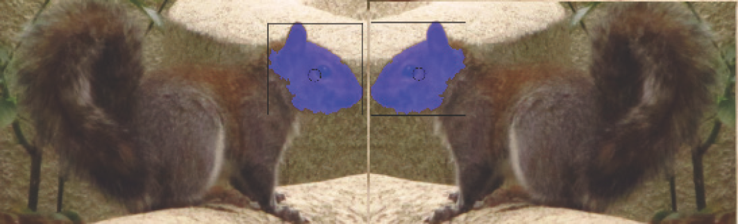
Table 11.9: Uniform metrics comparison scores for left head:right head genomes in Figure 11.14


Test Genome Correspondence Scoring Results
All compare metrics are weighted at 1.0 unless otherwise noted; these are raw first order metric scores without qualification and weight tuning applied. The metric correspondence scores all come out at reasonable levels, and some scores may be suitable as is with no additional tuning or learning beyond the built-in autolearning hull learning applied to all first order metric comparisons by the MCC functions. As expected, the left and right mirrored squirrel heads show the best correspondence and the stucco and squirrel head show the worst correspondence.
Note that not all the uniform compare metrics are useful in each case. Some are more reliable than others for specific test genomes, and as expected the optimal metrics must be selected and tuned using reinforcement learning for best results. The uniform base metrics used for scoring are summarized in Tables 11.10 and 11.11 below, including agent override criteria details.
Table 11.10: Uniform set of metrics for the test genome correspondence scoring
| Metric Category | Metric Spaces Computed Per Category | Agent Overrides |
| Color metrics | Proportional_SAD5 Sl_contrast_JensenShannon8 Popularity5_CLOSEST | MR_SMITH BOOSTED MR_SMITH NORMAL MR_SMITH NORMAL |
| Volume shape metrics | Centroid_8 Density_8 |
AGENT_RGBVOL_RAW AGENT_RGBVOL_MIN |
| Volume texture metrics | RGB VOL AVE of (0,45,80,135 GENOMES) R,G,B,L HSL_S AVE of (0,45,90,135 GENOMES) |
AGENT_RGBVOL_RAW AGENT_RGBVOL_AVE |
| SDMX metrics | SDMX AVE locus_mean_density SDMX AVE linearity_strength | MR_SMITH NORMAL MR_SMITH NORMAL |
| Haralick metrics | HARALICK CONTRAST (scaled uniformly using a weight of 10.0) | MR_SMITH NORMAL |
Table 11.11: Total base metrics computed for each test genome
| Metric Category | Total Metrics | Metric Spaces Computed Per Category |
| Color metrics | 1,800 | 15 metrics, 5 color space components [R,G,B,L,HLS_S], 4 color levels, 5 images [RAW,SHARP,RETINEX,HISTEQ,BLUR], 6 agents: total metrics 1800 = 15x5x4x6 |
| Volume shape metrics | 2,250 | 9 metrics, 5 color space components [R,G,B,L,HLS_S], 5 images [RAW,SHARP,RETINEX,HISTEQ,BLUR], 10 agents, total metrics 9x5x5x10 |
| Volume texture metrics | 1,200 | 4 metrics, 5 color space components [R,G,B,L,HLS_S], 5 images [RAW,SHARP,RETINEX,HISTEQ,BLUR], 12 agents, total metrics: 4x5x5x12=1200 |
| SDMX metrics | 165 | 11 metrics, 5 angles, 3 images [RAW,SHARP,RETINEX], I color LUMA: total metrics: 11x5x3x1=165 |
| Haralick metrics | 12 | 4 metrics, 3 images [RAW,SHARP,RETINEX], 1 color LUMA, total metrics: 4x3x1=12 |
| ALL TOTAL | 5,427 | Total of CSV metric comparisons made for each genome compare |
A total 5,427 base metrics are computed for each genome comparison by the CSV agents, as shown in Table 11.11 and then compared using various distance functions as discussed in Chapters 6–10. The final correspondence scores are summarized in Table 11.12, showing that the uniform set of metrics used in this case does in fact produce useful correspondence. The CSV agents used to collect the test results include built-in combination classification hierarchies as well as metrics qualifier pairs and weight adjustments (see Chapter 4 and the open source code for CSV agent for details).
In an application, using a uniform set of metrics for all genome comparisons is usually not a good idea, since each genome still corresponds best to specific learned metrics and tuning. In other words, each reference genome is a separate ground truth, and the best metrics to describe each reference genome must be learned, as well as adding qualifier metrics tuning using trusted and dependent metrics as discussed in Chapter 4. Therefore, each genome is optimized for correspondence by learning its own classifier.
Scoring Results Discussion
Scoring results for all tests are about as expected. Table 11.12 summarizes the final scores. Note that even using only first order metric scores for the tests, the results are good, and further training and reinforcement learning would improve the scoring. Note that the left/right head genome mirrored pair are expected to have the best cumulative scores, as observed in Table 11.12, while the enhanced back and rotated back are very similar and do match, revealing robustness to rotation and color similarity. The other genome scores show nonmatches as expected. For scoring, the MEDIAN may be preferred instead of the AVE if the scores are not in a uniform distribution or range, as is the case for the front squirrel/stucco compare scores (see Table 11.12).
Table 11.12: Test correspondence scores (< 1.0 = MATCH, 0 = PERFECT MATCH)

*NOTE: Adjusted score is the average of the AVE+MEDIAN. Other adjusted score methods are performed by each CSV agent.
To summarize, the test metric correspondence scores in Table 11.12 are first order metrics produced by the CSV agents and MCC functions using default agent learning criteria and default overrides. No second order tuned weights are applied to the scores. Also note that the test scores in the preceding individual genome tests show that not all the metrics are useful in a raw first order state and need qualification pair and tuning to incorporate into an optimal learned classifier.
Scoring Strategies and Scoring Criteria
The master learning controller (MLC) would select a similar set of metrics similar to those in Table 11.4 and then create qualifier metrics and dependent metric tuning weights for a series of tests. As discussed in the “VGM Classifier Learning” section of Chapter 4, we can learn the best scoring feature metrics to reserve as trusted metrics and then qualify and weight dependent metrics based on the strength of the trusted metrics scores. Using qualifier metrics to tune dependent metrics is similar to boosting strategy used in HAAR feature hierarchies (see [168]).
However, scoring criteria are developed using many strategies, none being a perfect strategy. If the trainer decides that the sky is red, and the metrics indicate that the sky is blue, the metrics will be adjusted to match ground truth (“No, the sky should be red, it just looks blue; tune the metrics to make the sky look red, minimize this metric contribution in the final classifier, and adjust the training set and test set to make it appear that the sky is actually red.”). This is the dilemma of choosing ground truth, training sets, test sets, metrics, distance functions, weight tunings, and classifier algorithms.
Unit Test for First Order Metric Evaluations
This section contains the results for three unit tests and is especially useful to understand genome ground truth selection and scoring issues. The unit tests computing correspondence between visually selected genome pairs, intended to explore cases where the human trainer has uncertainty (close match or maybe a spoof), as well as where the human trainer expects a match or nonmatch. The tests provide only first order comparisons against a uniform set of metrics that are not learned or tuned. The unit tests include a few hundred genome compare examples total—valuable for building intuition about MCC functions.
Unit Test Groups
The test groups are organized by creating named test strands containing a pair of genomes to compare as follows:
–GROUP 1: MATCH_TEST: The two genomes look like a match, based on a quick visual check. The metric compare scores in this test set do not all agree with the visual expectation, and this is intended to illustrate how human and machine comparisons differ.
–GROUP 2: NOMATCH_TEST: The two genomes do not match, based on a quick visual check. This is expected to be the easiest test group to pass with no false positives.
–GROUP 3: CLOSE_TEST: The genomes are chosen to look similar and are deliberately selected to be hard to differentiate and cause spoofing. This test group is the largest, allowing the metrics to be analyzed to understand details.
For the unit tests, the test pairs reflect human judgment without the benefit of any training and learning. Therefore, the test pairs are sometimes incorrectly scored, intended to demonstrate the need for refinement learning and metrics tuning. Scoring problems may be due to (1) arbitrary and unlearned metrics being applied or (2) simply human error in selecting test pairs.
Unit Test Scoring Methodology
The scoring method takes the average values from a small, uniform set of metrics stored in CSVs for shape, color, and texture, as collected by the ./vgv RUN_COMPARE_TEST command output; a sample is shown below. The metrics in the CSV are not tuned or reinforced as optimal metrics, and as a result the average value scoring method used is not good and will be skewed away from a more optimal tuned metric score. The unit tests deliberately use nonoptimal metrics to cause the reader to examine correspondence problems to force analysis of each metric manually, since this exercise is intended for building intuition about metric selection, tuning, and learning. The complete unit test image set and batch unit test commands is available in the developer resources in open source code library, including an Excel spreadsheet with all metric compare scores as shown in the ./vgv RUN_COMPARE_TEST output below.
Each unit test is run using the vgv tool (the syntax is shown below), where the file name parameters at the end of each vgv command line (TEST_MATCH.txt, TEST_NOMATCH.txt, TEST_CLOSE.txt) contains the list of strand files containing the chosen genome reference and target pairs encode in individual strand files. The strand reference and target genome pairs can be seen as line-connected genomes in the test images shown in the unit tests in Figures 11.15, 11.16, and 11.17.

The final score for each genome pair compare is computed by the CSV agent agent_mr_smith() using a generic combination of about fifty CTS metrics, heavily weighted to use CAM clusters from volume projection metrics. Without using a learned learned classifier, metric qualification, or tuning, the scoring results are not expected to be optimal and only show how good (or bad) the autolearning hull thresholds actually work for each metric compare.
For example, compare metrics produced by agent mr_smith NORMAL are shown below for a genome comparison between the F18 side (gray) and the blue sky by the giant Sequoia trees (see Figure 11.17). The final average scores are shown at the end of the test output, as a summary AVE score of color, shape, and texture scores. Also, the independent AVE scores for color, shape, and texture are listed as well, showing that the color score of 6.173650 (way above the 1.0 match threshold) is an obvious indication of the two genomes not matching.


As shown in the test output above, the volume projection metrics (CAM neural clusters) show quite a bit of variability according to the orientation of the genome comparison (A, B, C, or D). Using the average orientation score does not seem to be very helpful. Rather, simply selecting the best scoring orientation from each CAM comparison and culling the rest would certainly make sense as a metric selection criteria, followed by a reinforcement learning phase. The color and texture metrics show similar scoring results, illustrating how metrics selection must be learned for optimal correspondence.
MATCH Unit Test Group Results
The MATCH test genome pairs are connected by lines, as shown in Figure 11.15. Each MATCH pair is visually selected to be a reasonable genome match. The final AVE scores for each genome compare are collected as shown in Table 11.13 and reflect no metric tuning or reinforcement learning. The results show mainly good match scoring < 1.0, which is to be expected in this quick visual pairing. However, the scoring results generally validate the basic assumptions of the VGM volume learning method.

Table 11.13: MATCH scores from genome pairs in Figure 11.15

NOMATCH Unit Test Group Results
The NOMATCH test genome pairs shown in Figure 11.16 are selected to be visually obvious nonmatches for false positive testing. The final AVE scores are collected 11.14, reflecting no metric tuning or reinforcement learning. The results show zero matches scoring < 1.0, which is to be expected, and generally validates the basic assumptions of the VGM volume learning method.

Table 11.14: NOMATCH scores from genome pairs in Figure 11.16

CLOSE Unit Test Group Results
The CLOSE test genome pairs shown in Figure 11.17 are selected to be visually close to matches, but are intended to fool the scoring and metric anomalies for further study. The final AVE scores are collected as shown in Table 11.15, reflecting no metric tuning or reinforcement learning. The results show only three matches scoring < 1.0, with a few other scores close to 1.0, validating the intent of the test.

Table 11.15: CLOSE scores from genome pairs in Figure 11.17

Agent Coding
Basic boilerplate agent code is provided below, illustrating one method to write a basic agent to: register a custom agent, receive sequencer pipeline callbacks, receive correspondence callbacks, and start and stop the pipeline. This section is intended to be brief, since the VGM open source code library contains all the information and examples needed to write agent code. See Chapter 12 for details on open source code.


Summary
This chapter lays the foundation for VGM application development, using interactive training to learn strands of visual genome features of a squirrel and other test set genomes. The training process illustrates how each reference genome is a separate ground truth item—with its own learned classifier using the autolearning hull and the best learned metrics, which shloud be tuned via reinforcement learning using qualifier metrics to learn a structured classifier. To illustrate the process and build intuition, a small set of test genomes is selected using the interactive vgv tool, and then CSV agents are used to collect and compare metrics between test genomes. Reinforcement learning details are illustrated by walking through the process of evaluating genome comparison scores, with discussion along the way regarding scoring criteria and scoring strategies. A set of three unit tests are executed to evaluate cases where the genomes (1) visually match, (2) might match, and (3) do not match. Finally, brief sample agent code is provided as an example of how to run through the VGM pipeline.