Single-Image vs. Multiple-Image Strands

Strands can be composed from genomes collected from a single-image segmentation or from genomes spanning multiple-image segmentations. Combining genomes from several segmentations of an image is also possible. Single-image strands are the default method for convenience because all the segmentation boundaries line up within the image with no overlap. Single-image strands are simple to visualize and supported by the online tools described in Chapter 5. However, a strand may be constructed from genomes spanning multiple segmentations of the same image under various pre-processing and segmentation parameters for better results. In Chapter 11, several practical guidelines for creating single-image and multiple-image strands are provided.

For strands constructed from multiple images and multiple segmentations, the genome region boundaries may overlap, which is okay (see Figure 8.1). In this case, the agent may simply collect chosen genomes together into a group and manage correspondence at the genome level, one compare at a time, instead of using VGM platform convenience functions which are intended for single-image strands.

Strand Local Vector Coordinate System

Strands exist within a local vector coordinate system to define the relative distance and angles between each genome in the strand. As discussed in Chapter 3, the strand includes a start point (primary), end point (terminal), and genome location point (G) for each strand member (see Figure 8.2).

The length between the primary and terminal genomes is the unit length used to normalize all vector lengths in the local coordinate system, and the angle between the primary and terminal is unit angle 0, also used for normalizing angles. The intermediate genome order in the strand is arbitrary. The blue line shows a bidirectional vector between the primary and terminal genome centroids. The green lines are the vectors between the primary and intermediate genomes, and the red lines show the vectors between the terminal and intermediate genomes. The separate primary and terminal strand local coordinate systems provide a fail-safe mechanism, in case either the primary or terminal strand genome is not found, as shown in Figures 8.3 and 8.4 and discussed next.

By using both a primary and terminal genome as vector origins, a fail-safe mechanism is created, whereby either the primary or terminal vector can be missing in a target strand. Yet, the coordinate system can be reconstructed from either the primary or terminal by recomputing the unit length and unit angle between any two known reference points in the strand. For example, if the primary is found, but not the terminal, the strand local coordinate system can be rebuilt using the primary P and another genome Gn in the strand PGn.

A strand local vector coordinate system can be implemented by agents several ways besides the default method, as follows:

–Strand local relative coordinate system, where each genome is normalized to the PT vector length and PT angle. (*This is the default method.)

Strand Vector Metrics

Strands are compared based on the vector relationships and correspondence scores of each individual genome between a pair of strands. The default strand vector comparison functions fall into two types:

The concept of comparing a reference strand to a target strand is illustrated in Figure 8.5, which introduces the idea of locating and culling candidate genomes from the target strand to prepare for strand correspondence. The strand location and strand correspondence process is described in detail in this section.

As shown in Figure 8.5 we see a reference strand SR (left) and a target strand ST candidate (right), which is not identical to the reference strand and is a candidate only. The target strand ST candidate is created by searching a target image for the best match to each genome Gn in the reference strand SR, searching for candidate genomes Cn to compose into the target strand ST. MCC functions are used to locate candidates. The vector angle and magnitude of each candidate target genome in relation to the primary and terminal is recorded as well. Correspondence criteria for this example are discussed next.

SR contains 10 genomes [ P, G1…G8, T]. Note that there is only one P candidate in ST, and this is important since establishing the primary genome is critical to establishing the strand local coordinate system. The target strand ST of candidate genomes Cn is contained in a larger bounding box region than the reference strand SR, which may indicate a scale change if the candidates prove to correspond to the reference. Note that the candidate strand ST shows 13 candidate genomes Cn, with the most unlikely candidates culled and marked with a red cross-out symbol, based on the mismatch of vector distance and magnitude within the local coordinate system, as follows:

Two C1 candidates for G1 (one culled based on angle)

One C2 candidate for G2

Missing candidate C3 for G3

One C4 candidate for G4

Two C5 candidates for G5 (one culled based on angle)

One C6 candidate for G6

One C7 candidate for G7

Two C8 candidates for G8 (one culled based on angle)

One P primary candidate

As explained in Chapter 3, the strand model provides parameters to mark each genome in the strand as optional and also to weight each genome for scoring contribution. The default MCC strand correspondence functions provide a threshold parameter for culling candidate genomes, if the vector magnitude or angle are out of bounds beyond the threshold. The final score is computed based on the combined scores of all attributes of the candidate genomes in the target strand. The scoring is computed by MCC functions and includes MIN, AVE, and MAX scoring.

The default MCC function signatures for strand correspondence are shown in the following code snippet. Note that the match__find_strand_candidate() function is called first to build a candidate strand, and then the match__strand_correspondence() function is called to compute strand correspondence genome by genome, with the option to compute various shape descriptors as shown in Figure 8.6. The criteria parameter is used to apply heuristics to the match functions and is defined in Chapter 5 in the “CSV Agents” section. Note that strand management functions are discussed in Chapter 5 also, which allow for registration and access to strand structures.

Strand Set Metrics

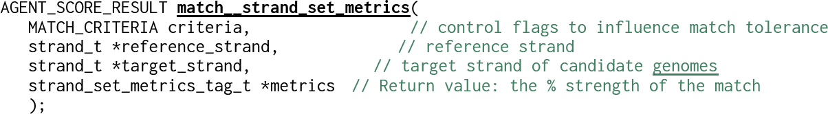
Strands, which are sets of genomes, can be compared using set metrics with the default match__strand_set_correspondence() convenience function, which operates on a reference and target strand structure, providing the metrics shown in the following code snippet. Also, strand metrics can be accessed directly from the global metrics compare structure discussed in Chapter 5. Note that this function is intended for single-image strands, as discussed earlier in this chapter, rather than multi-image strands.

Strand Shape Metrics: Ellipse and Fourier Descriptors

The genome centroids in a strand provide a basis for a 2D shape metrics. As shown in Figure 8.6, a strand can be analyzed in terms of shape. The Fourier descriptor [121][1] contains a Fourier series showing the circularity of the genome centroid distribution. Also, an enclosing ellipse descriptor provides a very rough outline of the containment of all genomes in the strand, including metrics for a normalized major and minor axis length and angle, as well as a centroid position for the ellipse and a bounding box. A radial histogram SAD compare is also provided using a 256-bin histogram of the vector lengths from the ellipse centroid to each genome centroid (see [1]).

The strand shape metrics are obtained using the following function. Note that this function is intended for single-image strands, as discussed earlier in this chapter, rather than multi-image strands.

Statistical Metrics

The statistical metrics are created during the volume projection process, as discussed in Chapter 6, and include centroid (usually the most useful), full/empty counts, maximum neuron address, and largest neuron count, discussed next.

Each statistical volume projection shape metric is available in the global compare metric structure discussed in Chapter 5 and also via MCC convenience functions shown in Table 8.1 at the end of the chapter.

Centroid Correspondence, Volume Space Alignment

The centroid is the largest volume bin value in each x,y,z axis, marking the center point of address distribution (i.e. the center of the neural cluster) which is the most common 24-bit address in the volume. (NOTE: This is not a mass centroid that uses a weighted center of all address contributions.) The x,y,z volume centroid, as shown in Figure 8.7, has the interesting property of providing a simple, very good first-pass correspondence metric, discussed in the next section.

Volume spaces can be aligned prior to MCC correspondence, and the centroid is a good alignment point. Since genome volume centroid alignment is usually a valuable indicator of genome similarity, the centroid can also be used to add lighting invariance to volume comparisons by aligning volumes prior to comparison, similar to the color alignment methods such as sliding histogram compare and centroid alignment MCC functions discussed in Chapter 6. A future VGM version will also provide additional volume alignment methods following those in Chapter 6 for 2D color regions. For example, the reference genome can be centroid-aligned to the target genome centroid prior to using the MCC distance functions shown at the end of this chapter. The default MCC behavior is no centroid alignment. Agents are free to align features using any method prior to correspondence, such as centroid or other shape factors. A function is provided to centroid-align the reference and target genome volumes prior to correspondence and also a command line option to the vgc command is provided as well (see Chapter 5).

The volume centroid delta metrics for Figure 8.7 are listed here for the A_0 genome in 8-bit resolution and 5-bit resolution. The centroid delta is the absolute difference between the reference and target genome centroids. Note that 8-bit resolution is most reliable for the centroid comparison metrics.

The x,y,z centroids of two volume projections, reference = r and target = t, are compared using a heuristic matching function via simple differencing to produce the centroid delta metric as follows:

$\begin{array}{l}{c}_{delta}=\frac{\left(\left|c_x^r-c_x^t\right|+\left|c_y^r-c_y^t\right|+\left|c_z^r-c_z^t\right|\right)}{3},\\ if\left(c_{delta}<10\right)thenMATCH\\ where{c}_{x,y,z}^{r}arereferencecentroids,and{c}_{x,y,z}^{t}aretargetcentroids\end{array}$

For example, the data table above provides a set of volume centroid deltas comparing the two window genomes in Figure 8.7. Line 1 provides the 8-bit centroid delta in the GENOME_A_0_DEGREES RETINEX LUMA space. The delta is 5,4,5; therefore the average centroid value is ca = (5+4+5)/3 = 4.7. So according to eq. 8.1, 4.7 is < 10 and is considered a match.

Full/Empty

The full/empty metrics show the number of volume projection cells that are full (occupied, count > 0) in each neural cluster. For reference, the different numbers of volume cells for each bit quantized space is shown here:

MAX Neuron Address

The max metric provides the x,y,z volume address of the neuron with the largest address accessed in the neural cluster as a binary formatted centroid address for each quantization space.

Ratio Metrics

The ratio metrics are based on combinations, or ratios, of the statistical volume projection metrics. Several ratios could be devised, but the default ratio metrics are shown in this section. They are also present in the base global metrics and metric compare structures discussed in Chapter 5. Ratio metrics are most useful combined as dependent metrics discussed in Chapter 4, with other more reliable metrics in a multivariate classification. Each metric is computed across (8, 5, 4, 3, 2 bit) quantizations, (raw, sharp, retinex, histeq, and blur) image spaces, and combined with each color channel (r, g, b, luma, RGB_volume), for a total of 5x5x5 = 125 metrics for each ratio.

Displacement

For images with very low or smooth texture, there will be a small range of pixel values and a corresponding small number of volume cells accessed. Displacement measures the percentage of volume cells that are used.

Density

This metric provides a gross indication of the average neuron size in the neural cluster. Larger relative sizes indicate a smaller distribution of pixel values which may indicate a better segmentation.

Spread

The spread provides a gross indication of the pixel value distribution in the 2D genome images.

Genome Structure Local Feature Tensor Space

The genome internal shape structures do not contain a strand local coordinate system, but instead rely on strands of glyph feature descriptors within a single genome, within the genome’s local feature tensor space, with interest point angle, interest point magnitude, and the feature descriptor value. The feature descriptors supported in the VGM are COLOR_HUE_SATURATION_SIFT, LUMA_GSURF, and LUMA_ORB. So for each glyph space, a genome local feature tensor space is represented with invariance to rotation, scale, and feature strength magnitude. Note that ORB is probably the most invariant to rotation and scale and may be the most reliable local descriptor overall (see [1].)

The local feature tensor space for each glyph feature is recorded in the strand. A genome may contain several features and corresponding tensors. As shown in Figure 8.8, each genome structure strand contains a tensor for each feature descriptor with the following information:

Feature descriptor structure tensor: (<x,y><θ><m><s><t><v>)

<x,y> location

<θ> orientation

<m> magnitude

<s> sign (blue is negative, red is positive)

<t> type of feature descriptor

<v> value of feature descriptor

As shown in Figure 8.8 (left), the orientation and magnitude of the GSURF Hessian-based interest points are shown using a yellow line, and the sign of the Hessian determinant at the interest point is shown using a red origin for positive values (local extrema) or blue origin for negative values (not an extrema; perhaps a candidate for culling). This information is preserved in the tensor for each feature.

The function signatures for creating genome local feature strand structures and the correspondence metrics function are shown below. Note that these strand functions are intended only for strands created from a single image, as discussed earlier in this chapter, rather than multi-image strands.

Genome Structure Correspondence Metrics

The correspondence metrics for genome structure strands are combined together into a common MCC function, shown in the following code. Note that the genome structure strands must be built using the build_structure_strand() function discussed in the previous section so that the structure is compatible for use with the MCC strand correspondence function match__structure_strand_features() shown here.

The metrics provided include (1) the average score of feature comparisons below a sanity threshold, (2) the number of features compared below the sanity threshold, and (3) the percentage of compared features that matched. Note that the process for determining genome structure strand correspondence metrics is shown here: