Chapter 2
Eye/LGN Model
The eye is not satisfied with seeing.
—Solomon
Overview
In this chapter we model a synthetic eye and a synthetic lateral geniculate nucleus (LGN), following standard eye anatomy [16][1] and basic neuroscience covered in [1] Chapters 9 and 10. First, we develop the eye model emphasizing key eye anatomy features, along with types of image processing operations that are biologically plausible. Next, we discuss the LGN and its primary functions, such as assembling optical information from the eyes into images and plausible LGN image processing enhancements performed in response to feedback from the visual cortex. We posit that the LGN performs image assembly and local region segmentations, which we implement in the VGM.
Eye Anatomy Model
As shown in Figure 2.1, a basic eye model provides variable focus, blur, sharpness, lightness, and color corrections. The eye model does not include geometric or scale transforms. Fortunately, digital cameras are engineered very well and solve most of the eye modeling problems for us. Standard image processing operations can be used for other parts of the eye model.
The major parts used in the synthetic eye model are:
–An aperture (pupil) for light control.
–A lens for focus.
–A retina focal plane to gather RGBI colors into pixel raster images via rods and cones.
–Standard image processing and a few additional novel algorithms. These are provided in the API to perform plausible enhancements to color and resolution used for higher-level agent hypothesis testing, as discussed in Chapter 6.

Here we describe the anatomical features in Figure 2.1.
Iris—The iris muscle is the colored part of the eye and ranges in color from blue to brown to green and rarer colors. The iris controls the aperture (pupil) or amount of light entering the eye. By squinting the eye to different degrees, a set of images can be observed at differing light levels, similar to the high dynamic range (HDR) methods used to create image sets in digital cameras.
Lens—The lens muscle controls the focal plane of the eye, along with the iris muscle, allowing for a set of images to be observed at different focal planes, similar to the all-in-focus methods used by digital cameras. The lens can be used to change the depth of field and focal plane.
Retina—The retina is the optical receptor plane of the eye, collecting light passing through the iris and lens. The retina contains an arrangement of optical cells (magno, parvo, konio) containing rods and cones for gross luminance and red, green, blue (RGB) color detection. The retina encodes the color information into ganglion cells which feed the left/right optical nerves for transport into the left/right LGN processing centers.
Fovea—The fovea is the region in the center of the retinal focal plane, containing color-sensitive red and green cone cells. The blue cones are in the periphery region of the retina outside the center foveal region.
Rods—Rods are more sensitive to low light and fast moving transients than cones and track motion. Rods are sensitive to lightness (L) which overlaps the entire RGB spectrum. Rods are the most common visual receptors. Rods are almost insensitive to red (slowest RGB wavelength light), but highly sensitive to blue (fastest RGB wavelength of light), and note that the blue cones are also located in the periphery of the retina with the rods. The rods are located almost entirely in the periphery of the retina, along with the blue cones, and perform periphery vision. About 120 million rods are located outside the primary foveal center of the retina. Rods are about 10x–15x smaller than cones.
Cones—Sensitive to color (RGB). Cones are most sensitive when the eye is focused—when the eye is saccading (dithering) about a focal point. There are approximately 7 million cones: about 64% of which are red cones, 32% green cones, and 2% blue cones. The red and green cones are located almost entirely within the foveal central region. However, the blue cones are located in the peripheral region of the retina along with the rods. The blue cones are highly light sensitive compared to the red and green cones. However, the human visual system somehow performs RGB processing in such a way as to allow for true RGB color perception. Cones are 10x larger than rods. See Figure 2.2.

Visual Acuity, Attentional Region (AR)
We are interested in modeling the retina’s fovea attentional region (AR) of focus size in pixels, which of course varies based on the image subject topology, distance, and environmental conditions such as lighting. Since an entire visual acuity model is quite complex, we only seek a simple model here to guide the image segmentation region sizes. For information on visual acuity in the human visual system we are informed by the “Visual Acuity Measurement Standard,” Consilium Ophthalmologicum Universale [22].
For practical purposes, the AR is used for model calibration to determine a useful minimum size for segmented regions containing metrics and feature descriptors. We use the AR to model the eye anatomy of the smallest size region of pixels currently under focus. As shown below for several parvo scale image examples, we work out the size of a typical AR for a few images to be typically ~30x30 pixels, depending on image size and quality, which helps guide parameterization of segmentation and image pre-processing, as well as culling out segmentations that are way too large or small.
The highest density of rods and cones is toward the retina’s very center at the fovea. Rod and cone density falls off toward the periphery of the field of view (FOV), as shown previously in Figure 2.2. Visual acuity is a measure of person’s ability to distinguish fine detail at a distance and varies widely among subjects, otherwise referred to as near sightedness and far sightedness. In general, the region of acuity is limited in size to allow for focus on textural details and color, and to define the size of segmented genome regions.
The foveal area that is under attention in the center of the FOV subtends an angle of perhaps 0.02–0.03 degrees in the oval retinal field of view, which is a small percentage of the entire FOV. The magno cells take in the rest of the image field of view with less detail. For our simplified model, we define the foveal region in a rectangular image space of perhaps 0.01% of the total FOV in a rectangular image. The rest of the image is not in best focus, under view of mainly rod cells, and not viewed under the highest detail cone cells. We call the center of the FOV under focus the attentional region (AR).
To simulate the AR in our simplified visual model, we take the total parvo image size and then compute an AR value to be about 0.01% of the total image, and use the AR for guidance when segmenting the image to identify the minimum segment size segmented regions to cull. For parvo scale images:
Note that if segmentations are carried out in magno space, the minimum area sizes should be considered as 5x smaller than the corresponding parvo scale ARs shown above, so magno segmentations are scaled up 5x to match parvo scale prior to using the segmented regions on the parvo image to compute metrics. In other words, the magno segmentations are the borders; the parvo image pixels fill in the borders for the segmented region. However, segmentations can be computed directly on the parvo scale image, and then a magno scan can be used together with a parvo scan in the model. Since no single segmentation is best for all images, a magno and parvo segmentation used together is a reasonable baseline. However, currently we prefer only parvo segmentations for metrics computations since color information and full resolution detail is included.
In practice, we have found interesting features in regions smaller than 0.01% of the total image pixels and have seen useful features in AR regions as small as 0.005%–0.02%. However, this is purely an empirical exercise. In future work, each segmented region will be resegmented again to reveal embedded higher-resolution segments. Also note that the shape of the regions varies depending on the segmentation algorithm and parameters used, so area alone is not always helpful—for example, the bounding box size and other shape factors can be used to guess at shape.
We therefore have empirically arrived at a minimum useful parvo segment size parameter for the AR which varies between 0.01% and 0.015% of the total pixels in the image, depending of course on the image content. Note that our default region size was determined empirically using a range of images, pre-processing methods, and segmentation methods. However, our empirical AR value matches fairly well with our mathematical model of the retina and fovea regions. At about 30cm from the eye, the best human visual acuity of 6/6 can resolve about 300 DPI (pixels per inch), which is about 0.05% of the available pixels in a 5MP image at 30cm, and at 1 meter, the value becomes an area with a size of about 0.005% of the total pixels, which approximates our default foveal region size chosen and tested with empirical methods.
The human eye also dithers and saccades rapidly between adjacent regions to increase the level of detail and test hypotheses such as color, texture, and shape. So, several segments are kept under attention simultaneously in order to arrive at a synergistic or summary classification of a collection of segments.
LGN Model
For the synthetic model, we model the LGN (lateral geniculate nucleus) to perform the following functions:
–Camera: The LGN acts as a digital camera to assemble rods and cones into raster images.
–Image assembly and representation: The LGN assembles images from its camera to feed into the magno and parvo pathways which feed the visual cortex, including stereo image assembly and color image assembly.
–Enhancements: The LGN performs high-level image processing and enhancements as directed during hypothesis testing, such as contrast corrections and other items discussed below.
–Segmentations: We model segmentation in the LGN for convenience and posit that the LGN performs image processing related to segmentation of the image into regions based on a desired similarity criteria, such as color or texture, in cooperation with the visual cortex.
Next we will discuss each LGN function in more detail.
LGN Image Assembly
The LGN basically assembles optical information together from the eyes into RGBI images: RGB comes from the cones, and I from the rods. The LGN evidently performs some interesting image processing such as superresolution via saccadic dithering, high dynamic range imaging (HDR), and all-in-focus images.
Our purposes do not demand a very detailed synthetic model implementation for the LGN camera section, since by the time we have pixels from a digital camera, we are downstream in the visual pathway beyond the LGN. In other words, for our purposes a digital camera models most the eye and LGN capabilities very well.
The LGN aggregates the parallel optical nerve pathways from the eye’s magno neuron cells (monochrome lightness rods I), parvo neuron cells (red and green cones R, G), and konio neuron cells (blue cones B). The aggregation is similar to compression or averaging.
According to Brody [17], there is likely feedback provided to the LGN from V1, in order to control low-level edge enhancements, which we discuss more along with the V1–V4 model in Chapter 3. Little is known about feedback into the LGN. Feedback into the LGN seems useful for enhancements during hypothesis testing round-trips through the visual pathway. We postulate that the LGN is involved in low-level segmentations and receives feedback from the visual cortex during segmentation. The VGM API provides a wide range of biologically plausible enhancements emulating feedback into the LGN for color and lighting enhancements, plausible edge enhancements, focus, and contrast enhancements allowed by eye biology as discussed in Chapters 6, 7, 8, and 9.
As shown in Figure 2.3, gray-scale cones are aggregated together by magno cells, RG rods are aggregated together into parvo cells, and the blue cones are aggregated together in kino cells. The magno, parvo and kino cells send aggregated color information down the optical pathway into the LGN. Note that rods are about 10x–15x smaller than cones, as shown in Figure 2.3. The larger magno cells aggregate several rods, and smaller parvo cells aggregate fewer cones.

Magno neuron cells (L)—Magno cells, located in the LGN, aggregate a large group of light sensitive rods into strong transient signals. Magno cells are 5x–10x larger than the parvo cells. Perhaps magno cells are linked with blue cones as well as rods, since the blue cones are located interspersed with the rods. The magno cells therefore integrate about 5x–10x more retinal surface area than the parvo cells and can thus aggregate more light together than a single parvo cell. Magno cells are therefore more sensitive to fast moving objects, and perhaps contribute more to low-light vision.
Parvo neuron cells (R,G)—Parvo cells, located in the LGN, are aggregators of red and green cones in the central fovea region, creating a more sustained in-focus signal. Parvo cells are smaller than magno cells, and aggregate fewer receptors than magno cells. The visual pathway somehow downstream combines the red, green, and blue cones together to provide color perception and apparently amplifies and compensates for the lack of blue receptors and chromatic aberrations. Perhaps since red is the slowest wavelength compared to green, more red cones are needed (64%) for color sensitivity than green (32%) since they are refreshed less often at the lower wavelength.
Konio neuron cells (B)—Konio cells, located in the LGN, are aggregators of the blue cones distributed in the periphery vision of the retina, not in the central foveal region with the red and green cones. Konio cells are less understood than the magno and parvo cells. Blue cones are much more light sensitive than red and green cones, especially to faster-moving transients, but since the blue cones are outside the foveal focus region, they are not in focus like the red and green cells, seemingly contributing chromatic aberrations between R, G, and B. The visual system somehow corrects for all chromatic aberrations. Perhaps the fast wavelength of blue light allows for fewer blue cones (2%) to be needed, since the blue cones are refreshed more often at the faster wavelength. Also, the rods have a spike in sensitivity to blue, so evidently the LGN color processing centers have enough blue stimulus between the magno and the kino cells.
LGN Image Enhancements
Here we discuss the major image enhancements provided by the LGN in our model.
–Saccadic dithering superresolution: The eye continually saccades or dithers around a central location when focusing on fine detail, which is a technique also used by high-resolution imagers and radar systems to effectively increase the sensor resolution. The LGN apparently aggregates all the saccaded images together into a higher-resolution summary image to pass downstream to the visual cortex. Perhaps the LGN plays a role in controlling the saccades.
–High dynamic range (HDR) aggregation images: The LGN likely plays a central role in performing image processing to aggregate and compress rapid sequences of light-varying images together into a single HDR image, similar to methods used by digital cameras. The finished HDR images are delivered downstream to the visual cortex for analysis. Likely, there is a feedback into the LGN from the visual cortex for HDR processing.
–All-in-focus images: Perhaps the LGN also aggregates sequences of images using different focal planes together into a final all-in-focus image, similar to digital camera methods, in response to feedback controls from the visual cortex.
–Stereo depth processing: The synthetic model does not support depth processing at this time. However for completeness, we provide a brief overview here. The visual pathway includes separate left/right (L/R) processing pathways for depth processing which extract depth information from the cones. It is not clear if the stereo processing occurs in the LGN or the visual cortex. Perhaps triangulation between magno cells occurs in the LGN similar to stereo methods (see [1] Chapter 1). We anticipate an RGB-DV model in a future version of the synthetic model, which includes RGB, depth D, and a surface normal vector V).
Depth processing in the human visual system is accomplished in at least two ways: (1) using stereo depth processing within a L/R stereo processing pathway in the visual cortex and (2) using other 2D visual cues associated together at higher-level reasoning centers in the visual pathway. As discussed in [1], the human visual system relies on stereo processing to determine close range depth out to perhaps 10 meters, and then relies on other 2D visual cues like shadows and spatial relationships to determine long range depth, since stereo information from the human eye is not available at increasing distances due to the short baseline distance between the eyes. In addition, stereo depth processing is affected by a number of key problems including occlusion and holes in the depth map due to the position of objects in the field of view and also within the horopter region where several points in space may appear to be fused together at the same location, requiring complex approximations in the visual system. We assume that modern depth cameras can be used when we enhance the synthetic model, providing a depth map image and surface normal vector image to simulate the LGN L/R processing.
LGN Magno and Parvo Channel Model
As shown in Figure 2.4, there are two types of cells in the LGN which collect ganglion cell inputs (rods, cones) from the optic nerve: magno cells and parvo cells. Of the approximately 1 million ganglion cells leaving the retina, about 80%–90% are smaller parvo cells with smaller receptive fields, and about 10%–20% are larger magno cells with a larger receptive field. The magno cells track gross movement in 3D and identify “where” objects are in the visual field, identifying objects sensitive to contrast, luminance, and coarse details (i.e. the receptive field is large and integrates coarse scene changes). The parvo cells are slower to respond, perhaps since the receptive field is small, and parvo cells represent color and fine details corresponding to “what?” the object is. Magno cells are spread out across the retina and provide the gross low-resolution outlines, and parvo cells are concentrated in the center of the retina and respond most during the saccadic dithering process to increase effective resolution and fill in the details within the magno outlines.
The magno and parvo cell resolution differences suggest a two-level spatial pyramid arrangement built into the retina for magno-subsampled low resolution and parvo high resolution. In addition, the visual pathway contains two separate parallel processing pathways—a fast magno shape tracking monochrome pathway and a slow parvo color and texture pathway. Following the magno and parvo concepts, the synthetic model provides (1) low-resolution luminance genomes for coarse shapes and segmentations (magno features) and (2) higher-resolution color and texture genomes (parvo features).

Following the dual parvo and magno pathways in the human visual system, we model parvo features as microlevel RGB color and texture tiles at higher resolution and magno features as low-level luminance channels at lower resolution, such as primitive shapes with connectivity and spatial relationships. The magno features correspond mostly to the rods in the retina which are sensitive to luminance and fast moving shapes, and the parvo features correspond mostly to the cones in the retina which are color sensitive to RGB and capture low-level details with spatial acuity. The central foveal region of the retina is exclusively RG cones optimized to capture finer detail and contains the highest density of cells in the retina. Blue cones B are located outside the fovea mixed in with the rods (as shown in Figure 2.2). Magno cell density becomes sparser toward the edge of the field of view. The LGN assembles all the RGBI information into images.
Magno and Parvo Feature Metric Details
VGM provides an input processing model consisting of a set of separate input images as shown in Figure 2.5, which reflect the processing capabilities of actual vision biology at the eye and into the LGN.
–Raw luminance images
–Raw RGB color images
–Local contrast enhanced images to emulate saccadic dithering using the biologically inspired Retinex method (see Scientific American, May 1959 and December 1977)
–Global contrast normalization similar to histogram equalization to mitigate shadow and saturation effects and provided higher dynamic range
–Sharpened images emulating focus and dithering for superresolution
–Blurred images to emulate out-of-focus regions
–*NOTE: LBP (linear binary pattern, see [1]) images are supported on each RGBI channel, although perhaps not biologically plausible in the visual pathway
Following the magno and parvo cell biology, VGM computes two types of features and two types of images in a two-level feature hierarchy:
–Parvo feature metrics: Parvo features are modeled as RGB features with 100% full resolution detail, following the design of parvo cells; take input images at full resolution (100%); use RGB color; and represent color and texture features. Parvo cells are slower to respond to changes and integrate detail during saccades.
–Magno feature metrics: Magno features are modeled as lower resolution luminance features, following the magno cell biology and chosen to be scaled at 20% of full resolution (as a default approximation to magno cell biology). We posit that the larger magno cells integrate and subsample a larger retinal area; therefore we model magno cells at a lower resolution image suited for the rapid tracking of shapes, contours, and edges for masks and cues.

The parvo texture features are collected in four oriented genome shapes A, B, C, D (introduced in Chapter 6) within overlapped input windows, simulating the Hubel and Weiss [146,147] low-level primitive edges found in local receptive fields and also corresponding to Brodal’s oriented edge shapes [14]. The A, B, C, D oriented shapes are also discussed in detail in Chapter 9 as low-level textures.
Scene Scanning Model
To guide the synthetic model design and implementation, we assume that the human visual system scans a scene in a series of recursive stages, arranged in a variable manner going back and forth between stages according to the current task at hand and as directed by the agents in the higher learning centers. See Figure 2.6.

Scene Feature Hierarchy
The scene scanning processing stages result in a feature hierarchy across the bases CSTG:
- Magno object features
- Parvo object features
- Parvo micro object features
- Parvo nano object features
Here is an overview of the modeled feature scanning steps.
–Magno scene scan: This is a gross scene scan where the eye is roving across the scene primarily gathering luminance contrast, edge, and shape information; focus may be generally hazy and color information is not precise (global boundary scan). The eye is moving and covering a lot of ground.
–Magno object segmentation: The eye slows down to analyze on a smaller region, with increased focus to gather specific region boundary, edge, and texture information (local boundary scan). The eye is moving more slowly around a specific object. Decisions are made to categorize the object based on gross luma-contrast-based edge shape and contrast. The VGM records a shape mask (segmentation) representing this stage which can be further analyzed into shape moments and other metrics. Magno object VDNA metrics are computed and stored in the visual cortex memory.
–Parvo object segmentation: Using the culled and pruned segments from the magno segmentation, a color segmentation is performed on each preserved object segment with better focus and better parvo resolution. NOTE: Many parvo segmentations may be useful. During this stage, the eye is quickly moving and studying RGB features of each object segment. Decisions may be made at this level to categorize the object into a strand based mainly on color or texture metrics. Parvo object VDNA metrics are computed and stored in the visual cortex memory.
–Parvo interior scan: This scan produces a detailed color segmentation of microregions within the object, such as color textures, color space identification, color labeling, and small color boundaries. The eye is in fair focus over a small region covering perhaps a few percent of the center of the field of view, which contains a feature of interest such as a motif. The eye is moving slowly within the interest region but stopping briefly at key points to verify a feature. This stage is similar to the interest point and feature descriptor stage proposed in many computer vision models (see [1]). Parvo micro objects VDNA metrics are computed and stored in the visual cortex memory.
–Parvo nano stare: The retinex and histeq images are used in this stage, corresponding to the saccadic stage where the retina is closely studying, perhaps staring at a specifically focused point, dithering the focal point of the field of view in the AR, which area contains the smallest identifiable motif or detail of interest, such as a character, logo, or other small feature. Nano stares may also include recursive boundary scans to determine nano feature shape. This stage is similar to the interest point and feature descriptor stage proposed in many computer vision models (see [1]). Parvo nano objects VDNA metrics are computed and stored in the visual cortex memory.
–Strands: A proxy agent examines the genome region metrics from visual cortex memory and forms strands of related VDNA into one or more strands. Also, an existing strand can be decomposed or edited based on proxy agent hypothesis evaluations to add or remove segmentations and genome features. A strand is a view-based construct which can grow and increase in level of detail.
–Bundles: Bundles contain related strands, as composed by proxy agent classification results, and bundles can be edited to add or remove strands and features. As illustrated in Figure 2.6, the scanning occurs in semi-random order, so VDNA, strands, and bundles may change, since the proxy agent may direct the visual pipeline through various processing steps as needed, according to the current hypothesis under evaluation.
Based on the scene scanning model and assumptions just described, we proceed below to describe more specific model details for scene processing.
Eye/LGN Visual Genome Sequencing Phases
This section describes the phases, or steps, of our synthetic LGN model and posits that the visual pathway operates in four main phases which are recursive and continual (see also Figure 2.6):
- Gross scene scanning at magno resolution
- Saccadic dithering and fine detail scanning at parvo resolution
- Segmenting similar regions at both magno and parvo resolution
- Feature metric extraction from segments into visual cortex memory
We refer to visual genome sequencing analogous to the Human Genome Project as the process of disentangling the individual genome regions and VDNA, so segmentation is the primary step in sequencing to collect regions of pixel VDNA together.
To emulate the eye and LGN, we carefully prepare a set of images, as shown in Figure 2.7, representing the eye/LGN space of biologically plausible image enhancements. The eye and LGN can actually perform similar processing steps to those modeled in Figure 2.7, as discussed above in the section “LGN Image Enhancements.” Next, we go deeper to describe each sequencing phase and outline the algorithms used in the synthetic model.

Magno Image Preparation
We model magno response as a set of luminance images at 20% of full scale (see Figure 2.7). Apparently the visual system first identifies regions of interest via the magno features, such as shapes and patterns, during a scanning phase, where the eye is looking around the scene and not focused on a particular area. During the scanning phase, the eye and LGN model is not optimized for a particular object or feature, except perhaps for controlling gross lighting and focus via the iris and lens. The magno features are later brought into better focus and dynamic range is optimized when the eye focuses on a specific region for closer evaluation.
For the scanning phase and magno features, we assume a much simpler model than the parvo cells, since the magno cells are lower resolution and are attuned to fast moving objects, which implies that the LGN does not change the magno features as much from impression to impression. We take the magno features to be preliminary outlines only, which are filled in by details in the parvo cells. Our scanning model assumes the LGN perhaps changes parameters three times during scanning: (1) global scene scan at constant settings—magno cells filled in with very low-resolution info, (2) pause scan at specific location and focus to fill in more parvo RGB details, and (3) contrast enhance nano stare scan at paused position by LGN during saccades so the fine detail is captured from the parvo cells. Since magno cell regions contain several rods and are predominantly attuned to faster-moving luminance changes, our model subsamples luminance from the full resolution raw parvo images 5:1 (i.e. 20% scale), which seems to be a reasonable emulation of magno cell biology. Perhaps due to the larger size of the magno regions and the smaller size of the rods, (1) it is faster to accumulate a low-light response over all the cells in the magno region, and (2) the magno cell output is lower resolution due to the subsampling and accumulation of all the cells within the magno cell region.
Parvo Image Preparation
We model parvo response as a set of RGB images at full scale (see Figure 2.7). For closer evaluation, the visual system inspects interesting magno shapes and patterns to identify parvo features and then attempts to identify larger concepts. The eye saccades over a small active region (AR) within the larger segmentation regions. During saccades, the eye adjustments and LGN image enhancements may change several times according to the current hypothesis under attention by the high-level agent; for example, focus and depth of field may be changed at a particular point to test a hypothesis.
Segmentation Rationale
It also seems necessary to carefully mask out extraneous information from the training samples in a segmentation phase in order to isolate regions from which more precise feature metrics can be created. For example, masking out only the apple in a labeled image of apples allows for recording the optimal feature impressions for the apple, and we seek this feature isolation in the synthetic model. Human vision holds segmented regions at attention, allowing for further scanning and saccading as desired to study features. Segmented regions are therefore necessary to model the vision process. We choose to model segmentation in the LGN but assume feedback input comes from the visual cortex to guide segmentation. Note that DNN training often does not include segmented regions, perhaps since collecting hundreds of thousands of images to train a DNN is hard enough without adding the burden of segmenting or matting images to isolate the labeled training regions. However, some systems (i.e. Clarify) claim that masked, or segmented, training images work best when extraneous information is eliminated. Furthermore, some practitioners may argue that DNN training on segmented images is not wanted and even artificial, preferring objects embedded in their natural surroundings during training. The synthetic model does not require hundreds of thousands of images for training. Segmentation is therefore a simple concept to model, and desirable to effectively add biologically plausible training data samples into the model.
DNN semantic segmentation methods are improving, and this is an active area of research. However, DNN architecture limitations on image size preclude their use today in the current VGM, since 12MP images and larger are supported in the VGM. DNNs rescale all input images to a common size—perhaps 300x300- due to performance limitations. For more on DNN segmentation research, see [173][174] to dig deeper.
Segmentation seems to be ongoing and continuous, as the eye saccades and dithers around the scene responding to each new hypothesis from the PFC Executive. To emulate human visual biology and the LGN, there is no single possible segmentation method to rely on—multiple segmentations are necessary.
The VGM assumes that segmentation is perhaps the earliest step in the vision pipeline after image assembly. We scan the image a number of times, similar to the way the eye flickers around interesting regions to focus and gather information. Regions may be segmented based on a variety of criteria such as edge arrangement, shape, texture, color, LBP patterns, or known motifs similar to letters or logos which can be considered primal regions. We assume that the size of each region is initially small and close to the size of the AR region, which enables larger segmentations to be built up from smaller connected segmentations. There is no limit to the number of segmentations that can be used; however, more than one method to produce overlapping segmented regions is desirable, since segmentation is anomalous with no clear algorithm winner.
Effective segmentation is critical. Since we are not aware of a single segmentation algorithm which mimics the human visual system, we use several algorithms and parameter settings to create a pool of segmented regions to classify, including a morphological method to identify larger segments, and a superpixel method to create smaller, more uniformly sized segments. Both morphological and superpixel methods yield similar yet different results based on tuning parameters. In the future we intend to add an LBP segmentation method. We have tried segmentation on a variety of color space luma channels, such as RGB-I, Lab-L, HSV-V. We have tried a variety of image pre-processing steps prior to segmentation. We have also tried segmentation on color popularity images, derived from 5-bit RGB colors. We have not yet found the best input image format and processing steps to improve segmentations. And of course, we have also tried segmentation on the raw images with no image prepro-cessing. Based on experience, segmentation is most effective using a selected combination of superpixel methods [153–157], and for some images we like the morphological segmentation developed by Legland and Arganda-Carreras [20] as implemented in MorphoJlib.
Image segmentation is an active field of research, perhaps the most interesting part of computer vision. See Chapter 3 of [1] for a survey of methods and also the University of California, Berkeley Segmentation Dataset Benchmark competition results and related research. In addition, image matting and trimap segmentation methods can be useful, see the survey by Xu et al. [23]. A few notable papers on trimap segmentation and matting include [21][22]. A useful survey of the field of segmentation is found in [25]. Open source code for several color palette quantization methods and color popularity algorithms to segment and shrink the color space to common RGB elements is found at [26]. The Morpholib segmentation package is based on unique morphological segmentation methods and is available as a plugin for ImageJ Fiji [27], and a superpixel segmentation plugin for ImageJ Fiji can be found at [28]. Related methods to learn colors from images include [29][30]. See also [35] for a novel method of “selective search” using several region partitioning methods together for segmenting likely objects from images.
Segmentation Parameter Automation
While we provide a basic model for selecting segmentation parameters based on the image, future research is planned to develop a more extensive automated segmentation pipeline, which first analyzes the image to determine necessary image enhancements and segmentation parameters, based on a hypothesis parameter set (HPS) controlled by the agent. For example, each HPS could be composed to test a hypothesis under agent control, such as a color-saturation invariant test. The HPS follows the idea that the human visual system directs focus, dynamic range compensations, and other types of eye/LGN processing depending on the quality of each scene image and the hypothesis at hand. As explained earlier, the current VGM uses a few different types of processing such as histeq, sharpen, blur, retinex, and raw data at different stages in the model to mimic capabilities of the human visual system.
Currently, we use a modest and simple default HPS model, discussed next in the “Saccadic Segmentation Details” section.
Saccadic Segmentation Details
We optimize segmentation parameters to generate between 300–1500 segments per image as discussed later in this section, depending on image resolution. We cull out the segments which have a pixel area less than the AR size, and compute metrics over each region. Region size minimums of 200–400 pixels have proven to be useful, depending on the image resolution, as discussed earlier in the section “Visual Acuity, Attentional Region (AR).”
The details on the two basic segmentations we perform are discussed below:
–Magno LUMA segmentation: A segmentation over the pre-processed raw LUMA using magno 20% scale images which are then scaled up to 100% and used as the segmentation mask region over an RGB raw parvo scale image.
–Parvo RGB segmentation: A segmentation on the global histogram equalization parvo full-scale RGB image. Using multiple segmentations together mimics the saccadic dithering process.
Saccadic dithering likely involves integrating several segmentations over several saccades, so two segmentations is just a model default. Note that segmentation by itself seems to be the most important feature of the early visual pathway, since the segmentations allow region association and region classification. We have experimented with a model to emulate the magno pathway, focusing on the luminance information for the segmentation boundaries which seems not satisfactory. Somewhere likely in V1 or higher, the magno and parvo color channels are apparently combined into a single segmentation to evaluate color- and texture-based segmentations. In the VGM, we can combine magno and parvo segmentations using the agents. However, we postulate that the visual pathway contains a processing center (likely V1 or Vn) which is dedicated to merging the magno and parvo information into segments. At this time, we are still trying various methods to produce combined segmentation and have experimented with feeding HSV-H images to the segmenter, or Lab-L images, HIS-S images, color popularity-based images, etc., but without any satisfactory winner or fool proof rules or consistently winning results.
There are several statistical methods we have tried to analyze image texture to guide image pre-processing and segmentation parameter settings. For simplicity, the default model uses the Haralick Inverse Difference Moment (IDM) computed over a co-occurrence matrix (see Chapter 9):
As per the Figure 2.8 example, five different images and their corresponding Haralick IDMs are shown. We sort the IDM values into “texture threshold bands” (see Figure 2.8) to understand the fine texture details for parameter setting guidance.

Magno and parvo resolution segmentations are optimized separately, depending on the algorithm used: superpixel or morphological segmentation, and depending on the image resolution. Currently for 12MP images (4000x3000 pixels) we optimize the target number of segmentations as follows:
–For magno segmentation (~0.5MP images), we aim for 400 segments per image, and we cull out the segments which have a pixel area less than the AR size, or larger than a max size, yielding about 300–400 valid segments per image, each of which are considered a genome region.
–For parvo images (8MP–12MP images), we aim for about 2,000 segmentation and cull out small and large regions to yield about 1,000–1,500 segmentations.
From experience, we prefer superpixel segmentation methods, and more than one overlapping segmentation is valuable for best results, since no single segmentation is optimal. More work needs to be done for future versions of the model, and we describe possible enhancements as we go along. As shown in Figure 2.9, each segmented regions is stored in rectangular bounding boxes as a black/white mask region file and a separate RGB pixel region file. We use the rectangular bounding box size of the segmentation as the file size and set all pixels outside the segmented region to 0 (black) so valid pixels are either RGB values or 0xff for mask files. The segmentation masks from the raw image can be overlaid on all images to define the segmentation boundaries, so a full set of metrics are computed over each segmented region on each image: raw, sharp, retinex, global histeq, and blurred images. We refer to segmented regions as visual genomes, which contain over 16,000 different VDNA metrics. The raw RGB image metrics are the baseline for computing the autolearning hull, using retinex and sharp image metrics top define the hull boundary for matching features, as discussed in Chapter 4. Autolearning is similar to more laborious training methods, but only uses a small set of training images that are plausible within the eye/LGN model.

Processing Pipeline Flow
The basic processing flow for segmentation and metrics generation is shown in Figure 2.9 and described next, using a combination of ImageJ java script code and some descriptive pseudocode. Note that the synthetic model is mostly implemented in C++ code using massively parallel multithreading (not shown here).
Magno/Parvo Image Preparation Pipeline Algorithm
Magno image preparation is the same as parvo, except the raw image is first downsampled by 5x (by 0.2) to start. Pseudocode:

Segmentation Pre-Processing Pipeline
The Haralick IDM and other texture metrics are determined first, then the segmentation parameters and pre-processing parameters are set. We present the following code from ImageJ Fiji to illustrate the process.
1) Compute the Haralick Metrics

Next, set the segmentation parameters for both the jSLIC and the morphological segmentation methods separately, using the texture threshold bands as shown previously in Figure 2.8. ImageJ script code:
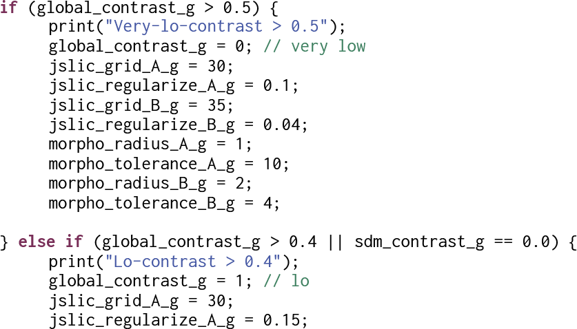

2) Perform Image Pre-processing to Adjust for Image Texture Prior to Segmentation
Depending on the Haralick IDM contrast metric stored in the global_contrast_g, we perform appropriate image pro-processing. We have found the following image pre-processing steps to be generally helpful prior to running the segmentations; however, future work remains to improve the effectiveness. ImageJ script code:

3) Compute Segmentations
Segmentations are computed for each raw, sharp, retinex, histeq, and blur image space, so features can be computed separately in each space. Depending on the desired results, we can choose which segmenter to use (jSLIC superpixels or morphological). See Figure 2.10 and note the difference between superpixel methods and morphological methods: superpixel methods produce more uniformly sized regions, while morphological methods produce a sider range of segmented region sizes.
It should be noted that segmentation region size is important, since some metrics computed over large regions can be denser than metrics computed over smaller regions which tend to be sparser. We use a range of normalization methods and other specialized algorithms to compute and compare the metrics with region size in mind, as explained in subsequent chapters where we describe each metric.
A fruitful area for future research planned for subsequent versions of the VGM is to provide more segmentations, as well as dynamic segmentations of particular regions using a range of segmentation types and parameters across (1) multiple color spaces and (2) multiple LGN pre-processed images. Using multiple segmentations as described will increase accuracy based on current test results. Because multiple segmentations will result in more genomes and more metrics processing, the increased compute load points to the need for dedicated hardware for segmentation, or least software optimized segmentation algorithms.
Here is some sample ImageJ script code used to run each segmenter.


Processing Pipeline Output Files and Unique IDs
Each segmenter outputs a master segmentation file, which we process to split up the segmented image into separate files—one file per segmented region as shown in Figure 2.11. Each genome region file name incorporates the coordinates and bounding box and the type of segmenter used. We refer to each segment as a visual genome.

As shown in Figure 2.11, segmentations are contained RGB pixel regions surrounded by a 0x00 black mask area—the mask delineates the boundary of the genome region in the bounding box. When the segmentation completes, each segmented pixel region is named using a unique 64-bit ID for the image and another ID for the genome region within the image. Genome IDs are unsigned 64-bit numbers such as 0x9100910ed407c200. For example, a metrics file is composed of two 64-bit IDs:
See Table 2.1 in the following section for a typical list of names. The 64-bit IDs provide a good amount of range.
Feature Metrics Generation
After the separate genome pixel regions are separated into files (genome_*.png))- one file for each raw, sharp, retinex, histeq, and blur space—metrics are computed from each genome file. As discussed in Chapter 4 in the “Agent Architecture” section, the sequencer controller agent computes the feature metrics for each genome, stores them in a set of metrics files, and also calls any agents registered to perform any special processing on the genome regions. A summary of the files created for each genome is shown in Table 2.1. The metrics files include all the feature metrics, the names of all the associated files, and the coordinates and size of the bounding box for each genome. Other metrics are also computed into separate files.
Details on the metrics file internal formats is provided in Chapter 5. Feature metric details are discussed separately for each color, shape, texture, and glyph feature base in Chapters 6–10.
Table 2.1: Files created for each genome
| genome_xydxdy_1524_1991_122_168__2547__jslic_RGB_maskfile___FLAG_JSLIC_F.png |
| *The bounding box image containing the genome region RGB pixels, background pixel values = 0. This file can be converted to a binary mask if needed. |
| MASTERGENOME__ 0d5107bb00680068_0ed407c200910091_RAW_IMAGE.genome.Z |
| *The 3D texture file for the RAW IMAGE genome region, contains 8,5,4,3,2 bit scale pyramid |
| MASTERGENOME__ 0d5107bb00680068_0ed407c200910091_RETINEX_IMAGE.genome.Z |
| *The 3D texture file for the RETINEX IMAGE genome region, contains 8,5,4,3,2 bit scale pyramid |
| MASTERGENOME__ 0d5107bb00680068_0ed407c200910091_SHARP_IMAGE.genome.Z |
| *The 3D texture file for the SHARP IMAGE genome region, contains 8,5,4,3,2 bit scale pyramid |
| MASTERGENOME__ 0d5107bb00680068_0ed407c200910091_BLUR_IMAGE.genome.Z |
| *The 3D texture file for the BLUR IMAGE genome region, contains 8,5,4,3,2 bit scale pyramid |
| MASTERGENOME__ 0d5107bb00680068_0ed407c200910091_HISTEQ_IMAGE.genome.Z |
| *The 3D texture file for the HISTEQ IMAGE genome region, contains 8,5,4,3,2 bit scale pyramid |
| METRICS__ 0d5107bb00680068_0ed407c200910091.metrics |
| *Cumulative metrics for the genome region, discussed in subsequent chapters. |
| AUTO_LEARNING__ 0d5107bb00680068_0f6607bb00390039.comparisonmetrics |
| *The learned ranges of acceptable values (HULL values) for each metric to determine correspondence, based on the collective metrics from the raw, retinex, sharp, and blur data, discussed in detail in Chapter 4. |
Summary
In this chapter we discuss the synthetic eye model and LGN model, which are mostly taken care of by the fine engineering found in common digital cameras and image processing library functions. We develop the concept of visual acuity on an attentional region (AR) to guide selection of a minimum segmentation region size to compose visual genomes. We define a simple model of the LGN, which include magno features for low resolution, and parvo features for full resolution. We discuss how saccadic dithering of the eye is used to increase resolution. We discuss how to automatically set up segmentation parameters and image pre-processing parameters based on image features such as texture, and discuss future work to automate segmentation and image pre-processing to emulate the eye and LGN biology. Finally, some low-level code details are provided to illustrate the model implementation.