Composite Surfaces
Tensor product Bézier patches were under development in the early 1960s; at about the same time, people started to think about piecewise surfaces. One of the first publications was de Boor’s work on bicubic splines [136] in 1962. Almost simultaneously, and apparently unaware of de Boor’s work, J. Ferguson [231] implemented piecewise bicubics at Boeing. His method was used extensively, although it had the serious flaw of using only zero corner twist vectors. An excellent account of the early industrial use of piecewise bicubics is the article by G. Peters [462].
16.1 Smoothness and Subdivision
Let x(u, v) and y(u, v) be two patches, defined over [uI–1, uI] × [vJ, vJ+1] and [uI, uI+1] × [vJ, vJ+1], respectively. They are r times continuously differentiable across their common boundary curve x(uI, v) = y(uI, v) if all u-partials up to order r agree there:
Now suppose both patches are given in Bézier form; let the control net of the “left” patch be {bij}; 0 ≤ i ≤ m, 0 ≤ j ≤ n and those of the “right” patch be {bij}; m ≤ i ≤ 2m, 0 ≤ j ≤ n. We can then invoke (14.13) for the cross boundary derivative of a Bézier patch. That formula is in local coordinates. To make the transition to global coordinates (u, v), we must invoke the chain rule:
where ΔI = uI+1 – uI. Since the ![]() are linearly independent, we may compare coefficients:
are linearly independent, we may compare coefficients:
This is the Cr condition for Bézier curves, applied to all n + 1 rows of the composite Bézier net. We thus have the Cr condition for composite Bézier surfaces: two adjacent patches are Cr across their common boundary if and only if all rows of their control net vertices can be interpreted as polygons of Cr piecewise Bézier curves. We have again succeeded in reducing a surface problem to several curve problems. The smoothness conditions apply analogously to the v-direction.
The basic theory for r = 1 is illustrated in Figure 16.1. An example of two C1 bicubic patches is shown in Figure 16.2.
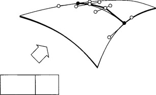
Figure 16.1 C1 continuous Bézier patches: the shown control points must be collinear and all be in the same ratio
The C1 condition states that for every j, the polygon formed by b0,j, …, b2m,j is the control polygon of a C1 piecewise Bézier curve. For this to be the case, the three points bm–1,j, bm,j,bm+1,j must be collinear and in the same ratio for all j. Simple collinearity is not sufficient: composite surfaces that have bm–1,j, bm,j,bm+1,j collinear for each j but not in the same ratio will in general not be C1. Moreover, they will not even have a continuous tangent plane. The rigidity of the C1 condition can be a serious obstacle in the design of surfaces that consist of a network of Bézier patches (or of piecewise polynomial patches in other representations).
We already saw how to use blossoms to subdidivide Bézier patches using (14.15). Here we treat an important special case more geometrically. Suppose the domain rectangle of a Bézier patch is subdivided into two subrectangles by a straight line ![]() . That line maps to an isoparametric curve on the patch, which is thus subdivided into two subpatches. We wish to find the control nets for each patch. These two patches, being part of one global surface, meet with Cn continuity. Therefore, all their rows of control points must be control polygons of Cn piecewise nth degree curves. Those curves are related to each other by the univariate subdivision process from Section 5.4.
. That line maps to an isoparametric curve on the patch, which is thus subdivided into two subpatches. We wish to find the control nets for each patch. These two patches, being part of one global surface, meet with Cn continuity. Therefore, all their rows of control points must be control polygons of Cn piecewise nth degree curves. Those curves are related to each other by the univariate subdivision process from Section 5.4.
We now have the following subdivision algorithm: interpret all rows of the control net as control polygons of Bézier curves. Subdivide each of these curves at u = û. The resulting control points form the two desired control nets. For an example, see Figure 16.3.
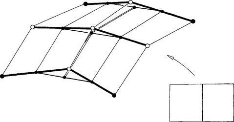
Figure 16.3 Subdivision of a Bézier patch: all rows are subdivided using the de Casteljau algorithm.
Subdivision along an isoparametric line ![]() is treated analogously. If we want to subdivide a patch into four subpatches that are generated by two isoparametric lines u = û and
is treated analogously. If we want to subdivide a patch into four subpatches that are generated by two isoparametric lines u = û and ![]() , we apply the subdivision procedure twice. It does not matter in which direction we subdivide first.
, we apply the subdivision procedure twice. It does not matter in which direction we subdivide first.
16.2 Tensor Product B-Spline Surfaces
B-spline surfaces (both rational and nonrational) play an important role in current surface design methods and will be discussed here in more detail. A parametric tensor product B-spline surface may be written as
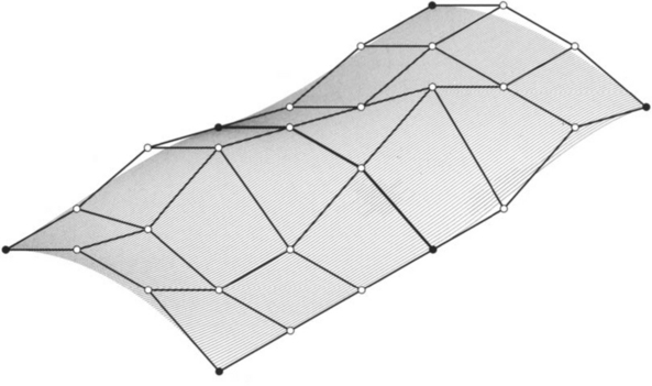
where we assume that one knot sequence in the u-direction and one in the v-direction are given. A typical bicubic surface, corresponding to triple end knots and consisting of 3 × 4 bicubic patches, is shown in Figure 16.4.
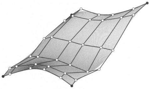
Figure 16.4 Bicubic B-spline surfaces: a surface consisting of 3 × 3 patches together with its control net.
For curves, triple end knots meant that the first and last two B-spline control points were also Bézier control points; the same is true here. The B-spline control points dij for which i or j equal 0 or 1, are also control vertices of the piecewise Bézier net of the surface. Thus they determine the boundary curves and the cross boundary derivatives.
Since a bicubic B-spline surface is a collection of bicubic patches, how can we find the Bézier net of each patch? The answer to this question may be useful for the conversion of a B-spline data format to the piecewise Bézier form. It is also relevant if we decide to evaluate a B-spline surface by first breaking it down into bicubics. The solution arises, as usual for tensor products, from the breakdown of this surface problem into a series of curve problems. If we rewrite (16.3) as
we see that for each i the sum in square brackets describes a B-spline curve in the variable u. We may convert it to Bézier form by using the univariate methods described in Chapter 8. This corresponds to interpreting the B-spline control net row by row as univariate B-spline polygons and then converting them to piecewise Bézier form. The Bézier points thus obtained may be interpreted—column by column—as B-spline polygons, which we may again transform to Bézier form one by one. This final family of Bézier polygons constitutes the piecewise Bézier net of the surface, as illustrated in Figure 16.5.
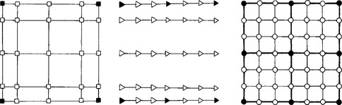
Figure 16.5 Bringing a bicubic B-spline surface into piecewise bicubic Bézier form: we first perform B-spline–Bézier curve conversion row by row, then column by column.
Needless to say, we could have started the B-spline-Bézier conversion process column by column. From the Bézier form, we may now transform to any other piecewise polynomial forms, such as the piecewise monomial or the piecewise Hermite form.
B-spline curves may be open or closed; the same is true for surfaces. Yet B-spline surfaces may be closed in two different ways: we may form surfaces with the connectivity of a cylinder or with that of a torus. No tensor product surface, however, can have the connectivity of a “double torus” or more complicated surfaces. In fact, even a surface with the topology of a sphere is not representable as a tensor product surface, at least not as one without degeneracies.
16.3 Twist Estimation
Suppose that we are given a rectangular network of points xij; 0 < I ≤ M, 0 ≤ J ≤ N and two sets of parameter values uI and vj. We want a C1 piecewise cubic surface x(u, v) that interpolates to the data points:
For a solution, we use curve methods wherever possible. We will first fit piecewise cubics to all rows and columns of data points using methods that were developed in Chapter 9. We must keep in mind, however, that all curves in the u-direction have the same parametrization, given by the uI; the v-curves are all defined over the vJ.
Creating a network of C1 (or C2) piecewise cubics through the data points is only the first step toward a surface, however. Our aim is a C1 piecewise bicubic surface, and so far we have constructed only the boundary curves for each patch. This constitutes 12 data out of the 16 needed for each patch. Figure 16.6 illustrates the situation. In Bézier form, we are still missing four interior Bézier points per patch, namely, b11, b21, b12, b22; in terms of derivatives, we must still determine the corner twists of each patch; for a definition, see Section 14.10.
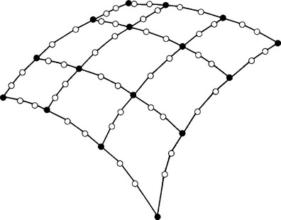
Figure 16.6 Piecewise bicubic interpolation: after a network of curves has been created, one still must determine four more coefficients per patch. A network of 3 × 3 patches is shown.
We now list a few methods to determine the missing twists.
Zero twists: Historically, this is the first twist estimation “method.” It appears, hidden in a set of formulas in pseudocode, in the paper by Ferguson [231]. Ferguson did not comment on the effects that this choice of twist vectors might have.
“Nice” surfaces exist that have identically vanishing twists—these are translational surfaces (see Figure 15.6). If the boundary curves of a patch are pairwise related by translations, then the assignment of zero twists is a good idea, but not otherwise. In these other cases, the boundary curves are not the generating curves of a translational surface. If zero twists are assigned, the generated patch will locally behave like a translational surface, giving rise to the infamous “flat spots” of zero twists. The effects of zero twists will be illustrated in Chapter 23.
If a network of patches has to be created, this choice of twists automatically guarantees C1 continuity of the overall surface. Thus it is mathematically “safe,” but does not guarantee “nice” shapes.
Adini’s twists: This method has been introduced into the CAGD literature through the paper by Barnhill, Brown, and Klucewicz [28], based on a scheme (“Adini’s rectangle”) from the finite element literature. The basic idea is this: the four cubic boundary curves define a bilinearly blended Coons patch (see Chapter 22), which happens to be a bicubic patch itself. Take the corner twists of that patch to be the desired twist vectors.
If a network of patches has to be generated, the preceding Adini’s twists would not guarantee a C1 surface. A simple modification is necessary: let four patches meet at a point, as in Figure 16.7. The four outer boundary curves of the four patches again define a bilinearly blended Coons patch. This Coons patch (consisting of four bicubics) has a well-defined twist at the parameter value where the four bicubics meet. Take that twist to be the desired twist. It is given by
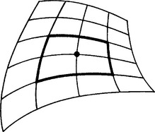
Figure 16.7 Adini’s twist: the outer boundary curves of four adjacent patches define a Coons surface; its twist at the “middle” point is Adini’s twist.
It is easy to check that Adini’s method, applied to patch boundaries of a translational surface, yields zero twists, which is desirable for that situation. Adini’s twist is a reasonable choice because, considered as an interpolant, it reproduces all bivariate polynomials of the form uvj, uiv; i,j ∈ {0, 1, 2, 3}, which is a surprisingly large set.1
Figure 16.8 compares zero twists and Adini’s twists if only one patch is used. The zero twists give rise to undesirable distortions.
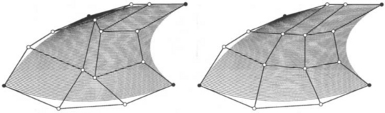
Figure 16.8 Twist estimation: the four interior Bézier points are computed to yield zero corner twists (left), and then according to Adini’s method (right).
Bessel twists: This method estimates the twist at x(uI, vJ) to be the twist of the biquadratic interpolant to the nine points x(uI+r, vJ+s); r, s ∈ {–1, 0, 1}. Since a biquadratic patch has a bilinear twist, Bessel’s twist is the bilinear interpolant to the twists of the four bilinear patches formed by the nine points. Those twists are given by
and Bessel’s twist can now be written
where
Other methods for twist estimation exist, including Brunet [94], Selesnick [570], Hagen and Schulze [303], and Farin and Hagen [206].
16.4 Bicubic Spline Interpolation
In Section 15.4, we saw how to fit an interpolating Bézier patch to a rectangular array of data points. In real life, this would not happen too often—rather we would use tensor product bicubic B-spline surfaces. The principles from Section 15.4 carry over for this case easily, and no new theory has to be developed.
Suppose we have (K + 1) × (L + 1) data points xij and two knot sequences u0, …, uK and v0, …, vL. Our development is illustrated in Figure 16.9. For each row of data points, we prescribe two end conditions (e.g., by specifying tangent vectors or Bézier points) and solve the univariate B-spline interpolation problem as described in Section 9.4. Since all these interpolation problems use the same tridiagonal coefficient matrix, an L – U decomposition should be performed before the row-by-row loop is entered. We thus produce the elements of the matrix D, marked by triangles in Figure 16.9.
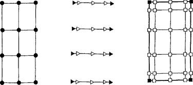
Figure 16.9 Tensor product bicubic spline interpolation: the solution is obtained in a two-step process.
We now take every column of D and perform univariate B-spline interpolation on it, again by prescribing end conditions such as clamped end tangents or Bessel tangents. The resulting control points constitute the desired B-spline control net. An example is shown in Figure 16.10. In it, the data points are connected in the u-direction—this is just to highlight the structure of the data.
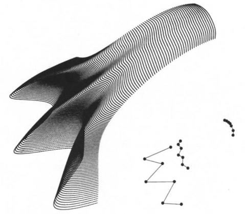
Figure 16.10 Tensor product bicubic spline interpolation: the given data, lower right (scaled down), and the solution, using Bessel end conditions and uniform parametrizations.
The final B-spline control net has two more rows and columns than X.2 This is due to the end conditions; to resolve the apparent discrepancy, we may think of X as having two additional rows and columns that constitute the end condition data. This concept is implemented in the attached code.
Although mathematically equivalent, the two processes—first row by row, then column by column; or first column by column, then row by row—do not yield the same computation count if K ≠ L.
16.5 Finding Knot Sequences
Although tensor product spline interpolation is very elegant, its use is limited to cases where the data points possess a rectangular structure. When the data points deviate from a nice grid, the problem of finding an appropriate parametrization is not easy; it may not have a solution at all. In the curve case (Section 9.6), we were able to devise several methods that assigned parameter values to the given data points. So why not take those methods and apply them to the tensor product case in much the same way in which we generalized curve methods to their tensor product counterparts? The problem is that we have to produce one set of parameter values for all isoparametric curves in the u-direction; the same holds for the v-direction.
We may endow each isoparametric curve (in the u-direction, say) with a parametrization from Section 9.6. To arrive at one parametrization for all of them, we may then carry out some averaging process. Such an approach will produce acceptable results only if all of our isoparametric curves have the same shape characteristics, that is, if they essentially yield the same parametrization. This is, however, not always the case, as Figures 16.11, 16.12, and 16.13 illustrate.3
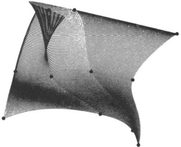
Figure 16.11 Finding knots for bicubic splines: all “horizontal” isoparametric curves have knots ui = [0, 4, 5.5, 6.0]. Note that the bottom curve has a reasonable shape.
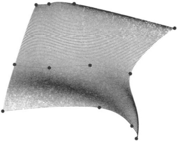
Figure 16.12 Finding knots for bicubic splines: all “horizontal” isoparametric curves have knots ui [0, 1, 2, 3].
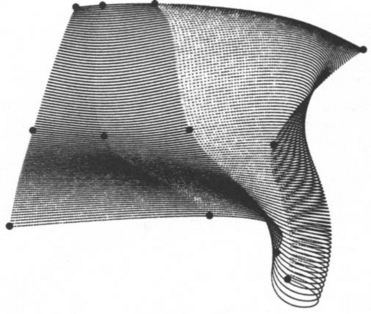
Figure 16.13 Finding knots for bicubic splines: all “horizontal” isoparametric curves have knots ui = [0, 0.5, 1.5, 6.5]. Now the top curve has a good shape.
Are there ways out of the dilemma? Not if we have unevenly distributed data and insist on bicubic spline interpolation. If we are willing to go to higher degrees and to replace C1 or C2 continuity by G1 continuity (see Chapter 20), then several methods exist; see the literature cited in that chapter.
16.6 Rational Bézier and B-Spline Surfaces
We can generalize Bézier and B-spline surfaces to their rational counterparts in much the same way as we did for the curve cases. In other words, we define a rational Bézier or B-spline surface as the projection of a 4D tensor product Bézier or B-spline surface. Thus, the rational Bézier patch takes the form
and a rational B-spline surface is written as
Figure 16.14 shows an example of a rational B-spline surface. It was obtained from the same control net as the surface in Figure 16.4, but with weights as shown in the figure. Note how the “dip” became more pronounced, as well as the “vertical ridge.”
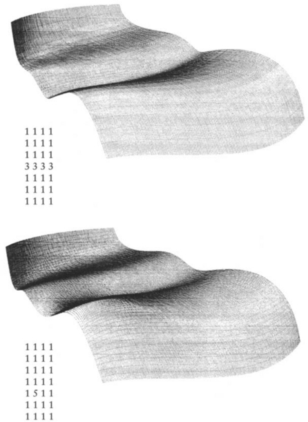
Figure 16.14 Rational B-spline surfaces: a surface together with the set of weights used to generate it.
Rational surfaces are obtained as the projections of tensor product patches, but they are not tensor product patches themselves. Recall that a tensor product surface is of the form X(u, v) = Σi Σj ci,jFi,j(u, v), where the basis functions Fi,j may be expressed as products Fi,j(u, v) = Ai(u)Bj(v). The basis functions for (16.5) are of the form
Because of the structure of the denominator, this may in general not be factored into the required form Fi,j (u, v) = Ai(u)Bj(v).
But even though rational surfaces do not possess a tensor product structure, we may use many tensor product algorithms for their manipulation. Consider, for example, the problem of finding the piecewise rational bicubic Bézier form of a rational bicubic B-spline surface. All we have to do is to convert each row of the B-spline control net into piecewise rational Bézier cubics (according to Section 13.7). Then we repeat this process for each column of the resulting net (and the resulting weights!), simply following the principle outlined in Figure 16.5.
As another example, consider the problem of extracting an isoparametric curve from a rational Bézier surface. Suppose the curve corresponds to ![]() . We simply interpret all columns of the control net as control polygons and evaluate each at
. We simply interpret all columns of the control net as control polygons and evaluate each at ![]() , using the rational de Casteljau algorithm, for example. Keep in mind that we also have to compute a weight for each control polygon. We can now interpret all obtained points together with their weights as the Bézier control polygon of the desired isoparametric curve. In general, its end weights will not be unity, that is, the curve will not be in standard form (as described in Section 13.5). This situation may be remedied by the use of the reparametrization algorithm, which is also described in that section.
, using the rational de Casteljau algorithm, for example. Keep in mind that we also have to compute a weight for each control polygon. We can now interpret all obtained points together with their weights as the Bézier control polygon of the desired isoparametric curve. In general, its end weights will not be unity, that is, the curve will not be in standard form (as described in Section 13.5). This situation may be remedied by the use of the reparametrization algorithm, which is also described in that section.
16.7 Surfaces of Revolution
Currently, rational B-spline surfaces are used for two reasons: they allow the exact representation of surfaces of revolution and of quadric surfaces. We will briefly describe surfaces of revolution in rational B-spline form here; quadric surfaces will be treated in Section 18.2.
A surface of revolution is given by
For fixed v, an isoparametric line v = const traces out a circle of radius r(v), called a meridian. Since a circle may be exactly represented by rational quadratic arcs, we may find an exact rational representation of a surface of revolution provided we can represent r(v), z(v) in rational form.
The most convenient way to define a surface of revolution is to prescribe the (planar) generating curve, or generatrix, given by
and by the axis of revolution, in the same plane as g. Suppose g is given by its control polygon, knot sequence, and weight sequence. We can construct a surface of revolution such that each meridian consists of three rational quadratic arcs, as shown in Figure 12.11. For each vertex of the generating polygon, construct an equilateral triangle (perpendicular to the axis of revolution) as in Figure 12.11. Assign the given weights of the generatrix to the three polygons corresponding to the triangle edge midpoints; assign half those weights to the three control polygons corresponding to the triangle vertices. In this way, we represent exactly “classical” surfaces such as cylinders, spheres, or tori.
Instead of breaking down each meridian into three arcs, we might have used four. The resulting four biquadratic control nets then form three concentric squares in the projection into the z = 0 plane. The control points at the squares’ midpoints are copies of the generatrix control points; their weights are those of the generatrix. The remaining weights, corresponding to the squares’ corners, are multiplied by ![]() . Figure 16.15 gives an example of a semicircle that sweeps out a surface of revolution.
. Figure 16.15 gives an example of a semicircle that sweeps out a surface of revolution.
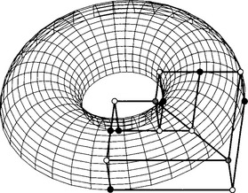
Figure 16.15 Surfaces of revolution: the surface is formed by eight rational biquadratic patches. The solid control points (shown for two patches only) have weight 1; the open points have weight 0.71, and the two gray points have weight 0.5.
Note that although the generatrix may be defined over a knot sequence {vj} with only simple knots, this is not possible for the knots of the meridian circles; we have to use double knots, thereby essentially reducing it to the piecewise Bézier form.
16.8 Volume Deformations
Sometimes local control of a surface, nice as it may be, is not what is needed. A typical design request is “stretch this surface in that direction,” or “bend that surface like so.” These are global shape deformations, and the usual tweaking of control polygon vertices is somewhat cumbersome for this task. P. Bézier devised a method to deform a Bézier patch in a manner that would satisfy this global deformation principle. We shall see that it is also applicable to B-spline surfaces. For literature, see Bézier [59], [62], [63]. A more graphics-oriented version of this principle was presented by Sederberg and Parry [558], see also [268].
To illustrate the principle, let us consider the 2D case first. Let x(t) be a planar curve (Bézier, B-spline, rational B-spline, and so forth), which is, without loss of generality, located within the (u, v) unit square. Next, let us cover the square with a regular grid of points bi,j = [i/m, j/n]T; i = 0, …, m; j = 0, …, n. We can now write every point (u, v) as
this follows from the linear precision property of Bernstein polynomials (5.14).
If we now distort the grid of bi,j into a grid ![]() , the point (u, v) will be mapped to a point
, the point (u, v) will be mapped to a point ![]() :
:
In other words, we are dealing with a mapping of ![]() .
.
In particular, the control vertices of the curve x(t) will be mapped to new control vertices, which in turn determine a new curve y(t). Note that y is only an approximation to the image of x under (16.6).4 This is highlighted by the fact that the image of x’s control polygon under (16.6) would be a collection of curve arcs, not another piecewise linear polygon.
We now have an indirect method for curve design: changing the bi,j will produce globally deformed curves. This technique may facilitate certain design tasks that are otherwise tedious to perform. Figure 16.16 gives an example of the use of this global design technique.
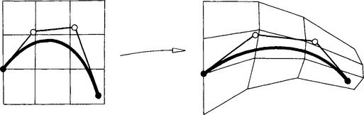
Figure 16.16 Global curve distortions: a Bézier polygon is distorted into another polygon, resulting in a deformation of the initial curve.
This technique may be generalized. For instance, we may replace the Bézier distortion (16.6) by an analogous tensor product B-spline distortion. This would reintroduce some form of local control into our design scheme.
The next level of generalization is to ![]() : we introduce a trivariate Bézier patch by
: we introduce a trivariate Bézier patch by
which constitutes a deformation of 3D space ![]() . We may use (16.7) to deform the control net of a surface embedded in the unit cube. Again, the use of a Bézier patch for the distortion is immaterial; we might have used trivariate B-splines, and so on in order to introduce some degree of locality into the method.
. We may use (16.7) to deform the control net of a surface embedded in the unit cube. Again, the use of a Bézier patch for the distortion is immaterial; we might have used trivariate B-splines, and so on in order to introduce some degree of locality into the method.
An example is shown in Figure 16.17. Part of the mushroom-shaped surface is embedded in a trivariate Bézier volume that is cubic in the vertical direction and linear in the other two. The top layer of control points is moved upward, leading to a C2 distortion of the initial object.
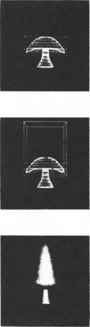
Figure 16.17 Global surface distortions: part of a surface is embedded in a Bézier volume (top). That volume is distorted (middle), leading to a distorted final object (bottom).
Why use deformation methods instead of just manipulating control vertices interactively? Volume deformation methods allow a designer to modify whole assemblies of surfaces at once, in a way that spreads out the changes in each part of the assembly in a very harmonic way. By tweaking control vertices one by one, a similarly balanced modification cannot be the result.
A practical example of volume deformations is in brain imaging. In comparative studies, many MRI brain scans have to be compared. Different people have differently shaped brains; in order to carry out a meaningful comparison, they have to be aligned (see Section 2.3); then they have to be deformed for a closer match—see [620] or [592].
16.9 CONS and Trimmed Surfaces
If we create any parametric curve (u(t), v(t)) in the domain of a surface x(u, v), it will be mapped to a curve x(u(t), v(t)) on the surface, or CONS. If the domain curve is itself a Bézier curve of degree p, then the CONS will be of degree (m + n)p, assuming m and n are the parametric degrees of x(u, v). Such curves were first considered by Bézier, see [57], [60], where they were called transposants.
In most practical applications, the curve in the domain is expressed as a piecewise linear curve, and the resulting CONS is approximated as being piecewise linear. If the piecewise linear CONS is dense enough, this should not cause problems. CONS can arise in many applications: if we intersect two surfaces, the resulting intersection curve is a CONS on either of the two surfaces. Or we could project a space curve onto a surface, again resulting in a CONS.
If the domain curve of a CONS is closed, then it divides the domain into two parts: those inside the curve and those outside. In the same way, the closed CONS divides the surface into two parts. If we want to know, for an arbitrary point (u, v) in the domain, if it lies inside the domain curve, take an arbitrary ray emanating from (u, v). Then count the number of its intersections with the domain curve. If it is even, (u, v) is outside, and inside otherwise; see Figure 16.18 for an illustration. For programming purposes, there are no “arbitrary” rays. Rays parallel to the u- or v-direction will typically suffice.
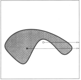
Figure 16.18 Inside/outside test: a ray from the solid point intersects the domain curve three times; it is inside. The open point is inside. The inside region is shown shaded.
CONS are mainly used for a modification of tensor product surfaces by a technique known as trimming. A trimmed surface has certain areas of it marked as invalid or invisible by a set of closed CONS. Figure 16.19 gives an example. There, two CONS are employed: one corresponds to a closed curve in the domain; the other one is the perimeter of the domain. The inside/outside test works just as it does for only one CONS.
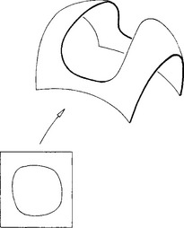
Figure 16.19 Trimmed surfaces: certain parts of a tensor product surface are marked as “invalid” by a pair of CONS.
Another example for trimmed surfaces is given in Color Plate III. Toward the lower-right quadrant of that figure, we see a small “patch” surface that blends the central part of the hood to the part over the fender. (Such surfaces, by the way, are extremely tedious to design.) If you take a close look at Color Plate III, you will see that the surfaces covered by the patch surface are not drawn where the patch surface is drawn. In fact, they are not defined there. The parts occupied by the patch surface are not part of the “regular” surfaces—they are “trimmed away.”
Trimmed surfaces should be viewed as an “engineering” extension of tensor product patches. That is to say, they are not a panacea to all surface problems either. Consider, for example, the problem of joining two trimmed surfaces in a smooth way. If they are to join along trim curves, there is no known method to ensure exact tangent plane continuity between them, as was the case for standard tensor patches. Such smoothness questions must be dealt with on a case-by-case basis, which is clearly not very desirable. Just consider the problem of fitting the aforementioned blend surface from Color Plate III between its neighbors!
Literature on trimmed surfaces: Farouki and Hinds [223], Shantz and Chang [571], Casale and Bobrow [102], Miller [427], Lasser and Bonneau [373], Brunnett [95], Vigo and Brunet [602].
16.10 Implementation
The routines in this section are written for rational surfaces. By setting all weights equal to one, the standard piecewise polynomial case is recovered.
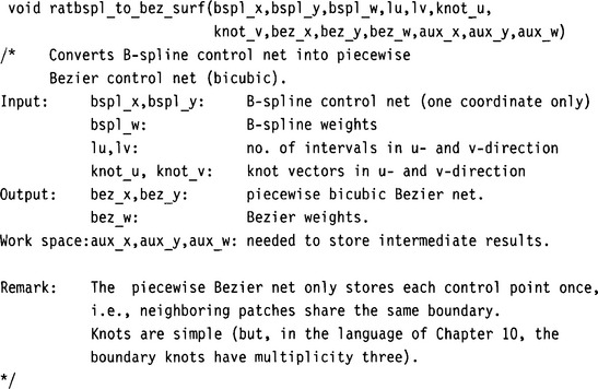
The routine that converts a rational bicubic B-spline control net into the piecewise bicubic Bézier form:
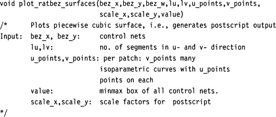
Once the piecewise rational Bézier representation of a bicubic spline surface is achieved, the following routine plots the whole surface:
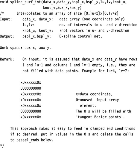
Tensor product spline interpolation (bicubic) is carried out by the following routine. It uses Bessel end conditions.
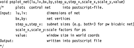
Next is the header of a program that plots the control net of a Bézier surface or of a composite surface.
16.11 Problems
1. Generalize the B-spline knot insertion algorithm to the tensor product case.
*2. Show that if two polynomial surfaces are C1 across a common boundary, then they are also twist continuous across that boundary.
*3. Suppose we want to find a parametrization {ui} for a tensor product interpolant. We may parametrize all rows of data points and then form the averages of the parametrizations thus obtained. Or we could average all rows of data points, for example, by setting ![]() and we could then parametrize the pi. Do we get the same result? Discuss both methods.
and we could then parametrize the pi. Do we get the same result? Discuss both methods.
P1. Embed your Bézier surface from Problem P3 of Chapter 14 in a tricubic grid, similar to Figure 16.17. Then “stretch” your surface, leaving the front part unchanged.
P2. Model a Klein bottle as a closed bicubic B-spline surface. Literature: [323], [170]. If you have the graphics capabilities, display your result as a translucent surface.
P3. Generate an array of points on a sphere. For latitudes, take ϕi = 0, 10, 20, …, 90 degrees. For longitudes, take ψi = 45, 50, 55, …, 75 degrees. Pass several tensor product interpolants through the data and compare their deviations from the true sphere. For the bicubic C2 spline interpolant, also compare uniform and chord length parametrizations.
1This is why this twist is called, in the context of finite elements, a serendipity element.
2This is inherited from the curve case: there one gets L + 2 control points for L data points.
3Another interesting phenomenon may be observed here: note how the first and the third of this set of surfaces have varying densities in their plots. The reason is that each cubic isoparametric curve was plotted in 90 increments on a pen plotter. With very unequal parameter spacing, this generates abruptly varying spacing on the curves.