W. Boehm
Differential Geometry II
19.1 Parametric Surfaces and Arc Element
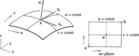
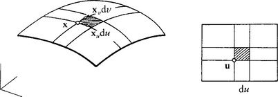
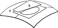
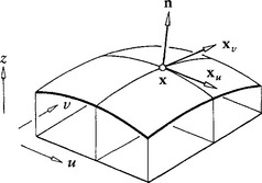
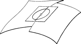
A surface may be given by an implicit form f (x, y, z) = 0 or, more useful for CAGD, by its parametric form
where the cartesian coordinates x, y, z of a surface point are differentiable functions of the parameters u and v and [a, b] denotes a rectangle in the u, v-plane; see Figure 19.1 (sometimes other domains are used, for example, triangles). To avoid potential problems with undefined normal vectors, we will assume
that is, that both families of isoparametric lines are regular (see Section 10.1) and are nowhere tangent to each other. Such a parametrization is called regular.1
Any change r = r(u) of the parameters will not change the shape of the surface; the new parametrization is regular if det[ru, rv] ≠ 0 for u ∈ [a, b], that is, if one can find the inverse u = u(r) of r.
A regular curve u = u(t) in the u, v-plane defines a regular curve x[u(t)] on the surface. One can easily compute the (squared) arc element (see Section 10.1) of this curve: from ![]() we immediately obtain
we immediately obtain
which will be written as
where
The squared arc element (19.2) is called the first fundamental form in classical differential geometry. It is of great importance for the further development of our material. Note that the arc element ds, being a geometric invariant of the curve through the point x, does not depend on the particular parametrization chosen for the representation (19.1) of the surface.
For the arc length of the surface curve defined by u = u(t), we obtain
Remark 1
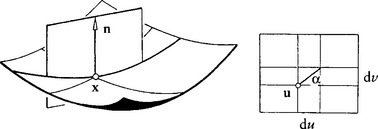
The area element corresponding to the element dudv of the u, v-plane is given by
see Figure 19.2. From ![]() a ∧ b
a ∧ b![]() 2 = a2b2 – (ab)2, we obtain
2 = a2b2 – (ab)2, we obtain
The quantity D is called the discriminant of (19.2). Thus the surface area A corresponding to a region U of the u, v-plane is given by
Remark 2
If F = 0 at a point of the surface, the two isoparametric lines that meet there are orthogonal to each other. Moreover, if F ≡ 0 at every point of the surface, the net of isoparametric lines is orthogonal everywhere.
Remark 3
Note that for any real2 du, dv, the first fundamental form ds2 is strictly positive. However, if ds2 = 0, we have two imaginary directions. These are called isotropic directions at x.
19.2 The Local Frame
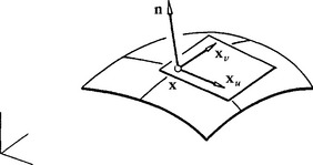
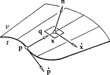
The partials xu and xv at a point x span the tangent plane to the surface at x. Let y be any point on this plane. Then
is the implicit equation of the tangent plane. The parametric equation is
The normal xu ∧ xv of the tangent plane coincides with the normal to the surface at x. The normalized normal
together with the unnormalized vectors xu, xv form a local coordinate system, a frame, at x (see Figure 19.3). This frame plays the same important role for surfaces as does the Frenet frame (see Section 10.2) for curves. The normal is of unit length and is perpendicular to xu and xv, that is, n2 = 1 and nxu = nxv, = 0. In general, the local coordinate system with origin x and axes xu, xv forms only an affine system; it is also (unlike the Frenet frame) dependent on the parametrization (19.1).
19.3 The Curvature of a Surface Curve
Let u(t) define a curve on the surface x(u). From curve theory we know that its curvature ![]() is defined by t′ = κm; the prime denotes differentiation with respect to the arc length of the curve. We will now reformulate this expression in surface terms. Since t = x′ and u′ = du/ds, v′ = dv/ds, we have
is defined by t′ = κm; the prime denotes differentiation with respect to the arc length of the curve. We will now reformulate this expression in surface terms. Since t = x′ and u′ = du/ds, v′ = dv/ds, we have
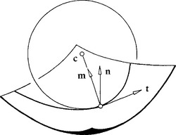
Let ϕ be the angle between the main normal m of the curve and the surface normal n at the point x under consideration, as illustrated in Figure 19.4. Then
Inserting t′ and keeping in mind that nxu = nxv = 0, we have
Furthermore, nxu = 0 implies nuxu + nxuu = 0, and so on. Thus, using the abbreviations
Eq. (19.4) can be written as
This expression is called the second fundamental form in classical differential geometry. For any given direction du/dv in the u, v-plane and any given angle ϕ, the second fundamental form, together with the first fundamental form (19.2), allows us to compute the curvature κ of a surface curve having that tangent direction.
19.4 Meusnier’s Theorem
The right-hand side of (19.4) does not contain terms involving ϕ. For ϕ = 0, that is, cos ϕ = 1, we have that m = n: the osculating plane of the curve is perpendicular to the surface tangent plane at x. The curvature κ0 of such a curve is called the normal curvature of the surface at x in the direction of t (defined by du/dv). The normal curvature is given by
Now (19.6) takes the very short form
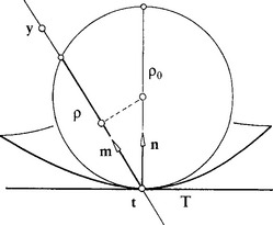
This simple formula has an interesting and important interpretation, known as Meusnier’s theorem. It is illustrated in Figure 19.5: the osculating circles of all surface curves through x having the same tangent t there form a sphere. This sphere and the surface have a common tangent plane at x; the radius of the sphere is ρ0.
As a consequence of Meusnier’s theorem, it is sufficient to study curves at x with m = n; moreover, these curves may be planar. Such curves, called normal sections, can be thought of as the intersection of the surface with a plane through x and containing n, as illustrated in Figure 19.6.
Remark 7
If the direction of the normal is chosen as in Figure 19.5, we have 0 ≤ ρ ≤ ρ0, and ρ = 0 only if ϕ = π/2, that is, if the osculating plane O coincides with the tangent plane.
19.5 Lines of Curvature
For Meusnier’s theorem, we considered (osculating) planes that contained a fixed tangent at a point on a surface; we will now look at (osculating) planes containing the normal vector at a fixed point x. We will drop the subscript of κ0 to simplify the notation.
Setting λ = dv/du = tan α (see Figure 19.6), we can rewrite (19.7) as
In the special case where L : M : N = E : F : G, the normal curvature κ is independent of λ. Points x with that property are called umbilical points.
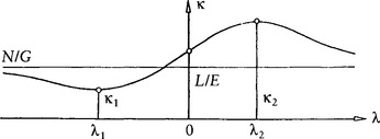
In the general case, where κ changes as λ changes, κ = κ(λ) is a rational quadratic function, as illustrated in Figure 19.7. The extreme values κ1 and κ2 of κ(λ) occur at the roots λ1 and λ2 of
It can be shown that λ1 and λ2 are always real. The extreme values κ1 and κ2 are the roots of
The quantities λ1 and λ2 define directions in the u, v-plane; the corresponding directions in the tangent plane are called principal directions. The net of lines that have these directions at all of their points is called the net of lines of curvature. If necessary, it may be constructed by integrating (19.9).
Therefore, this net of lines of curvature can be used as a parametrization of the surface; then (19.9) must be satisfied by du = 0 and by dv = 0. This implies, excluding umbilical points, that
The first equation, F ≡ 0, states that lines of curvature are orthogonal to each other; the second equation states that they are conjugate to each other as defined in Section 19.9.
At an umbilical point, the principal directions are undefined; see also Remark 9.
Remark 8
For a surface of revolution, the net of lines of curvature is defined by the meridians and the parallels; an example is shown in Figure 19.8.
19.6 Gaussian and Mean Curvature
The extreme values κ1 and κ2 of κ = κ(λ) are called principal curvatures of the surface at x. A comparison of (19.10) with κ2 – (κ1 + κ2)κ + κ1κ2 = 0 yields
and
The term K = κ1κ2 is called Gaussian curvature, whereas ![]() is called mean curvature. Note that both κ1 and κ2 change sign if the normal n is reversed, but K is not affected by such a reversal.
is called mean curvature. Note that both κ1 and κ2 change sign if the normal n is reversed, but K is not affected by such a reversal.
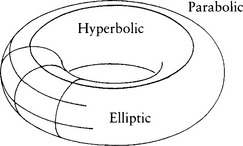
If κ1 and κ2 are of the same sign, that is, if K > 0, the point x under consideration is called elliptic. For example, all points of an ellipsoid are elliptic points. If κ1 and κ2 have different signs, that is, K < 0, the point x under consideration is called hyperbolic. For example, all points of a hyperboloid are hyperbolic points. Finally, if either κ1 = 0 or κ2 = 0, K vanishes, the point x under consideration is called parabolic. For example, all points of a cylinder are parabolic points. In the special case where both K and H vanish, one has a flat point.
The Gaussian curvature K depends on the coefficients of the first and second fundamental forms. It is a very important result, due to Gauss, that K can also be expressed only in terms of E, F, and G and their derivatives. This is known as the Theorema Egregium, which states that K depends only on the intrinsic geometry of the surface. This means it does not change if the surface is deformed in a way that does not change length measurement within it.
Remark 9
All points of a sphere are umbilic. The Gaussian and mean curvatures of a sphere are constant.
Remark 10
Any developable, that is, a surface that can be deformed to planar shape without changing length measurements in it, must have K ≡ 0. Conversely, every surface with K ≡ 0 can be developed into a plane (if necessary, by applying cuts). See also Section 19.10.
19.7 Euler’s Theorem
The normal curvatures in different directions t at a point x are not independent of each other. For simplicity, let the isoparametric curves of a surface be lines of curvature; then we have F ≡ M ≡ 0 (see Section 19.5). As a consequence, we have
and κ(λ) may be written as
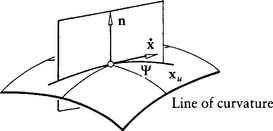
The coefficients of κ1 and κ2 have a nice geometric meaning: let Ψ denote the angle between xu and the tangent vector ![]() of the curve under consideration, as illustrated in Figure 19.9. We obtain
of the curve under consideration, as illustrated in Figure 19.9. We obtain
where ![]() as before. Hence κ(λ) may be written as
as before. Hence κ(λ) may be written as
This important result was found by L. Euler.
19.8 Dupin’s Indicatrix
Euler’s theorem has the following geometric implication. If we introduce polar coordinates ![]() and Ψ for a point y of the tangent plane at x by setting
and Ψ for a point y of the tangent plane at x by setting ![]() , then setting
, then setting ![]() Euler’s theorem can be written
Euler’s theorem can be written
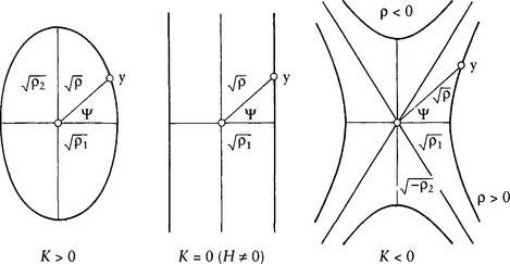
This is the equation of a conic section, the Dupin’s indicatrix (see Figure 19.10). Its points y in the direction given by Ψ have distance ![]() from x. Taking into account that a reversal of the direction of n will effect a change in the sign of ρ, this conic section is an ellipse if K > 0, a pair of hyperbolas if K < 0 (corresponding to
from x. Taking into account that a reversal of the direction of n will effect a change in the sign of ρ, this conic section is an ellipse if K > 0, a pair of hyperbolas if K < 0 (corresponding to ![]() and
and ![]() ), and a pair of parallel lines if K = 0 (but H ≠ 0).
), and a pair of parallel lines if K = 0 (but H ≠ 0).
Dupin’s indicatrix has a nice geometric interpretation: we may approximate our surface at x by a paraboloid, that is, a Taylor expansion with terms up to second order. Then Remark 7 of Chapter 10 leads to a very simple interpretation of Dupin’s indicatrix: the indicatrix, scaled down by a factor of 1 : m, can be viewed as the intersection of the surface with a plane parallel to the tangent plane at x in the distance ![]() . This is illustrated in Figure 19.11.
. This is illustrated in Figure 19.11.
Remark 11
This illustrates the appearance of a pair of hyperbolas in Figure 19.10; they appear when intersecting the surface in distances ![]() . We can thus assign a sign to the Dupin indicatrix, depending on its being “above” or “below” the tangent plane.
. We can thus assign a sign to the Dupin indicatrix, depending on its being “above” or “below” the tangent plane.
19.9 Asymptotic Lines and Conjugate Directions
The asymptotic directions of Dupin’s indicatrix have a simple geometric meaning: surface curves passing through x and having a tangent in an asymptotic direction there have zero curvature at x; in other words, these directions are defined by
They are real and different if K < 0, real but coalescing if K = 0, and complex if K > 0.
The net of lines having these directions in all of their points is called the net of asymptotic lines. If necessary, it may be calculated by integrating (19.14). In a hyperbolic region of the surface, it is real and regular and can be used for a real parametrization.
For this parametrization, one has
As earlier, let y be a point on Dupin’s indicatrix at a point x. Let ![]() denote its tangent direction at y. The direction
denote its tangent direction at y. The direction ![]() is called conjugate to the direction
is called conjugate to the direction ![]() from x to y. Consider two surface curves u1(t1) and u2(t2) that have tangent directions
from x to y. Consider two surface curves u1(t1) and u2(t2) that have tangent directions ![]() and
and ![]() at x. Some elementary calculations yield that
at x. Some elementary calculations yield that ![]() is conjugate to
is conjugate to ![]() if
if
Note that this expression is symmetric in ![]() ,
, ![]() . By definition asymptotic directions are self-conjugate.
. By definition asymptotic directions are self-conjugate.
Remark 13
The principal directions, defined by (19.9), are orthogonal and conjugate; they bisect the angles between the asymptotic directions; that is, they are the axis directions of Dupin’s indicatrix (see Figure 19.10).
Remark 14
The tangent planes of two “consecutive” points on a surface curve intersect in a straight line s. Let the curve have direction t at a point x on the surface. Then s and t are conjugate to each other. In particular, if t is an asymptotic direction, s coincides with t. If t is one of the principal directions at x, then s is orthogonal to t and vice versa. These properties characterize lines of curvature and asymptotic lines and may be used to define them geometrically.
19.10 Ruled Surfaces and Developables
If a surface contains a family of straight lines, it is called a ruled surface. It is convenient to use these straight lines as one family of isoparametric lines. Then the ruled surface may be written
where p is a point and q is a vector, both depending on t. The isoparametric lines t = const are called the generatrices of the surface; see Figure 19.12.
The partials of a ruled surface are given by ![]() and xv = q. The normal n at x is given by
and xv = q. The normal n at x is given by
A point y on the tangent plane at x satisfies
in other words, the tangent planes along a generatrix form a pencil of planes. However, if ![]() and q are linearly dependent, that is, if
and q are linearly dependent, that is, if
the tangent plane does not vary with v.
If (19.16) holds for all t, the tangent planes are fixed along each generatrix; hence all tangent planes of the surface form a one-parameter family of planes. Conversely, any one-parameter family of planes envelopes a developable surface that may be written as a ruled surface (19.15), satisfying condition (19.16); see also Remark 10.
Remark 15
The generatrices of any ruled surface coalesce with one family of its asymptotic lines. As a consequence of asymptotic lines being real, we have K ≤ 0.
Remark 16
In particular, the generatrices of a developable surface agree with its coalescing asymptotic lines, also forming one family of its lines of curvature. The second family of lines of curvature is formed by the orthogonal trajectories of the generatrices.
Remark 17
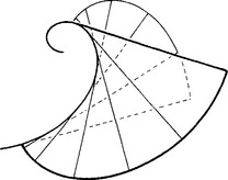
It can be shown that any developable surface is a cone p = const, a cylinder q = const, or a surface formed by all tangents of a space curve, that is, ![]() see Figure 19.13.
see Figure 19.13.
Remark 18
The normals along a line of curvature of any surface form a developable surface. This property characterizes and defines lines of curvature.
Remark 19
The tangent planes along a curve x = x[u(t)] on any surface form a developable surface. It may be developed into a plane; if by this process the curve x[u(t)] happens to be developed into a straight line, the curve x[u(t)] is called a geodesic. At any point x of a geodesic, we find that
Equation (19.17) is the differential equation of a geodesic; it is of second order. Geodesies may also be characterized as providing the shortest path between two points on the surface.
19.11 Nonparametric Surfaces
Let z = f(x, y) be a function of two variables as shown in Figure 19.14. The surface
is then called a nonparametric surface. From this, we immediately find
19.12 Composite Surfaces
A surface x = x(u, t) with global parameters u and t may be composed of patches or segments of different surfaces. Let x– = x–(t) denote the right boundary curve and x+ = x+(t) the left boundary curve of two such patches, connected along x = x(t), t ∈ [a, b], as illustrated in Figure 19.15. Both patches are tangent plane continuous if n– = ±n+ at all x(t). This may also be written
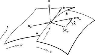
where α, β, γ are functions of t and the product αβ is nonvanishing.
The two patches are curvature continuous if they are tangent plane continuous and both Dupin’s indicatrices agree along the common boundary, in the sense of Remark 11 and as illustrated in Figure 19.16.
If the common boundary is C1, both indicatrices have a pair of points in common that are opposed to each other in the direction of the boundary tangent. Although a conic section is defined by five points (see Section 12.5), or by its midpoint and three nondiametrical points, it can be shown that both Dupin’s indicatrices coincide if there exists a family of curvature continuous surface curves crossing the common boundary. In particular, this family may be one of asymptotic lines (Pegna and Wolter [459]) or any family of isolines (Boehm [74]) or even any family of unordered directions (Pegna and Wolter [459]). Moreover, if the boundary is C0 only at a point, there are two directions of curvature continuity there, and so no further conditions have to be met.
1Examples of irregular parametrizations are shown in Figures 14.11, 14.12, and 14.13.
2Note that the vector [du, dv] defines a direction at a point x.