
Random systems are easy to understand. Consider the coin toss that starts American football games, the winner of which gets to choose to kick off or to receive the kickoff. The coin toss is not influenced by any consideration that one particular outcome might be “better” or “more entertaining” or “preferred.”
Probabilistic systems, on the other hand, consider the odds. In the card game Blackjack, the dealer for a casino hits on 16 or less and stands on 17 or more. This simple rule is based on a known long-term outcome that can be mathematically proven.
Both types of systems appear to conflict with our working definition of AI. What is the intelligent part of random? How does a fixed rule deal with changing conditions? Random decisions can simulate human behavior. Humans get bored and distracted and are subject to the urge to try something different. So an AI that is predictable will seem less intelligent than an AI that is not predictable. At the same time, an AI that randomly picks from equally good choices is just as good in the long term as an AI that picks the first of equally good choices it evaluates. Our Minesweeper AI from Chapter 4, “Rule-Based Systems,” had a very reliable figure of merit for the available choices, but it could just as easily have picked among the best choices by random selection. A similar argument can be made for FSM: Random selection is a good way to disambiguate equally good choices.
Choices are not always equally good, however. When the AI needs to avoid being predictable, it must sometimes select a sub-optimal choice. A real-life Blackjack dealer is required to be predictable; the prediction that must be true is that in the long run, the house always wins. But game AI must balance the flaw of predictability against the flaw of making sub-optimal choices. The game AI needs to consider the odds in order to strike that balance.
Odds are situational. The odds for many games of pure chance can easily be precomputed. The methods for doing so are presented in most probability and statistics books. More advanced treatments are available in books on combinatorics, which, while fascinating in its own right, might not be for the faint of heart. We will look at three ways of computing the odds: Monte Carlo methods, precomputing, and faking it. Each method has unique strengths and costs.
How can one know the odds in cases where the situation cannot be known in advance? One way is to simulate some or all of the potential game outcomes and compute the odds from the simulated results. This is known as a Monte Carlo method, and it can be directly applied to game AI. If one view of intelligence is that current actions increase future gains, then game AI could surely benefit from the ability to look into the future before making a decision.
The quality of a Monte Carlo simulation depends on how accurately the AI’s Monte Carlo simulation models the actual game situation. An AI programmer wishing to use Monte Carlo methods needs to ensure that the simulation is close enough to the situation and make sure the simulation is computationally cheap enough to be worthwhile. Also, the simulation may involve simplifications and assumptions; the programmer must ensure that they are “good enough” and that the results are better than other alternatives. Even if Monte Carlo methods are not employed, probabilistic AI needs to get the odds, also thought of as weights, to apply to the alternatives.
The accuracy of a Monte Carlo prediction depends not only on the quality of the simulation but also on how many times the simulation is run. The simulation may involve multiple points where random events, decisions, or assumptions are employed. In the case of Blackjack, a simulation may pick the next cards to be dealt using random selection from the set of cards not yet dealt. The simulation may involve deterministic decisions with random outcomes. Artillery simulations deal in the real-world concept of “circular error probable,” which means “Half the shells land inside this circle.” The more often these random points are simulated, the more likely the simulation will converge to an accurate estimation of the actual probability.
Monte Carlo methods are conceptually simple and elegant, but the development time to implement them and the computational cost to run them make them unsuitable for most game AI applications. Their narrow niche is occasional use in NPCs. An NPC that runs a simulation a few times, or only once, is impulsive or short sighted. An NPC that runs the simulation many times, however, has a very good idea of what the future holds.
Given sufficient memory, looking up the odds in a table is so much faster than any other method that it should be employed whenever possible. (“Sufficient” memory is relative; the Wii is particularly constrained for memory compared to PCs used for gaming). In many situations, the odds can be exactly precomputed. In many other situations, the odds can be approximately precomputed. There are two tricks to this. First, the approximation has to match closely enough to be useful. (Think: “This is like X, and the odds for X are....”)
The second trick is to validate the odds before the game ships. The only place to get actual numbers is from the game itself. Be warned that during development, the numbers will be change—possibly drastically—as the game evolves. Each time the game is played, it could be logging events and crunching numbers on behalf of the AI programmer. The AI programmer uses these numbers to validate the odds in the table. It is up to the AI programmer to decide if the guidance provided by any particular set of numbers should be followed. This works only if the game has the instrumentation built in early enough to generate the required amounts of data, however. There are many other benefits to building in the instrumentation as early as possible that we will not cover. Real armies need to know the circular error probable of their artillery long before they go to war; AI programmers should heed that lesson.
Known-good numbers are a great thing, but because games are an entertainment product, accurate numbers are not actually required. If the AI plays well with a warped view of its world, there is no inherent problem. The effort required to validate the actual numbers is likely to be substantial and in the long run may not be worthwhile. This brings us to our third method of getting the numbers, which is to simply fake it.
Somewhere between random selection and a good set of precomputed odds is the age-old method of faking it. The fact that experience helps is no comfort to the beginning AI programmer, but the beginner should also take heart in the fact that even experts sometimes fake it. All numbers are subject to tuning, so the sooner tuning begins, the better. Faking it means having numbers “as soon as the dart hits the dartboard,” which can happen well before the first line of instrumentation code is ever written. Usually, the first set of numbers is thought to be reasonable in some sense by the person making them up. Fewer people turn to a life of daily crime than go to a day job. What is “fewer” in actual numbers: 1 in 10? 1 in 1,000? 1 in 100,000? The numbers from current real life in a first-world country may not match the number from The Sims, and that number is probably different from Grand Theft Auto. Games are an entertainment product, so the numbers only have to be right for your game. Faking it starts by being within one or two zeroes of the final number.
For a beginner, the most serious drawback to faking it and tuning as you go is that tuning can take forever. Hard numbers (or anything close to hard numbers) place bounds on the tuning problem and guide the effort. A hybrid approach is to start by faking it as best you can. Instrumentation is designed into the game, and tuning is guided by the hard numbers as soon as they are available.
For the experienced AI programmer, faking it is actually quite liberating. Tables of numbers can be easier to tune than files of code. The AI does not have to be perfectly rational; it can think that the game world works differently than it actually does. In fact, the AI programmer can negotiate with the game designer how the game world should actually work, because that reality is just as mutable as the AI. Not only is the AI being tuned for maximum entertainment value, but so is the rest of the game world. The equations and mathematics used by experienced AI programmers to get their numbers is a book in its own right [Mark09] and will not be covered here.
With precomputed odds or a sufficient number of runs of a good simulation, the AI can accurately determine the odds of future events. The most common way such odds are used is to create weights to influence an otherwise purely random selection. The weights can take in more than the probability of success; they can also factor in potential gains, potential losses, and the cost of taking an action regardless of success or failure.
People weigh decisions this way in real life. Going to a day job each day typically has a very high probability of success, good but not great gain, almost zero potential loss, and modest costs. Buying one lottery ticket with the leftover change from a purchase has an extremely low probability of success, incredible potential gain, no potential loss, and low cost. Cutting in and out of traffic has far lower odds of success than normal driving, small potential gains in saved time, substantial potential losses from accidents and tickets, and modest additional costs in gas and wear on the car.
Impulsive behavior is easy to model with these methods. To get this with a Monte Carlo simulation, run the simulation just one time. With precomputed odds, this happens when a random selection falls outside the most probable outcomes. Much of the time, the system will select a typical response, but occasionally it will select a low-probability outcome. The normally reasonable AI is thinking, “Today is my lucky day.”
You can model compulsive behaviors by using different weights on the factors. The compulsive gambler ignores the probability of success and bases decisions on potential gains to the near exclusion of other factors. The gambler says, “I use all of my leftover money on lottery tickets.” A miser focuses on minimizing costs. “If you order a cup of hot water, you can use the free ketchup on the table to make tomato soup.” A timid person is obsessed with avoiding potential loss. “I won’t put money in the stock market or bonds, and I can barely tolerate having it in banks. Those companies could all go bankrupt!”
Slow and steady behavior weighs an accurate probability of success against potential gains, avoids unnecessary risks, and indulges lightly in cheap long-shot activities. In the real world, such people seek steady employment at a good wage, maximize their retirement contributions, carry insurance, and avoid risky behaviors, but are not above entering the occasional sweepstakes. These behaviors may lack entertainment value, but the game AI programmer benefits by knowing how to program “boring and normal.”
All the behaviors listed here can be simulated using a set of weights on the various categories. Subtle changes in the weights create richness within a category; there are a lot of different ways to be slow and steady. Gross changes in the weights yield the compulsive or near-compulsive behaviors. Games are entertainment products, so the AI programmer will need to use tools like these weights to create an interesting player experience.
If the AI problem at hand does not lend itself to numbers, probabilistic methods are of little help. Like all the other tools we have covered so far, the method forces the AI programmer to try to think of the problem in terms of this kind of solution. Some problems will have an elegant fit, and the AI programmer can orchestrate a rich variety of behaviors by changes to some numbers.
The hardest question to answer is, “Can I get the numbers?” We have covered three basic ways of getting the numbers. Sometimes a number may not tune well; it may need to be lower or higher at different times. In such cases, you replace the number with some code that computes a value based on the situation and include more numbers that will need to be tuned. The idea is to use the simplest methods that do the job and apply sophistication only as needed. (Note that this idea applies to all aspects of game AI, not just methods based on numbers.)
Probabilistic methods put a floor under artificial stupidity by coming up with reasonable actions. Random selection among best moves provides interest and removes predictability. The methods enable the AI programmer to provide a range of behaviors, including interesting or possibly baffling moves. Even good moves can be nuanced—possibly too subtly for the player to notice, but far more than we saw with FSMs. In addition, adding such nuances has a lower impact on complexity than we would see with FSMs.
There are disadvantages to these methods. The greatest is that they literally live and die on good numbers. If you cannot get those numbers, the method will fail or underperform. Not all AI programmers are comfortable with these methods, and tuning the numbers is a learned skill.
Monte Carlo methods generally are computationally expensive. If the simulation does not converge rapidly—or at all—the program will use too much CPU while delivering unreliable numbers. The simulation itself may be difficult or impossible to write. The skills and knowledge needed to write an accurate simulation can be very similar to those needed to write a regular AI in the first place. With luck, the simulation safely ignores or simplifies factors that a regular AI would be forced to deal with, but that luck is never a given.
AI systems based on numbers can drown the inexperienced AI programmer in too many numbers. If only one programmer can tune the AI, then the project is in severe difficulty if anything happens to that programmer. Extra effort is required to document what the numbers mean and how the values were derived. Games that allow user-provided content, such as mods, need to expose these numbers to a wide audience of varying skills. If those numbers are not well organized and well documented, they can be hard to deal with. This disadvantage is easily countered by experience. People who play online games are notorious for rapidly reverse-engineering the numbers and equations used in those games.
Our project is a simulation showing how different people evaluate different possible occupations and the results they get at those occupations. There are three main parts to the project: the simulation, the simulated people, and the occupations available to them. We will use four simple variables to get a wide variety of tunable behaviors. Note that while this looks like a simulation, it is only a game. It ignores all manner of social issues present in real life. Note also that the monetary system is intentionally skewed; not only does $1 mean “one day’s wages,” but some of the rest of the values are off even by that standard.
The think cycle for the AI revolves around answering the basic question, “What will this character do today?” There are many factors that will go into the answer. Because the simulation deals in money, the first important factor is how much cash the character has. The character will evaluate the available occupations based on four numbers that will have different values for each occupation. The characters do that evaluation based on their own personal equation that handles the four numbers and the amount of cash they possess in a way that fits their personalities. This equation is known variously as a fitness function or an evaluation function, and we will see it again in future chapters. Here the function can be thought of as a measure of how well each occupation fits the likes of each character.
The simulation starts a person with 10 days worth of wages in cash and runs for 1,000 work days. Each day, the simulation asks the person to pick an occupation from the seven available. This decision will be influenced by the amount of available cash and the person’s particular way of evaluating choices. The simulation will not allow the person to pick an occupation unless he or she has at least twice the cost of the particular occupation in cash. If the person picks a different job than the day before, the simulation outputs the results from the prior occupation. Then the simulation takes the selected job and randomly determines success or failure according to the odds. It deducts costs and applies gains or losses to the person’s cash. At the end of the day, the simulation deducts living expenses based on the person’s cash. The simulation brackets people as rich, doing okay, poor, and almost broke with commensurate expense levels. People who have negative cash are declared bankrupt, and their cash is mercifully reset to zero.
There are seven occupations available to our simulated people. An occupation carries a name and four items of numerical data:
The probability that the simulated person will succeed at the job on any given day, denoted as P. The probability value is given as a percent, such as 99.0 percent, but is stored as a decimal, as in 0.99.
The fixed cost of each attempt at participating in the occupation, denoted as C. This cost is spent every time the simulated person attempts the occupation, whether he or she succeeds or not.
The financial gain that the simulated player receives when he or she succeeds at an occupation. Gain is denoted as G.
The financial loss the player incurs when he or she fails an attempted occupation. The potential loss is denoted as L.
Different evaluations of these data allow the different simulated people to select occupations to their liking. These occupations include the following:
Day Job. The Day Job occupation is used as the balance point for all the others. It carries a 99 percent chance of success. The 1 percent failure rate corresponds to about 2.6 unpaid days per year. It can be thought of as, “I tried to go to work, but when I got there, work was closed.” This occupation has a gain of 1.0, which is used as the yardstick for one day’s wages. It costs 0.01 day’s wages to try to go to the day job. This attempts to factor in the cost of transportation, clothing, and other expenses that directly relate to holding down a job. There is no additional loss for failing to succeed at this occupation; the employer does not fine employees for days they do not work, it simply does not pay them.
Street. The Street occupation models begging or busking on the street and freeloading off friends. This occupation has a 75 percent chance of earning a simulated person 0.2 days’ wages, which could be thought of as 1.6 hours of pay. It has no financial downsides; the occupation is free to engage in, and there is no fee for failure.
Stunt Show. The Stunt Show occupation is hard. It has only a 70 percent chance of success. It pays handsomely at 2.5 days’ wages; the downside is that a failure costs 1.0 day’s wages. (Think of the medical bills!) Even good days have 10 times the cost of a regular job at 0.1 day’s wages, due to wear and tear on equipment.
Lotto. The Lotto occupation is not terribly promising. It has a very low chance of success, at 0.01 percent. The payoff of 10,000.0 days’ wages certainly exhibits a powerful lure, however. Playing the game costs the same amount as going to a regular job—0.01 day’s wages—and there is no additional cost for losing.
Crime. The Crime occupation succeeds 30 percent of the time and, when successful, pays an eye-opening 100 days’ wages. It is twice as expensive to do as going to a day job—a mere 0.02 day’s wages. The downside is that failure costs 200 days’ wages.
Rock Band. The Rock Band occupation has an alluring payoff of 1,000 days’ wages. It is not the same as hitting the lottery, but the 0.5 percent chance of success puts it in the reach of the dedicated artist. The lifestyle is nearly as expensive as Stunt Show at 0.05 day’s wages in direct costs. Alas, as in real life, bands that fail cannot be fined merely for being bad. No matter how much we would like it to be otherwise, there is no additional loss for failure.
Financier. The Financier occupation really pays, averaging 70 days’ wages, net, per day over the long run. It is not smooth sailing, however. Any given day has only a 66 percent chance of success, and every day has the fixed cost of 100 days’ wages. Successful days pay 220 days’ wages, and failing days cost 100 days’ wages in additional losses. A bad run of luck can be catastrophic in the short term. This attempts to model an options trader, who can lose far more than the base price of a stock. It also attempts to model the enormous profits and unlimited liability befalling a “Name” backing Lloyd’s of London throughout most of Lloyd’s history, many of whom went bankrupt in the 1990s [Wikipedia09].
The simulated people differ in exactly one regard: their method for prioritizing the occupations. In the simulation, each person provides a single equation involving the four variables that pertain to each occupation. While each person is defined in terms of a function F() of our four variables, F(P, C, G, L), we will also attempt to describe their expected behaviors in more human terms. Eddy, or “Steady Eddy,” strongly prefers a sure thing. He modulates his choices against loss but is willing to take some risks if the adjusted rewards are still high. Note the P * P terms in his equations to strongly prefer reliable gains. He ignores costs, but that does not prove to be a defect in the current implementation. As you might expect, Eddy gravitates toward the Day Job. Eddy uses the following equation to evaluate occupations:
F() = P * P * G -(1 - P)* L
Gary is a gambler. All he is after is the payoff, no matter how remote. Gary is a Lotto addict. His equation is quite simple:
F() = G
Mike is a miser. The only thing he cares about is avoiding costs. He thinks the best way to hoard money is to live on the street. His equation is also quite simple:
F() = -C
Carl is designed for a life of crime. He wants the easy big score. He does not care about potential losses or costs. His equation is as follows:
F( = P * G
Larry wants the long shot. He shoots for the big time and accepts the hardships along the way, but he has his standards about what he will and will not do. At first blush, it appears that Larry is taking the most balanced approach of all. It is interesting that he spends as much time as he can in the Rock Band occupation. This is Larry’s equation:
F( = P * G -(1 - P *L
Barry is bolder than Eddy, but he wants surer things than what Larry will attempt. He has the same P * P terms that Eddy has to prefer reliable gains. The hard knocks of the Stunt Show occupation do not deter him from the higher pay. Note the (1 —P) * (1 —P) terms that Barry uses to deemphasize potential losses; Barry thinks losses are less likely to happen to him than other people. As you might expect, his equation is very close to Eddy’s:
F( = P * P * G —(1 —P *(1 —P * L
The complexity level of this project appears to be stunningly low. An occupation has four numerical data items. Changing the values of one occupation does not affect the values of another. Adding an occupation takes exactly one short line of code. The simulated people use just one equation of those four variables, although the simulation considers cash on hand as well. Each simulated person is completely independent of any of the others. Adding or removing a person does not change the behavior of any of the others. It appears that there are almost no interactions, making the complexity growth with new additions as small as theoretically possible!
The real complexity is in the selection of those numbers and equations as a system. This system must be tuned to give pleasing results. Every added occupation could unbalance the system. You may have noticed that the simulation requires that a simulated person have twice the cost of an occupation in cash before it lets him or her select that occupation. Why twice instead of once? In testing, the Financier occupation kept wiping out people who tried it without sufficient reserves. The simulation is more pleasing with the times-two setting. The 2.5 value for Gain in Stunt Show has a very narrow band of values between spoiling Day Job and never being selected by anyone. The caution here is that tuning is required, even in a relatively simple system like this one. The good news is that the system can be tuned without heroic effort.
The people and occupations in this simulation were developed together, with each occupation aimed toward at least one particular person. When the simulation runs, the people sometimes opt for other occupations that were not explicitly tuned for their selections. These behaviors show up, or emerge, from the simulation. Emergent behaviors are a blessing and a curse. They are a blessing because they are free complex outcomes from simpler parts. They are a curse because there are no direct controls on the behaviors, and the system must be extensively tested to ensure that all such behaviors are pleasing.
The basic game is straightforward. We need to create jobs and a simulation to use them. That code will be employed by the AI we implement later so that it can act on the decisions it makes. We start with the project itself.
Launch Visual Basic.
Create a new Windows Forms Application and name it DayInTheLife.
Double-click My Project in the Solution Explorer, click the Compile tab, and set Option Strict to On. This option forces the programmer to make all type conversions explicit.
Rename Form1.vb to MainForm.vb.
Right-click DayInTheLife in the Solution Explorer, select Add → Class, and name the class Job.vb.
Add another class, named Person.vb.
Click the File menu and choose Save All.
We have all the files we need. We will hold off on the user interface until we have more of the underlying code completed.
The occupations are the easiest part of the code. The job class stores the five data items used to create it without letting outside code change them. Add the following lines of code to the class to provide storage for the data:
     'Other than the New call, this is mostly a read-only store of data.
     Private myName As String
     Private myPSuccess As Double
     Private myCost As Double
     Private myGain As Double
     Private myLoss As Double
That takes care of storage. We want the class to be created with the five values it will store. To do that, we add a New routine to the class. It will take the five values, validate them, and store them. Add the following code to the class:
     'New: store away my values
     Public Sub New(ByVal Name As String, _
             ByVal PSuccessAsPerCentage As Double, _
             ByVal Cost As Double, ByVal Gain As Double, ByVal Loss As Double)
         myName = Name
         If PSuccessAsPerCentage > 100.0 Or PSuccessAsPerCentage < 0 Then
             MsgBox("Bad PSuccess value fed to Job.New")
         End If
         'convert from percent to decimal
         myPSuccess = PSuccessAsPerCentage / 100.0
         myCost = Cost
         myGain = Gain
         myLoss = Loss
     End Sub
Having stored the five values, we need to make them available to outside code. Simple functions will do the trick. Add the following five access functions to the class:
     'Accessors to allow outside code to read our data.
     'We could have exposed them
     'as public, but we do not want them changed.

     Public Function Name() As String
         Return myName
     End Function

     'As a decimal; 99% means we return 0.99
     Public Function PSuccess() As Double
         Return myPSuccess
     End Function

     Public Function Cost() As Double
         Return myCost
     End Function

     Public Function Gain() As Double
         Return myGain
     End Function

     Public Function Loss() As Double
         Return myLoss
     End Function
There is only one thing left to do with the Job class. To make things easier, we want to be able to ask it to use a random number to compute a day’s wages or losses. To do this, we will provide the following function:
     'Return either the gain or loss
     'based on the probability.
     Public Function Wages() As Double
         If Rnd()< myPSuccess Then
             Return myGain
         Else
             Return -myLoss
         End If
     End Function
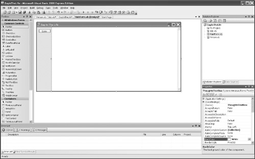
That completes the Job class. Click Save All on the File menu, and we can proceed to the user interface. Go to the Design view of MainForm.vb:
Change the Text property to Day In The Life.
Resize the form to make it larger. A size of 930 by 450 should suffice.
Drag a button to the top-left corner of the form. Change the Name property to EddyButton and the Text property to Eddy.
Drag a text box to the form. Change the Name property to Thoughts-TextBox.
Set the Multiline property to True.
Resize and position the text box to take up all of the form to the right of the Eddy button.
Set the ReadOnly property to True and the ScrollBars property to Vertical.
Set the BackColor property to White. White is available on the Web Colors tab when you click the drop-down for BackColor.
Save all.
This completes the basics of the user interface. Your screen should resemble Figure 5.1.
The name ThoughtsTextBox may be familiar from Chapter 3, “Finite State Machines.” We will reuse some of the same code in this chapter. Switch to the code for MainForm and add the following:
     'The Output side of the interface:
     Public Sub Say(ByVal someThought As String)
         'Everything we thought before, a new thought, and a newline.
         ThoughtsTextBox.AppendText(someThought & vbCrLf)
     End Sub
The MainForm will hold our occupations for the simulated people to pick from. Add the following line to the class:
Dim Occupations As New Collection
Now that we have a place to store them, we need to create our occupations. We will be intentional about which one we load first. We want the Street occupation to be the first one checked because it has a zero cost. Complete
 MainForm_Load:

         Private Sub MainForm_Load(ByVal sender As System.Object, _
                                  ByVal e As System.EventArgs) Handles MyBase.Load
             'Load the options - zero cost option must be first!
             'Format is: Occupations.Add(New Job(Name, success as %, Cost, Gain, Loss))

             'Busking/begging is free to do usually gets you almost two hours' pay
             Occupations.Add(New Job("Street", 75.0, 0.0, 0.2, 0.0))
             'Load the rest in any order.
             'Very steady way to get a full day of pay.
             Occupations.Add(New Job("Day Job", 99.0, 0.01, 1.0, 0.0))
             'This pays better but bad days hurt.
             Occupations.Add(New Job("Stuntshow", 70.0, 0.1, 2.5, 1.0))
             'Cheap with high payoff.
             Occupations.Add(New Job("Lotto", 0.01, 0.01, 10000.0, 0.0))
             'Might pay big in the short run, costs in the long run.
             Occupations.Add(New Job("Crime", 30.0, 0.02, 100.0, 200.0))
             'You play and play and one day hit it big.
             Occupations.Add(New Job("Rock band", 0.5, 0.05, 1000.0, 0.0))
             'If you can afford the costs and risks, it pays best over time.
             Occupations.Add(New Job("Financier", 66.0, 100.0, 220.0, 70.0))

             'Reseed the rnd function.
             Randomize()
         End Sub
That loads all our occupations. It also makes sure that we get different random numbers each time we run the application. Before we can go on, we need some people.
Switch to Person.vb. We will sub-class the parent class for each different person. This will make the code easy to understand. We start by working on the parent class. Add the MustInherit keyword to the class definition:
Public MustInherit Class Person
That forces us to make child classes that inherit from this parent class. The parent class will carry code that is common to all the child classes. Add the following to the class:
     'Everybody picks the same way; do it here in the parent class
     Public Function Pick(ByVal Cash As Double, _
             ByVal Occupations As Collection) As Job
         'Prime the loop
         Dim bestJob As Job = CType(Occupations(1), Job)
         Dim bestValue As Double = Me.Evaluate(bestJob, Cash)
         'Loop values:
         Dim otherJob As Job
         Dim otherValue As Double
         For Each otherJob In Occupations
             'Can I afford 2 days of this job?
             If 2.0 * otherJob.Cost <= Cash Then
                 'How much do I like it?
                 otherValue = Me.Evaluate(otherJob, Cash)
                 'More than what I have?
                 If otherValue > bestValue Then
                     bestJob = otherJob
                     bestValue = otherValue
                 End If
             End If

         Next
         Return bestJob
     End Function

     'Everybody evaluates jobs their own way.
     Public MustOverride Function Evaluate(ByVal Task As Job, _
         ByVal Cash As Double) As Double
The last line tells any child classes to provide a way to evaluate a given job. This is the member that will use the equations we developed for each person that gives a number describing how much the person likes a given job. Now we need specific people. After the End Class line, add the following code:
 'Real games would not subclass these, but it makes it simpler to understand
  Public Class Eddy
         Inherits Person
         'Eddy values a sure thing and balances loss against doubly adjusted gain.
         Public Overrides Function Evaluate(ByVal Task As Job, _
                 ByVal Cash As Double) As Double
             Return Task.PSuccess * Task.PSuccess * Task.Gain - _
                     (1 - Task.PSuccess) * Task.Loss
         End Function
     End Class
     Public Class Gary
         Inherits Person
         'Gary is all about the upside potential
         Public Overrides Function Evaluate(ByVal Task As Job, _
                     ByVal Cash As Double) As Double
             Return Task.Gain
         End Function
     End Class
     Public Class Mike
         Inherits Person
         'Mike is a miser
         Public Overrides Function Evaluate(ByVal Task As Job, _
                     ByVal Cash As Double) As Double
             Return -Task.Cost
         End Function
     End Class
     Public Class Carl
         Inherits Person
         'Carl wants easy money and doesn't care about risks
         Public Overrides Function Evaluate(ByVal Task As Job, _
                 ByVal Cash As Double) As Double
             Return Task.PSuccess * Task.Gain
         End Function
     End Class
     Public Class Larry
         Inherits Person
        'Larry is shooting for the big time but can't afford to lose
         Public Overrides Function Evaluate(ByVal Task As Job, _
                 ByVal Cash As Double) As Double
             Return Task.PSuccess * Task.Gain - (1 - Task.PSuccess) * Task.Loss
         End Function
     End Class

     Public Class Barry
         Inherits Person
        'Barry is bolder than Eddy but needs surer things than Larry
         Public Overrides Function Evaluate(ByVal Task As Job, _
                 ByVal Cash As Double) As Double
             Return Task.PSuccess * Task.PSuccess * Task.Gain - (1 - Task.PSuccess) *
     (1 - Task.PSuccess) * Task.Loss
         End Function
     End Class
It may be amazing that we can model people in just one equation of four variables. We are nearly ready to see how they respond. To do that, we must finish the simulation.
Return to the code for MainForm. We are going to add the simulation code here. The simulation will start out a person with 10 days’ wages. It will then loop through 1,000 days. Each day it will see if the person wants to change jobs. If he or she does, it will give the output from the prior job. Once a job is known, it will be evaluated for success or failure, and living expenses will be deducted. At the very end, it will show us the result of the last job held. Add the following code to the class:
     Private Sub RunSim(ByVal name As String, ByVal Dude As Person)
         ThoughtsTextBox.Clear()
         'Start with 10 days' wages.
         Dim cash As Double = 10.0
         'Fake out the curJob to get started.
         Dim curJobName As String = "Just starting out"
         Dim curJob As Job = Nothing
         'Working variables:
         Dim wages As Double
         Dim expense As Double
          'A bunch of totals to track:
          Dim daysInJob As Integer = 0
          Dim wins As Double = 0.0
          Dim losses As Double = 0.0
          Dim costs As Double = 0.0
          Dim living As Double = 0.0

          Dim i As Integer
          For i = 1 To 1000
              curJob = Dude.Pick(cash, Occupations)
              If curJob.Name < > curJobName Then
                  'Print results of last job.
                  Say(name & " spent " & daysInJob.ToString & " with job " & _
                   curJobName & " ending with $" & Format(cash, "#,##0.00") & _
                      " from $" & Format(wins, "#,##0.00") & " gains less (" & _
                      Format(losses, "#,##0.00") & " + " & _
                      Format(costs, "#,##0.00") & " + " & _
                      Format(living, "#,##0.00") & _
                      ") in losses+costs+expenses.")
                  curJobName = curJob.Name
                  daysInJob = 0
                  wins = 0.0
                  losses = 0.0
                  costs = 0.0
                  living = 0.0
              End If

              'Go to work.
              daysInJob += 1

              'Account the costs.
              cash -= curJob.Cost
              costs += curJob.Cost

              'And take the wages.
              wages = curJob.Wages
              cash += wages
              If wages > 0 Then wins += wages
              If wages < 0 Then losses -= wages

             'Do bankruptcy here.
             If cash < 0 Then
                 Debug.WriteLine("Bankruptcy")
                 cash = 0
             End If

             'Pay living expenses (free if you are broke or almost broke).
             expense = 0.0
             If cash > 500 Then
                 'Rich people spend 2.5 days' wages a day on expenses.
                 expense = 2.5
             Else
                 If cash >= 1 Then
                     'Regular people spend 25% of a day's wage to live.
                     expense = 0.25
                 Else
                     If cash >= 0.1 Then
                        'Poor people have expenses too.
                        expense = 0.025
                     End If
                 End If
             End If
             living += expense
             cash -= expense
         Next

         'Print results of last job.
         Say(name & " spent " & daysInJob.ToString & " with job " & _
             curJobName & " ending with $" & _
             Format(cash, "#,##0.00") & " from $" & _
             Format(wins, "#,##0.00") & " gains less (" & _
             Format(losses, "#,##0.00") & " + " & _
             Format(costs, "#,##0.00") & _
              " + " & Format(living, "#,##0.00") & _
              ") in losses+costs+expenses.")
     End Sub
All we need now is the code to tie the user interface to the simulation. Get to the EddyButton’s Click event handler and add the following line of code:
RunSim("Eddy", New Eddy)
We are ready to debug! Run the code and click the Eddy button a few times to see how he does. He should work steadily toward becoming a Financier, though it may take him a few tries at it. Once the code is working correctly, adding the rest of the gang is very easy:
Add a button to the form below Eddy for Larry. Larry’s event handler needs just one line of code:
RunSim("Larry", New Larry)Add a button to the form for Gary. Gary’s event handler needs this line of code:
RunSim("Gary", New Gary)Add a button to the form for Carl. Carl’s event handler needs this line of code:
RunSim("Carl", New Carl)Add a button to the form for Mike. Mike’s event handler needs this line of code:
RunSim("Mike", New Mike)Add a button to the form for Barry. Barry’s event handler needs this line of code:
RunSim("Barry", New Barry)
Run them all and see how they do. The final running project looks like Figure 5.2.
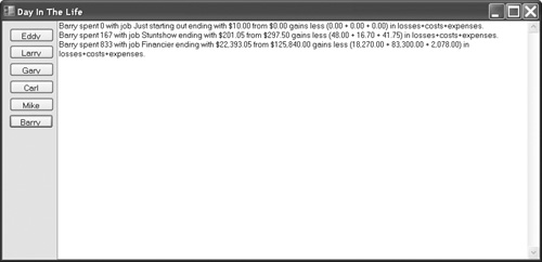
It is no surprise that Eddy works steadily at Day Job until he has saved up enough money to give Financier a try. The first few days of his new job are critical; Eddy changes jobs with only a minimal cushion against losses. Very often, he winds up back at his Day Job, possibly many times, before he takes off. It would be easy to make an interesting story of Eddy, the steady guy with a fatal flaw of reaching too soon.
Barry, less shy of losses and enamored of higher pay, follows a similar path to Larry, only faster. His Stunt Show days take him to Financier faster, but with an equally small cushion. His setbacks are shorter, and over many runs he appears to do better than Eddy. He tells a similar story.
Gary is pathetic. He gambles his money away until his habit forces him out on the street. There, he scrapes enough money to keep feeding his gambling habit until he is back on the street again. Once in a great while, he wins and retires to Lotto heaven, where the cheap cost of tickets means his winnings last him to the end.
Mike is just as pathetic. Living on the street, he saves money slowly. Alas, when he has saved a small amount, his expenses rise beyond what a street beggar can afford. Let’s face it: Even misers are averse to being hungry and cold. Our miser is not immune to spending beyond his means when he has some money saved up.
Larry just might be the most interesting character of the whole lot. He slaves away, pouring his money into his band to no avail. The costs get to him, and he can no longer keep up the lifestyle. Dejected, he spends his last few days of cash in vain on lottery tickets. This is an unexpected emergent behavior. This puts him back to playing on the street, where he saves enough to play again for a while. The cycle repeats until he hits the big-time payoff. Faced with a wad of cash, he changes careers. Unlike Eddy or Barry, Larry has enough cash to survive some initial losses as at Financier. In fact, Larry has the potential to have the highest earnings of all. No one else can get to Financier as fast as he can, and no one else does so with as big a financial cushion. Sometimes, even Larry can get wiped out in the market and go back to playing in the band. A few times, he hits it big a second time.
Carl usually spends his time failing at crime and winding up bankrupt on the street until he can scrape up enough money to try crime again. Oddly enough, sometimes he hits three successful jobs in a row. When this happens, he gives up his life of crime and takes up high-stakes finance. That often succeeds, but if it doesn’t, he can always fall back on his evil ways.
We get a great deal of mileage out of single equations of only a few variables. The code and the numbers are simple. We even get sensible unexpected behaviors out of the system.
There are clear ways to extend the simulation. Because each person is implemented as a class, we can replace the single equation with as much code as required as long as the evaluate function eventually returns sensible numbers. There could be more than one equation; there could even be a small finite state machine in there. A simpler extension would be to use the cash value directly, the number of days in job, and the day number of the simulation. The days in job number could feed wanderlust or a feeling of comfortable familiarity. The day number of the simulation could be used as a proxy for age, perhaps to adjust tolerance for risk as the person gets older.
With just a few carefully selected numbers and some finely crafted equations, you can use probability to create surprisingly realistic behaviors for game AI. Getting the numbers and equations appears deceptively easy. Tuning them is far harder.
Answers are in the appendix.