Working with Numbers and Equations
Managers and analysts routinely collect and examine key performance measures to better understand their operations and make good decisions. Being able to render the complexity of operations data into a coherent account of significant events requires an understanding of how to work well in the electronic environment with raw data.
Although some statistical and financial techniques for analyzing data are sophisticated and require specialized expertise, there are methods that are understandable and applicable by anyone with basic algebraic skills and the support of a spreadsheet package. While specialized software packages may be used in a particular business setting, Microsoft Excel is routinely available on computer desktops. Prior to renewing familiarity with the capabilities of Excel, managers should be refreshed with basic mathematical and algebraic skills to be prepared to develop a richer understanding from more advanced work.
1.1 The Magnitude of Numbers: A Quick Review
Understanding magnitudes of numbers is an important starting point. Which is greater: 0.014 or 0.01? -1.96 or -2.01? On the surface, these questions may seem trivial, but weighty decisions made in statistical terms may well rest on the appropriate comparison.
1.1.1 Evaluating Numbers by Hand
To evaluate positive numbers by hand, we align the numbers by their decimal points and then complete any digits missing to the right of the decimal with a “0,” as shown in Figure 1.1.
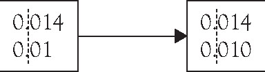
Figure 1.1. Aligning decimals at their points.
Recalling the place values of decimals shown in Figure 1.2 allows the straightforward comparison of the two numbers: 14 thousandths is larger than 10 thousandths. In mathematical notation, we can conclude that 0.014 > 0.01.
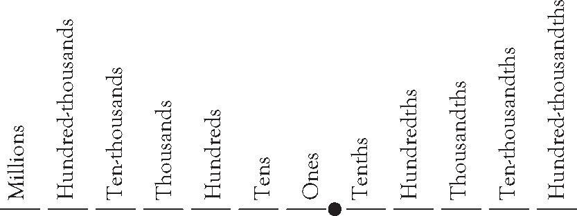
Figure 1.2. Establishing place values of decimals.
To evaluate negative numbers by hand, we may need to repeat the process shown above. In a final step, however, we need to reference a number line, remembering that smaller numbers appear to the left and larger numbers to the right, as shown in Figure 1.3. The further a value is away from zero, the more negative the value is, and the smaller that number is.
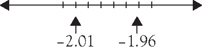
Figure 1.3. Number line comparison.
So, –2.01 falls to the left of –1.96 and is smaller than –1.96. In mathematical notation, we can conclude then that –2.01 < –1.96.
Notice in both cases that the inequality sign points to the smaller number and opens to the larger number. In fact, directional symbols and some of their meanings are shown in Table 1.1.
Table 1.1. Inequality Signs
|
Symbols |
Meaning |
|
< |
• Less than • Fewer than |
|
≤ |
• Less than or equal to • No more than |
|
> |
• Greater than • More than |
|
≥ |
• Greater than or equal to • No less than |
1.1.2 Using Excel to Evaluate Numbers
We can evaluate numbers quickly with the use of Excel. Simply type each value to be compared into a cell. Arrange the cells contiguously either in a single row or a single column. Highlight the cells containing the numbers, select “Data” and then select “Sort.” If sorted in ascending order, Excel will place the smallest number first to the greatest number last. If sorted in descending order, Excel will place the greatest number first and the smallest number last.
1.2 Order of Operations
The order in which mathematical operations are performed is significant. Different answers can be had from the same numbers and the same operations conducted in different order. For example, (3 + 1)2 is 16, but 32 + 1 is 10, and 3 + 12 is 4. We adopt common conventions to make sure we are all referring to the same procedures conducted in the same order so we can arrive at the same answers. When we deal with formulas and equations, the order of operations involved in evaluating the formula or solving the equation can be critical, whether the formulas and equations address significant financial applications or complex statistical analysis, as we will see later in this chapter.
The order in which mathematical operators are activated is:
1. Parentheses,
2. Exponents,
3. Multiply and Divide, whichever comes first left to right, and
4. Add and Subtract, whichever comes first left to right.
We have highlighted the first letters, P-E-M-D-A-S, to trigger the mnemonic device you probably learned years ago: Please Excuse My Dear Aunt Sally, capturing the order in which operations should be conducted.
1.2.1 Parentheses First
Parentheses establish priority. Information grouped within parentheses should be evaluated first. When parentheses are immediately preceded by a number, multiplication is implied. So 3 + 2 ⋅ (5 + 7) means that you add 5 and 7 first, then multiply that sum by 2, and finally add 3 to get the answer 27. If the elements grouped by parentheses are algebraic variables, as is the case in the expression 5 – 2 ⋅ (2x – 3y), where you cannot combine the terms inside the parentheses, then you must eliminate the parentheses by using the distributive property. If operations are conducted in Excel, however, a multiplication sign, indicated by the sign *, must be inserted between the number and the parentheses.
The Distributive Property of Multiplication Over Addition or Subtraction
Algebraically, when the sum of two numbers is multiplied by a third,
a ⋅ (b + c) = a ⋅ b + a ⋅ c
the multiplier a can be individually distributed to each of the numbers summed inside the parentheses, b and c.
So the expression 5 – 2 ⋅ (2x – 3y) expands with the multiplication of –2 times the binomial to achieve 5 – 4x + 6y. No further simplification is possible unless we know specific values for x and y to substitute into the expression and evaluate it. Sometimes the distributive property can be used in reverse, in a sense, to remove a common factor. For example,
597 ⋅ 439,845 + 403 ⋅ 439,845 = (597 + 403) ⋅ 439,845
= 1,000 ⋅ 439,845 = 439,845,000.
Take care with negative signs that appear in front of parentheses. If the multiplier is negative, as is the case in the expression 5 – 2 ⋅ (2x – 3y), the negative number is distributed to both terms inside the parentheses. Table 1.2 contains a quick reminder of multiplying positive and negative numbers.
Table 1.2. Multiplying Positive and Negative Numbers
|
Symbols |
Meaning |
|
+ ⋅ + = + |
A positive number times a positive number is a positive number. |
|
+ ⋅ – = – |
A positive number times a negative number is a negative number. |
|
– ⋅ + = – |
A negative number times a positive number is a negative number. |
|
– ⋅ – = + |
A negative number times a negative number is a positive number. |
So –2 ⋅ 3 = –6, but –2 ⋅ (–3) = +6. When there is just a negative sign in front of parentheses, for example – (4p + 5q), consider the expression as –1 ⋅ (4p + 5q) and use the distributive property to multiply –1 times both 4p and 5q, to yield –4p – 5q. In general, if there is an even number of negative quantities multiplied together, their product is a positive number. If there is an odd number of negative quantities multiplied together, their product is a negative number.
Occasionally, you may need to expand multiplication between the contents of two parentheses, such as (7x – 3y)(2x + 5y). Expansion of this multiplication involves, as you may recall, F-O-I-L (first-outer-inner-last), or a pattern of multiplying the first two terms, the outer two terms, the inner two terms, and the last two terms. See Figure 1.4. Finally, we combine like terms, 35xy and –6xy, to recognize the final expansion of the binomial multiplication to be 14x2 + 29xy – 15y2. Alternatively, we can expand the two binomials vertically, just like we conduct regular whole number multiplication. See Figure 1.5. Either method of expanding binomial multiplication as shown in Figure 1.4 or Figure 1.5 is acceptable.
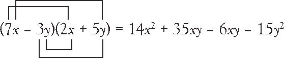
Figure 1.4. Expanding binomials horizontally using F-O-I-L.
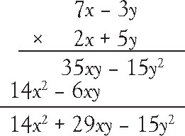
Figure 1.5. Multiplying binomials vertically.
Where parentheses occur within parentheses, begin by simplifying the inner most set first. For example, 2(5 + (3 + 1)2) = 2(5 + 42) = 2(5 + 16) = 2(21) = 42.
1.2.2 Executing Exponents
Exponents are superscripts that tally the number of times a base is multiplied. For example, 43 is 4 ⋅ 4 ⋅ 4 = 64, but 2 ⋅ 43 is 2 ⋅ 4 ⋅ 4 ⋅ 4 = 2 ⋅ 64 = 128. In applying the exponent, care must be taken to apply it only to its immediate base, and not to any preceding multiplier. If an expression combines use of both parentheses and exponents, operations within parentheses are activated first, followed by operation of the exponent: for example, (2 + 3)2 = 52 = 25 or (2 ⋅ 4)3 = 83 = 512. The expression –32 = –(32) = –3 ⋅ 3 = –9 because the negative is not part of the base, while (–3)2 = (–3) ⋅ (–3) = +9 because parentheses are used to clearly designate the base of the exponent as –3. In an algebraic expression, the same order is used to expand fm2 = f ⋅ m ⋅ m but (fm)2 = f 2 ⋅ m2. If the base of an exponent is an algebraic binomial, such as (3x – 5y)2, expansion of the binomial expression follows the example shown in Figure 1.4 or Figure 1.5: (3x – 5y) ⋅ (3x – 5y) = 9x2 – 30xy + 25y2.
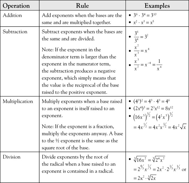
Arithmetic operations can be conducted on exponents themselves. Exponents can be added, subtracted, multiplied, or divided as shown in Table 1.3.
Table 1.3. Rules for Operations with Exponents
1.2.3 Multiply and Divide, then Add and Subtract
Continuing with the order of operations, we operate next with multiplication and division, whichever comes first left to right. So, 48 ÷ 4 ÷ 2 = 12 ÷ 2 = 6. If you operate in the wrong order, you could end up with an incorrect answer of 24. After clearing parentheses, exponents, multiplication and division, we then add and subtract from left to right. Let’s consider some examples as shown in Table 1.4.
Table 1.4. Summary Examples
|
Expression |
Steps to Solution |
Operation Used |
|
1. 4 + 6 ∙ (4 + 1) ÷ 3 – 8 = |
4 + 6 ∙ (4 + 1) ÷ 3 – 8 = |
Parentheses |
|
4 + 6 ∙ 5 ÷ 3 – 8 = |
Multiplication |
|
|
4 + 30 ÷ 3 – 8 = |
Division |
|
|
4 + 10 – 8 = |
Addition |
|
|
14 – 8 = 6 |
Subtraction |
|
|
2. 8 – 4 ÷ (5 – 3) ∙ 3 + 7 |
8 – 4 ÷ (5 – 3) ∙ 3 + 7 = |
Parentheses |
|
8 – 4 ÷ 2 ∙ 3 + 7 = |
Division |
|
|
8 – 2 ∙ 3 + 7 = |
Multiplication |
|
|
8 – 6 + 7 = |
Subtraction |
|
|
2 + 7 = 9 |
Addition |
|
|
3. 4 ∙ 8 + 12 ÷ 3 – 9 ∙ 4 |
4 ∙ 8 + 12 ÷ 3 – 9 ∙ 4 |
Multiplication |
|
32 + 12 ÷ 3 – 9 ∙ 4 |
Division |
|
|
32 + 4 – 9 ∙ 4 |
Multiplication |
|
|
32 + 4 – 36 |
Addition |
|
|
36 – 36 = 0 |
Subtraction |
|
|
4. 5 – 4 ∙ (2 + 1)2 ÷ 6 + (2 + 3)2 |
5 – 4 ∙ (2 + 1)2 ÷ 6 + (2 + 3)2 = |
Parentheses |
|
5 – 4 ∙ 32 ÷ 6 + (2 + 3)2 = |
Parentheses |
|
|
5 – 4 ∙ 32 ÷ 6 + 52 = |
Exponent |
|
|
5 – 4 ∙ 9 ÷ 6 + 52 = |
Exponent |
|
|
5 – 4 ∙ 9 ÷ 6 + 25 = |
Multiplication |
|
|
5 – 36 ÷ 6 + 25 = |
Division |
|
|
5 – 6 + 25 = |
Subtraction |
|
|
–1 + 25 = 24 |
Addition |
|
|
5. –42 |
–42 = –16 |
Exponent |
1.3 Working with Equations
Being able to carry the standard order of operations into mathematical equations and formulas is an important next step. Below we introduce some frequently used equations from statistics and finance to expand our use and understanding of the order of operations. The reason for including the equations here is primarily to practice using the order of operations contained in them with sets of data, although a brief introduction of the equation and its terms are included. Each of the equations shown, then, is presented as an opportunity for practice, not as an object that the reader should necessarily be familiar with. The solutions are shown in detail so the reader should be able to follow the calculations, step by step. The discussions following each solution focus on the issues involved to arrive at the solution using the proper order of operations. In the next section of the chapter, we review the use of Excel in working with equations.
1.3.1 Statistical Equations
The field of statistics is rich with computational equations to use in summarizing and analyzing sets of data. Working with the summation function, denoted by an upper case sigma ∑, is a skill frequently employed. The summation function works as an individual unit and requires the valuation of the sum prior to performing any surrounding operations.
Example 1.1: Sample Mean
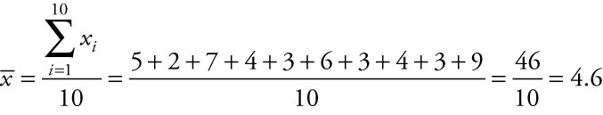
The mean is the most frequently used measure for the center of a set of data. To find a sample mean, denoted by the symbol ![]() , we sum the individual sample data values and divide by the number of observations sampled, using the equation:
, we sum the individual sample data values and divide by the number of observations sampled, using the equation:
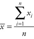
where ∑ means to sum the sampled values, xi represents each of the individual values sampled, i is an index number indicating the position the value holds in the list of individual values, and n is the number of values sampled.
The Question
A sample of debt-to-equity ratios for 10 banks shows the following values: 5%, 2%, 7%, 4%, 3%, 6%, 3%, 4%, 3%, 9%. Find the mean debt-to-equity ratio for the sample.
Answer
Using Excel
At the foot of the column or row containing the data, type: =average(range). The range represents the cells the data occupy on the spreadsheet. Alternatively, type: =sum(range), in another cell, type: =count(range), and then in a third cell, type: =(cell with sum)/(cell with count).
Discussion
The summation sign in the numerator is addressed first, because the entire numerator is divided by the denominator, 10. Once the numerator sum of 46 is obtained, we divide by 10 to find the sample mean of 4.6. The average debt-to-equity ratio for the sample is ![]() = 4.6%.
= 4.6%.
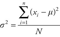
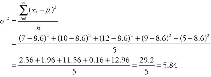
Example 1.2: Variance
The variance is a frequently used measure that describes the concentration of data around the center of a data set. For a population, the variance is denoted by the symbol σ2, pronounced sigma squared. The population variance is the sum of the squared differences of each value from its mean, m, divided by N, the number of data values in the population. To be clear, the mean for an entire population is m, whereas the mean for a sample of data selected from the population is ![]() .
.
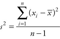
In contrast, the sample variance for a subset of data selected from a population is denoted by the symbol s2. The sample variance is the sum of the squared differences of each value from its mean, ![]() , divided by (n – 1), where the number of data values in the sample is n.
, divided by (n – 1), where the number of data values in the sample is n.
The Question
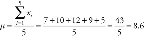
There are five departments in a school of business. The numbers of full-time professors in each of the five departments are: 7, 10, 12, 9, and 5. Find the variance among the number of full-time professors in the school.
Answer
To find the population variance among the number of full-time professors in the school, we first have to find the population mean, m, the average number of full-time professors across the five departments. The population mean is found by summing the five values and dividing by the number of departments in the school.
We then use the value of m to compute the population variance, σ2.
Using Excel
To compute the variance for the population, at the foot of the column or row containing the data, type: =varp(range). The range represents the cells the data occupy on the spreadsheet.
Discussion
Because the data given represent the entire population of departments in the school of business, we use the equation to compute the population variance, σ2. We compute the numerator first because, like the computation in Example 1.1, the entire numerator is divided by the denominator. To compute the numerator, we subtract m = 8.6 from each of the five values in the numerator. We then square each of those differences and add the squared differences together. Finally, we divide by the total number of departments, 5. The population variance for the number of full-time professors in the school of business is σ2 = 5.84.
Example 1.3: Sample Standard Deviation
The standard deviation is the positive square root of variance. For a population, the standard deviation is σ, pronounced sigma, and for a sample, the standard deviation is s.
Where the variance is given in squared units, the standard deviation is given in the same units the mean is reported in.
The Question
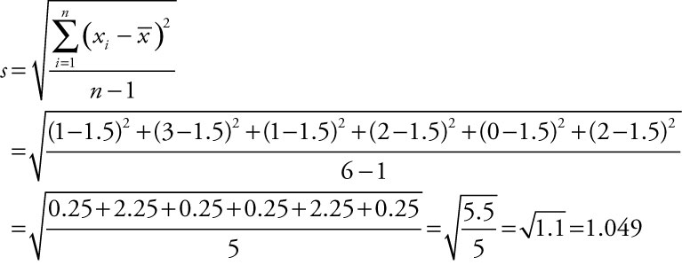
The number of knots in a sample of six boards of lumber is found to be: 1, 3, 1, 2, 0, and 2. Find the value of the sample standard deviation.
Answer
To find the sample standard deviation among the number of knots reported, we first have to find the average number of knots for the sample of boards, denoted by the symbol ![]() , using the equation:
, using the equation:
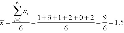
The sample standard deviation is denoted by the symbol s. To calculate the sample standard deviation, we first square the differences between each value and the mean, sum the squared differences, divide by one less than the number of boards sampled, then take the square root of our answer. When the population mean, m, is not known but is estimated by ![]() , the numerator of the calculation is divided by the sample size minus one, (n – 1). By dividing by one less than the sample size, we allow for more fluctuation in small samples to recognize potential error in using
, the numerator of the calculation is divided by the sample size minus one, (n – 1). By dividing by one less than the sample size, we allow for more fluctuation in small samples to recognize potential error in using ![]() to estimate m.
to estimate m.
Using Excel
At the foot of the column or row containing the data, type: =stdev(range). The range represents the cells that are occupied by the data on the spreadsheet.
Discussion
We compute the numerator first because the entire numerator is divided by the denominator. To compute the numerator, we take each of the six values and subtract the sample mean of 1.5 from each. We then square each of those differences and add the squared differences together. We divide by one less than the number of boards inspected, 6 – 1 or 5. Finally, we take the square root of our answer. The sample standard deviation is approximately s = 1.049 knots for the sample of boards of lumber inspected.
Example 1.4: Estimated Sample Mean for Grouped Data
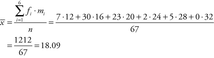
Sometimes managers may receive reports of data that have already been summarized into a frequency distribution. Alternatively, results of a study may be summarized in a publication in a way that does not include the mean. If the calculated mean is not included in the report, being able to back out an estimated mean is quite useful. For estimating either the population or the sample mean from grouped data, we use the concept of a weighted average by summing the product of the number of values in each class times the midpoint of its class as an approximation for the sum of all individual values sampled. We estimate the average miles per gallon for a sample using the equation:
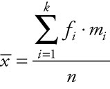
where ![]() is the estimated sample mean, fi is the frequency for each class i, mi is the midpoint for each class i, k is the number of class intervals included, and n is the number of elements sampled. The same general equation is used to estimate the population mean, m.
is the estimated sample mean, fi is the frequency for each class i, mi is the midpoint for each class i, k is the number of class intervals included, and n is the number of elements sampled. The same general equation is used to estimate the population mean, m.
The Question
Shown in Table 1.5 and Figure 1.6 are data for the miles per gallon (MPG) ratings for city driving for 67 subcompact cars for the model year 2011. Estimate the average mileage for this sample of cars.
Table 1.5. City Driving Mileages, 2011 Model US Subcompact Cars1
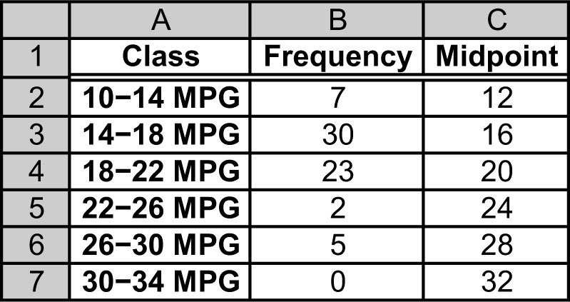
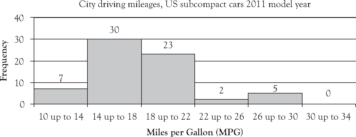
Figure 1.6. City Driving Mileages, 2011 Model US Subcompact Cars.2
Answer
Using Excel
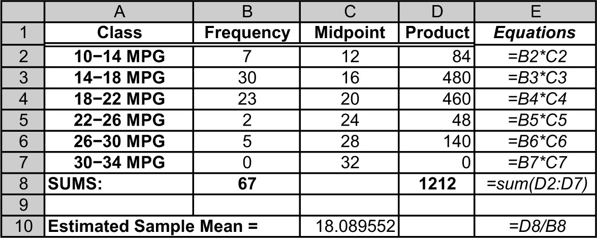
Arrange the frequency for each interval in one column and the midpoint of each interval in the adjacent column, aligned so that each interval frequency is in the same row as its midpoint. In a third column, multiply each interval’s frequency times its midpoint. Excel uses the symbol * between two values to indicate multiplication, so the products will be formed by: =(cell with frequency)*(cell with midpoint). In Table 1.6, the products in cells D2 through D7 were formed with the equations shown in cells E2 through E7. Sum the frequencies to find the value of n by typing: =sum(range), as shown in cell B8. Sum the products created by multiplying each interval’s frequency times its midpoint by typing: =sum(range), as shown in cell D8 with its equation shown in cell E8. In another cell, type: =(cell with the total of products)/(cell with sum of n), as calculated in cell C10 with its equation shown in cell E10.
Table 1.6. Using Excel to Calculate the Estimated Sample Mean3
Discussion
We compute the numerator first because the entire numerator is divided by the denominator. To compute the numerator, we multiply the frequency times the midpoint for each of the classes reported, sum across the products, and divide by the total number of elements sampled. The sample mean, ![]() , is estimated to be 18.09 miles per gallon for city driving for the sample of cars reported.
, is estimated to be 18.09 miles per gallon for city driving for the sample of cars reported.
Example 1.5: Estimated Sample Standard Deviation for Grouped Data
To estimate the sample standard deviation from grouped data, we use the class frequencies, class midpoints, and the estimated sample mean in the equation:
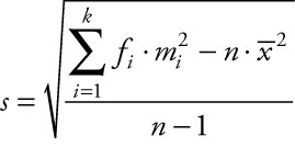
where s is the estimated sample standard deviation, fi is the frequency for each class i, mi is the midpoint for each class i, k is the number of class intervals included, and n is the number of elements included.
The Question
Compute the estimated sample standard deviation for the data presented in Example 1.4.
Answer
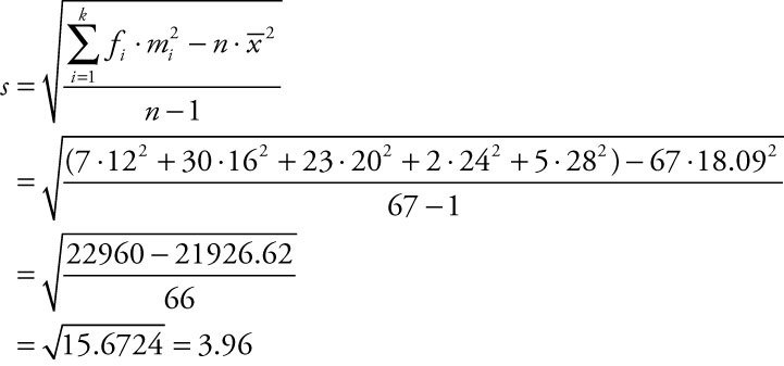
To estimate the sample standard deviation for the miles per gallon (MPG) ratings for city driving for the 67 US subcompact cars, model year 2011 included in Example 1.4, we conduct the following calculations:
Using Excel
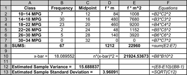
Arrange the frequency for each interval in one column and the midpoint of each interval in an adjacent column. In a third column, multiply each interval’s frequency times the square of its midpoint. Create a fourth column that contains the product of the frequency times the midpoint in cells D2 through D7. Then create a fifth column in E2 through E7 by multiplying the values in D2 through D7 by another factor of the midpoint, as shown in cells E2 through E7 in Table 1.7. In cell B8, sum the frequencies to find the value of n by typing: =sum(B2:B7). In cell D8, sum the frequencies in cells D2 through D7 by typing: =sum(D2:D7). Compute the mean in cell B10 by typing: =D8/B8. In cell E8, sum the products created by multiplying each interval’s frequency times the square of its midpoint by typing: =sum(E2:E7). That is the first component of the numerator to compute the sample variance. In cell E10, type: =B8*(B10)^2. That forms the second component of the numerator to compute the sample variance. In cell C12, type: =(E8–E10)/(B8–1). That creates the value of the estimated sample variance in cell C12. Finally in cell D13, type: =SQRT(C12), to form the estimated sample standard deviation in cell D13.
Table 1.7. Using Excel to Calculate the Estimated Sample Standard Deviation4
Discussion
We compute the summation of fm2 first, noting that the base for the exponent 2 is only the midpoint value, m, for each class; the base of the exponent does not include the class frequency, f. Also note that the right-hand term in the numerator, ![]() , is not a part of the summation because the term is preceded by the subtraction sign. We first square the midpoint values, then multiply the squared value times the frequency in each class, and add those products across the classes. Secondly, we recognize the base for the exponent 2 in the right-hand term of the numerator is only the sample mean,
, is not a part of the summation because the term is preceded by the subtraction sign. We first square the midpoint values, then multiply the squared value times the frequency in each class, and add those products across the classes. Secondly, we recognize the base for the exponent 2 in the right-hand term of the numerator is only the sample mean, ![]() . So we square the sample mean and then multiply that square by the 67 cars included in the report. We subtract the two compound values in the numerator, subtract 1 from the number of cars to form the denominator of 66, and then divide. Finally we take the square root of our answer. The estimated sample standard deviation for the city driving mileage for the 67 cars included in the report is 3.96 miles per gallon.
. So we square the sample mean and then multiply that square by the 67 cars included in the report. We subtract the two compound values in the numerator, subtract 1 from the number of cars to form the denominator of 66, and then divide. Finally we take the square root of our answer. The estimated sample standard deviation for the city driving mileage for the 67 cars included in the report is 3.96 miles per gallon.
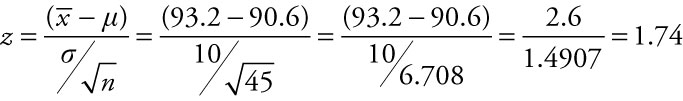
Example 1.6: The z-Score for a Sample Mean
The z-score is the scale on the axis along the bottom of the standard normal distribution. It represents the number of units of standard deviation a particular sample mean is above or below the population mean. The standard normal distribution is useful because its table details the amount of area captured under the normal curve below a given value. That area also represents the likelihood, or probability, that a value will fall within a defined segment of a normal distribution. The z-score is calculated using the equation:
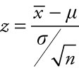
where ![]() is the sample mean, m is the population mean, σ is the population standard deviation, and n is the sample size.
is the sample mean, m is the population mean, σ is the population standard deviation, and n is the sample size.
The Question
Annual consumption of chicken in the United States is on the rise. Increasingly, it’s what’s for dinner. Population census figures place the average annual consumption of chicken at 90.6 lbs per person.5 Assuming the population standard deviation of 10 lbs in the annual consumption of chicken per capita in the United States, what is the z-score for a sample mean of 93.2 lbs of chicken consumed per person last year for a sample of 45 people in the United States?
Answer
Using Excel
In a cell, type: =(value for sample mean—value for population mean)/(value for population standard deviation/SQRT(n)).
Discussion
We begin simplifying the denominator, evaluating the square root of 45, then dividing 10 by that value. We simplify the numerator and finally divide the numerator by the denominator. The resulting z-score rounds to 1.74.
Example 1.7: Pooled Variance Estimate, Two Populations
In statistics, we use a statistical test to settle the question of whether two population means are different. Sometimes we conduct that test assuming their two variances are roughly equal. When we assume the two variances are equal, we act accordingly and combine the two sample variances to form a single pooled variance estimate, ![]() . The pooled variance estimate is calculated from the two sample variances weighted by one less than their respective sample sizes and averaged across their combined sample sizes minus two. The equation we use to combine the two sample variances is:
. The pooled variance estimate is calculated from the two sample variances weighted by one less than their respective sample sizes and averaged across their combined sample sizes minus two. The equation we use to combine the two sample variances is:
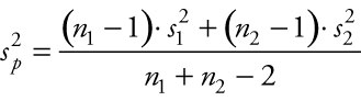
where ![]() is the pooled variance estimate, n1 is the number sampled from population 1,
is the pooled variance estimate, n1 is the number sampled from population 1, ![]() is the sample variance among the values sampled from population 1, n2 is the number sampled from population 2, and
is the sample variance among the values sampled from population 1, n2 is the number sampled from population 2, and ![]() is the sample variance among the values sampled from population 2.
is the sample variance among the values sampled from population 2.
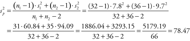
The Question
A diversified company set up separate e-commerce sites to handle orders for two of the company’s product lines. Internal auditors randomly selected 32 one-hour periods when they recorded the number of orders placed on site A and 36 periods when they recorded the number of orders placed on site B. Find the pooled variance estimate for the number of orders placed on the two sites if the variance for the first sample is 7.82 and for the second sample is 9.72.
Answer
Using Excel
Assuming the individual values for each of the two samples are available, at the foot of the two columns or rows containing the sample data, type: =count(range) for each sample. That generates the sample size for each sample. In nearby cells, type: =var(range) for each sample. In another cell, type: =(([cell with count for sample 1]–1)*[cell with variance for sample 1]+([cell with count for sample 2]–1)*[cell with variance for sample 2])/([cell with count for sample 1]+[cell with count for sample 2]–2). We will discuss some of the automated functions built into Excel’s Data Analysis Toolkit later in Chapter 3.
Discussion
We clear parentheses in the numerator, getting 31 and 35 on each term in the numerator, respectively, then square each of the two separate standard deviations. We multiply the values in each of those two terms then add the products together to form the numerator. We simplify the denominator using addition then subtraction. Finally we divide the numerator by the denominator. The pooled variance estimate for the two samples taken is 78.47.
Example 1.8: t-Score for Two Means from Populations with Equal Variances
The rationale for this example involves some complex statistical notation. The reader can skip this general introduction and still be able to evaluate the equation in terms of the order of operations performed.
The general introduction revolves around a test of two means. When we want to settle the question of whether two populations have different means, we conduct a statistical test that measures how far from zero the difference of their two means is in terms of their common standard error. If we do not know the population variances, but they are roughly equivalent, and some minimum conditions hold for the two populations, we use the two sample variances as a basis for the value of their combined standard error and evaluate a t-score using the following equation:
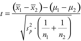
where ![]() and
and ![]() are the means from the two samples taken from populations 1 and 2, (m1 – m2) is zero because we are settling the question of whether the difference between the two means is different from zero,
are the means from the two samples taken from populations 1 and 2, (m1 – m2) is zero because we are settling the question of whether the difference between the two means is different from zero, ![]() is the pooled variance estimate shown earlier in Example 1.7, and n1 and n2 are the number of elements selected for each of the two samples. Technically, when we are settling the question of whether the difference between the two means is different from zero, we do not have to include that second term in the numerator, (m1 – m2), because it is assumed to equal zero.
is the pooled variance estimate shown earlier in Example 1.7, and n1 and n2 are the number of elements selected for each of the two samples. Technically, when we are settling the question of whether the difference between the two means is different from zero, we do not have to include that second term in the numerator, (m1 – m2), because it is assumed to equal zero.
The Question
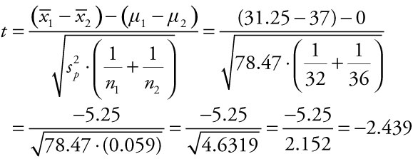
A diversified company set up separate e-commerce sites to handle orders for two of the company’s product lines. Internal auditors randomly selected 32 one-hour periods when they recorded the number of orders placed on site A and 36 periods when they recorded the number of orders placed on site B. The variance for the first sample is 7.82 and for the second sample is 9.72, and their respective sample means are 31.75 and 37. Use the pooled variance estimate of 78.47 found in Example 1.7.
Answer
Using Excel
Compute the pooled variance estimate as detailed in Example 1.7. Compute the sample means as detailed in Example 1.1. Here we assume we are looking to evaluate whether there is any difference between the two population means, which means the value of (m1 – m2) is zero. In a separate cell, type: =(cell with mean sample 1 – cell with mean sample 2)/SQRT(value of pooled variance estimate*(1/cell with count sample 1+1/cell with count sample 2)).
Discussion
Subtract the two means in the numerator. To evaluate the denominator, we start inside the parentheses by adding the two fractions. We multiply the sum of the two fractions times the value of the pooled variance estimate, then take the square root of the product. Finally, we divide the numerator by the denominator. The t-score for the difference between the two means is t = –2.439.
1.3.2 Financial Equations
While use of the summation function is prominent in many of the calculations conducted with statistical equations, the use of exponents is important in working with financial equations.
Example 1.9: Compound Interest, Future Value
To capture the effect of a lump sum of money left in an account to compound over a number of interest periods, we use the equation:
A = P(1 + i)n
where A is the future value of P dollars deposited in an account that earns i% interest in each of the n interest periods. Interest rates are often quoted on an annual basis as r% rather than the rate allocated per interest period, i%. When the interest is computed monthly,
 . When the interest is computed quarterly,
  . The time over which money accrues interest is more often quoted in years than the number of interest periods the account is active. Some adjustments may be necessary to fit the input to the equation. When the interest is computed monthly, then n = t ∙ 12. When the interest is computed quarterly, then n = t ∙ 4.
The Question
An initial deposit of $1,200 is made into an account earning 3.25% interest compounded quarterly. If the account is left to accrue interest, how much will be in the account after 5 years?
Answer
r = 0.0325, so 
t = 5 years, so n = 5 ∙ 4 = 20 interest periods
A = 1200∙(1+0.008125)20 = 1200∙1.175676 = 1410.81
Using Excel
In a cell, type: =1200*(1+0.008125)^20.
Discussion
We adjust the annual interest rate, r, to a periodic rate, i, by dividing r by 4, and we adjust the number of years, t, to the number of interest periods, n, over which the account is active by multiplying t by 4. We convert i from a percent to a decimal, add 1, and raise the sum to the nth power. That interim value, in this example $1.175676, is the future value of one dollar left in the account at i = 0.008 periodic interest rate for n = 20 interest periods. Since we began the account with $1,200, we finally multiply the initial principal times the future value of a dollar to arrive at a future value of $1,410.81 for the account.
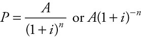
Example 1.10: Compound Interest, Present Value
If we conduct some simple algebra on the general equation contained in Example 1.9, we can solve the equation to give us what lump sum we must deposit in an account in order to have a specified value at some future date. Dividing both sides by (1 + i)n, we derive the equation:
The Question
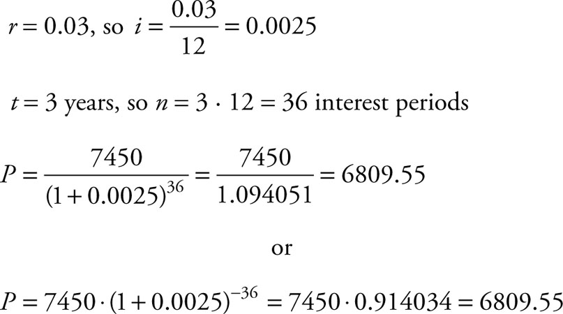
Suppose Maria has a balloon payment of $7,450 in 3 years on the new car she just leased. Unbeknownst to her, her father decides to open an account with a deposit that will cover the balloon payment at the end of her lease. If the account earns 3% compounded monthly, how much will he have to deposit in the account now to have enough to cover her balloon payment at the end of her 3-year lease?
Answer
Using Excel
In a cell, type: =7450(1+0.0025)^–36.
Discussion
The future value of a dollar invested today in an account earning 3% interest compounded monthly across 3 years is $1.094051. So we divide $7,450 by the future value to find out how many dollars we need to invest today to accrue a total of $7,450 in 3 years. Alternatively, the present value of one dollar 3 years from now is $0.914034, meaning we have to invest slightly more than $0.91 today for every dollar we want to have 3 years from now. We can multiply $7,450 times today’s value of a future dollar to determine how much we have to invest today to have $7,450 in 3 years. You will notice that
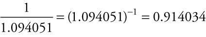
The present value of $7,450 3 years from now under 3% compounded monthly is $6,809.55, the amount her father will need to invest today to have the full amount of Maria’s balloon payment in 3 years.
Example 1.11: Effective Interest Rate
The effective interest rate is the simple interest rate that, applied to a compounding account, would yield the same interest.
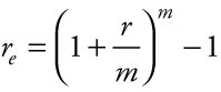
where re is the effective interest rate, r is the stated rate of interest compounding m times in a year.
The Question
Credit card accounts are an excellent environment to understand effective rates. The stated rate of interest on a credit card is 18%, but the rate is compounded every month. What is the effective interest rate?
Answer
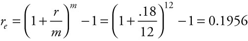
Using Excel
In a cell, type: =(1+.18/12)^12–1. In the next chapter, we review an automated function in Excel to calculate the effective interest rate.
Discussion
The equation is straightforward to compute. Inside the parentheses, we compute the periodic interest rate by dividing r by m. We then raise the sum of 1 plus the periodic interest rate to the number of interest periods in the year, and finally subtract 1. While the credit card company may advertise 18% interest on the unpaid balance, the effective interest rate is much higher, at 19.56%.
Example 1.12: Compound Interest, Future Value of an Ordinary Annuity
Examples 1.9 and 1.10 dealt with accounts that were opened with a single deposit into the account. In contrast, this example deals with a regular stream of payments made into a savings account, sometimes referred to as an annuity or a sinking fund. If the payments are made at the end of the interest period, it is called an ordinary annuity. The future value of a regular stream of payments into the account can be calculated using the equation:
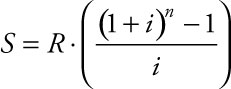
where R = the amount of the payment, i = the periodic interest rate, and n = the number of payments made.
The Question
To celebrate the birth of their daughter, Rich and Diane decided to open an account with a deposit of $25 at the end of the first month. They set up an automatic deposit so that at the end of every month, $25 is deposited into the account. The account earns 3% compounded monthly. How much will be in the account at the end of the month in which their daughter turns 21?
Answer
Adjusting the interest rate to a monthly figure yields i = 0.03/12 = 0.0025 and the time of 21 years to months yields n = 21 ∙ 12 = 252. So, over the years, Rich and Diane make 252 deposits of $25 each; they have put 252 ∙ $25 or $6,300 in principal into the account. But the account earns interest that compounds each month. Using the equation for the future value of an annuity, we find the following.
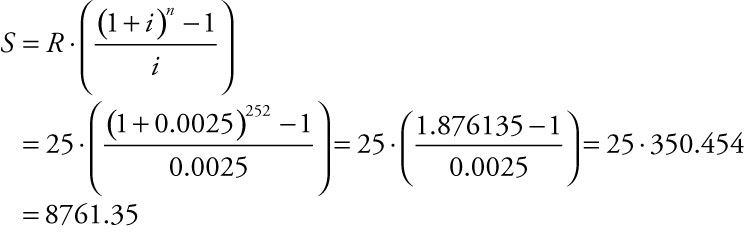
Using Excel
In a cell, type: =FV(.0025,252,–25,0,0). Alternatively, type: =25*(((1+.0025)^252–1)/.0025). In the next chapter, we review an automated function in Excel to calculate the future value of an annuity.
Discussion
Each dollar committed to a stream of 252 monthly payments earning 3% compounded monthly generates $350.454 because of the interest earned over the intervening months. Although the interest rate of 3% is low, each dollar committed is worth much more because of the number of periods over which interest compounds, nearly 40% more:
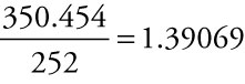
The account will be worth $8,761.35 at the end of the month in which their daughter turns 21.
Example 1.13: Present Value of an Ordinary Annuity
The present value of a stream of regular payments is appropriate when a consumer purchases an asset and pays for it over time. If the consumer takes possession of an asset now and is paying it off into the future, the lender gets the benefit of the interest, not the individual who is making the purchase. So the individual making the purchase pays the regular principal due plus interest. The present value of a regular stream of payments can be calculated using the equation:
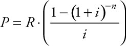
where R = the amount of the payment, i = the periodic interest rate, and n = the number of payments made.
The Question
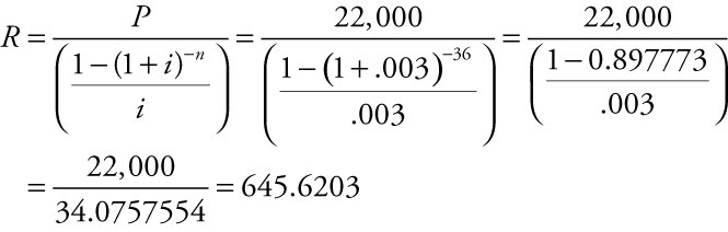
Harry decides to add a new delivery truck to his fleet. With tax and license, the truck costs $24,681.30. Harry puts $2,681.30 down and carries the rest of the cost, $22,000, on a loan that is scheduled to pay off in 3 years for 3.6% interest compounded monthly. What are his monthly payments?
Answer
Adjusting the interest rate to a monthly figure yields i = 0.036/12 = 0.003 and the time of 3 years to months yields n = 3 ∙ 12 = 36. Without calculating the cost of the interest, Harry owes $22,000 which he will pay back in 36 payments of $611.11 per payment. But Harry owes interest each month as well. To use the equation for the present value of an annuity, we need to solve for R, the monthly payment, given we know P, the amount of the loan he took out:
Using Excel
In a cell, type: =PMT(.003,36,–22000,0,0). Alternatively, in a cell, type: =22000*((1–(1+.003)^–36)/.003). In the next chapter, we review an automated function in Excel to calculate the present value of an annuity.
Discussion
The value of Harry’s monthly payment for the loan he negotiated on his truck purchase is $645.62 per month. Over the life of the loan, Harry will pay a total of $645.62 × 36 = $23,242.32, which includes ($23,242.32 – $22,000) = $1,242.32 to cover the interest due through the life of the loan.
Example 1.14: Internal Rate of Return
The internal rate of return represents the annual rate of appreciation in value from funds invested in a multi-year project. Where the other finance equations included in this chapter rely on equal payments, the internal rate of return allows for differing values to be recognized over a project’s life span. Calculations for the internal rate of return require that the same period of time be reflected in all expected costs and anticipated incomes. All other factors being equal, the project with the highest internal rate of return is comparatively preferable to projects with lower internal rates of return. The programmed Excel function =IRR(range,estimate for the rate) reflects the comparative ease with which Excel simplifies the computations.
The Question
Suppose a company is considering launching a project which they estimate will initially cost $50,000 the first year. Years 2 through 6 are projected to see revenues of $17,000; $25,000; $30,000; $32,000; and $35,000. What is the anticipated internal rate of return?
Answer
Using Excel
In an Excel spreadsheet, enter the values –50000, 17000, 25000, 30000, 32000, 35000. In a cell, type: =IRR(range,.1). Excel returns the answer to the complex calculations as 41%. Our guess of 0.1 or 10% was very low, but adequate for Excel to use as a beginning approximation of the internal rate of return.
Discussion
The internal rate of return is 41% and represents the interest rate accruing to a project that reflects both start-up costs and anticipated incomes.
Example 1.15: Net Present Value
The net present value of an investment is the present value of anticipated cash payments and cash incomes associated with a project discounted to reflect value in today’s dollars. Where the internal rate of return reports project activity as a rate of anticipated growth, the net present value reports a dollar value of the investment, the value in today’s dollar that, deposited in a bank to accrue at the projected rate, would equal the difference of payments and incomes recognized over equal periods of time.
The Question
Suppose a company is considering launching a project which they estimate will initially cost $50,000 the first year. Years 2 through 6 are projected to see revenues of $17,000; $25,000; $30,000; $32,000; and $35,000. Given an 8% discount rate, what is the net present value of this stream of activity?
Answer
Using Excel
In an Excel spreadsheet, enter the values –50000, 17000, 25000, 30000, 32000, 35000. In a cell, type: =NPV(.08,range). Excel returns the answer to the calculations as $54,009.76.
Discussion
The current value of the anticipated payments and incomes is $54,009.76, the amount one could place on deposit today earning 8% compounded annually, which at the end of 6 years, would equal the effect of the project over the next 6 years.