Chapter 5

Working with Personal Planning Over Time

We age and, over time, our incomes peak at some point. For those of us who went to work out of high school, incomes tend to peak early. For those of us who went for college or even graduate school, our incomes tend to peak later. For many of us, incomes have already peaked. The salary raise, the increased company profit, the greater rate of return are goals we strive toward but may remain elusive. Market instability, corporate vigor, job security, even personal health, may offset some of the financial advances we have made in the past. Sometimes we have to make do with less because of unforeseen developments. Taking into account various potential scenarios takes on a new level of importance in changing environments.

5.1 Retirement Planning

We plan for our golden years to remain golden, filled with sufficient gold to see us through our lives. Maintaining desired standards of living into the future in stable environments can be challenging. Let us make a few simple assumptions and develop a projection.

The Question

A couple estimates they will need $3,000 a month to supplement their Social Security benefits to maintain their current standard of living. If they retire at age 65 and anticipate living to age 90, how much should they have in the bank when they retire if we assume a constant rate of 2% annual growth compounded monthly?

Answer

The present value of a regular stream of payments can be calculated using the equation:

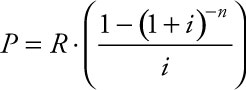
where R = the amount of the payment, i = the periodic interest rate, and n = the number of payments made. This is consistent with Example 1.13 in Chapter 1.

Table 5.1. Present Value of Monthly Payments of $R Assuming r% = 0.02 Interest Over t = 25 Years

Using Excel

The model is designed so the user enters the three values highlighted: the monthly payment, R, entered in cell B3; the annual interest rate, r, entered in cell B4; and the number of years, t, over which the payments should be funded, entered in cell B5. In cell B7, enter the equation: =B4/12. In cell B8, enter the equation: =B5*12. In cell B10, enter the equation: =B3*((1-(1+B7)^-B8)/B7), which is the equation representing the formula for the present value, P. Alternatively, in cell B10, enter the PV equation from the Insert Function: =-PV(B7,B8,B3), using cell referencing. This is consistent with Example 2.15 in Chapter 2. Entering the equation with cell references retains flexibility for the spreadsheet model, allowing the user to input a new value for the payment, the annual interest rate, the number of years, or both, and the current dollars needed to fund the stream of payments will be recalculated.

Discussion

To supplement their Social Security benefits by $3,000 a month beginning at age 65 to be drawn for 25 years to age 90, assuming a constant rate of 2% annual growth compounded monthly, the couple should have saved a total of $707,790 by age 65.

The Question

A couple estimates they will need $3,000 a month to supplement their Social Security benefits to maintain their desired standard of living. If they retire at age 65 and anticipate living to age 90 and they start saving at age 30, how much should they save each month from age 30 to age 65 to have $707,790 required to supplement their Social Security benefits by $3,000 a month, all assuming a constant rate of 2% annual growth compounded monthly?

Answer

The future value of a regular stream of payments into the account can be calculated using the equation:

where R = the amount of the payment, i = the periodic interest rate, and n = the number of payments made. This is consistent with Example 1.12 in Chapter 1.

Using Excel

The model is designed so the user enters the three values highlighted: the desired future amount, S, entered in cell B3; the annual interest rate, r, entered in cell B4; and the number of years, t, over which the payments should be funded, entered in cell B5. In cell B7, enter the equation: =B4/12. In cell B8, enter the equation: =B5*12. In cell B10, enter the equation: =B3/(((1+B7)^B8-1)/B7), which is the equation representing the formula for the monthly payment, R, needed to generate $S compounding monthly at i% over n interest periods. Alternatively, in cell B10, enter the PMT equation from the Insert Function: =-PMT(B7,B8,,B3), using cell referencing. There is a double comma in the function’s argument to indicate that the value in B3 is the future value, not the present value. This is consistent with Example 2.14 in Chapter 2. Entering the equation with cell references retains flexibility for the spreadsheet model, allowing the user to input a new value for the desired future amount, the annual interest rate, the number of years, or both, and the monthly payment needed to fund the stream of desired future value will be recalculated.

Table 5.2. Future Value of Monthly Payments of $R Assuming r% = 0.02 Interest Over t = 35 Years

Discussion

To have a total of $707,790 that is required to supplement their Social Security benefits by $3,000 a month beginning at age 65 to be drawn for 25 years to age 90, assuming a constant rate of 2% annual growth compounded monthly, the couple should save $1,165 a month between the ages of 30 and 65.

What if our hypothetical couple didn’t realize they needed to start saving for retirement until they were age 40 or even age 45? Running the same model again shows the monthly amount required to have the total of $707,790 by age 65 shoots from $1,165 a month starting to save at age 30 to $1,820 a month starting to save at age 40 and then to $2,401 a month starting to save at age 45, as shown in Table 5.3. These are easily calculated in Excel by simply changing t, the number of years in the spreadsheet model. These answers depend on stable interest rates over long periods of time, which may not be a reasonable assumption to hold. They also are made independent of any consideration of tax liability, whether funds were saved before or after taxes, all complications of the modeling that could be taken into account in a more complex modeling environment.

Table 5.3. Future Value of Monthly Payments of $R Assuming r% = 0.02 Interest Over t = 25 and 20 Years

5.2 Managing Residential Mortgages

Part of the American dream includes owning a home. Since the housing market crash of 2008, that has been more difficult to achieve. Before the market bubble burst, many homeowners refinanced their homes, sometimes with variable-rate or even interest-only mortgages that encouraged home buyers into pricier homes, the prices of which fell further once the bubble burst. Housing short sales and foreclosures have dominated the headlines, even as mortgage rates have fallen in the past few years. New home buyers, doubly cautious, spend time investigating mortgage options before venturing into the housing market. Careful management of home mortgages is important for all home owners.

The staple of home mortgages is the fixed-rate home loan. Knowing how to build an amortization schedule is an easy, but important step in managing a home loan.

Some of the expenses of owning a home can affect federal and state income taxes. Specifically, the interest expenses for home mortgages are usually deductible, which lowers one’s taxable income. Property taxes are often a deductible expense as well. So, let’s make some assumptions and investigate the impacts of interest and property tax deductions by updating our amortization schedule.

The Question

A couple plans to take out a fixed-rate home loan in the amount of $240,000 to fund the purchase of their new home. They locked in a fixed rate of 4.5% for a 30-year loan commitment. Their home is scheduled to close July 2, and the loan will fund July 1. Build an amortization schedule for their loan showing payments to interest and principal for the first 18 months of their loan.

Using Excel

Set up the headers in cells B1, B3, B4, and B5 through D5. Enter the value 240000 in cell D5. In cell A6, enter the value 1. In cell A7, enter the equation: =A6+1. Copy the equation from cell A7 down through cell A23. Highlight the block of cells B5 through D23, in the Home tab, select Cells Format, select Format Cells…, and select Currency. Click OK to format all cells in the table to show standard currency format, with a dollar sign, commas setting off the thousands place values and two places following the decimal.

The model is designed so the user enters the value highlighted: the annual interest rate, r, entered in cell B2. Enter the value 0.045 in cell B2. In cell D2, enter the equation: =B2/12. In cell B3, enter the equation: =ROUND(-PMT(B4,360,D5),2). The PMT function calculates the required payment and the ROUND function rounds the required payment to the nearest penny.

Answer

Table 5.4. Monthly Payments to Interest and Principal, r = 0.045

In cell B6, enter the equation: =ROUND(D5*D$2,2). The use of the dollar sign locks the row reference so that when the equation is copied and pasted into other cells, the cell reference to the calculated monthly interest rate remains stable. In cell C6, enter the equation: =B$3-B6. The use of the dollar sign again locks the row reference so that when the equation is copied and pasted, the monthly payment remains stable. The ROUND function makes sure the interest charge is rounded to the nearest penny so that the model agrees with calculations typically done by the lender. In cell D6, enter the equation: =D5-C6. Highlight cells B6 through D6. With your mouse, grab the lower right-hand edge of the box where the solid square appears and drag that box down through cell D23. Excel will return the calculations captured in Table 5.4.

Discussion

The couple should plan for their monthly payment to the lender to be $1,216.04. For any given monthly payment, the values shown across that row reflect the portion of their total monthly payment that goes to interest, the portion that goes toward principal, and the outstanding balance of their mortgage.

The Question

A couple plans to take out a fixed-rate home loan in the amount of $240,000 to fund the purchase of their new home. Assume the negotiated purchase price of the house was $300,000, and they plan to put $60,000 down on the home. They locked in a fixed rate of 4.5% for a 30-year loan commitment. Their home is scheduled to close July 2, and the loan will fund July 1. In addition to building an amortization schedule for their loan showing payments to interest and principal for the first 18 months of their loan, assume the couple will see 1.5% property taxes due on their purchase. To simplify the model, we will assume they will pay the property taxes due for the months of July through December in December and property taxes for the months of January through June in April of the same year. Assume the couple recognizes a combined federal and state tax rate of 30% on their incomes. Augment the amortization schedule with the cyclic payment of property taxes due each December. Finally, net the savings to their federal and state tax burdens from the mortgage and property tax payments made to produce an estimate of the real cost to them for buying the home the first year and a half.

Answer

Table 5.5. Augmented Amortization Schedule, Including Property Taxes and Income Tax Deductions

Using Excel

Augment the amortization schedule with a summary of property taxes and interest payments made during the calendar year. Year 1 includes just 6 months, so property taxes are calculated in cell F11 with the equation: =300000*0.015/2. The total interest payment made Year 1 in cell G11 is the sum of cells C6 through C11: =sum(C6:C11). To calculate the property taxes for Year 2, enter in cell F23 the equation: =300000*0.015. The total interest payment made Year 2 in cell G18 is the sum of cells C12 through C18: =sum(C12:C18). The combined interest and property income tax deductions for Year 1 in cell G14 is the sum of cell F11 plus cell G11: =F11+G11. Likewise, the combined interest and property income tax deductions for Year 2 in cell G26 is the sum of cell F23 plus cell G23: =F23+G23. The savings from income tax deductions for both years is 30% of the combined interest and property income tax deductions for each year. So, in cell G18, we include the equation: =G14*0.3; and in cell G28, we include the equation: =G26*0.3.

The net expense for holding the home Year 1 is the sum of the property tax for Year 1 in cell F11 plus 6 times the monthly mortgage payment of $1,216.04, calculated in cell C3, minus the savings from income tax deductions for Year 1 in cell G16. So in cell H17, enter the equation: =F11+6*C3-G16.

The net expense for holding the home Year 2 is the sum of the property tax for Year 2 in cell F23 plus 12 times the monthly mortgage payment of $1,216.04, calculated in cell C3, minus the savings from income tax deductions for Year 2 in cell G28. So in cell H29, enter the equation: =F23+12*C3-G28.

Discussion

Including property taxes that amount to $375 a month, funds required to cover the mortgage and the property taxes total nearly $1600 a month. But, when the deductions to the couple’s income taxes are taken into account, the real cost of owning the home in the initial years of the mortgage is just over $1,200 a month. The expense of owning a home compared to rental expense incurred in renting or leasing alternate living space should be evaluated on the real dollars of the net expense of home ownership rather than the monthly costs of the mortgage and property taxes. More complex assumptions can be factored into the expanded model to bring greater reality into the projections made here.