
Chapter 10. Working with raster data
This chapter covers
- Georeferencing with ground control points
- Working with attributes, histograms, and color tables
- Using the GDAL virtual format
- Reprojecting rasters
- Using GDAL error handling
In the last chapter you learned the basics of raster processing, such as how to read and write data and work with individual bands, and how rasters use geotransforms to orient themselves to the real world. This was a great first step, but what if you have an old aerial photograph or scanned paper map that you’d like to turn into a geographic dataset? You might want to do that because it’s fun and interesting, or you might want to do a change analysis using this data along with more current imagery. To do that, you must overlay the old data on the new. You can do this using ground control points, which are essentially a collection of points with known locations. This chapter will teach you how to use these points.
You’ll also learn how to work with raster attribute tables. Although most of the raster examples we’ve looked at so far have been continuous data, such as satellite imagery, raster datasets can also contain thematic data. In this case, each unique pixel value corresponds to a classification of some kind, such as vegetation or soil type. Pixel values are numeric, though, so how do you know what each value stands for? For example, the landcover classification map shown in figure 10.1 has 125 different classes. I certainly can’t remember what each value stands for; 76 doesn’t mean nearly as much to me as “Inter-Mountain Basins Semi-Desert Grassland” does. Fortunately, it’s possible to store information like this in raster attribute tables.
Figure 10.1. A landcover classification map, where each unique pixel value corresponds to a specific landcover classification

Note to Print Book Readers: Color Graphics
Many graphics in this book are best viewed in color. The eBook versions display the color graphics, so they should be referred to as you read. To get your free eBook in PDF, ePub, and Kindle formats, go to https://www.manning.com/books/geoprocessing-with-python to register your print book.
Take a look at figure 10.1 again. It uses a constant set of colors to display each landcover class. Water is always blue (or almost black if you’re viewing this in black and white) and the playa west of the Great Salt Lake are always a pale yellowish color (or a very light gray in black and white). Although constant colors are certainly not required for data analysis, it’s nice to have them when looking at a dataset. You saw earlier how red, green, and blue bands can be used to draw an image, but this dataset has only one band that contains classification values. Instead of the RGB bands, it has what’s called a color table that specifies what color each unique pixel value should be drawn in.
These are only a few examples of other components of raster datasets. You’ll learn how to work with these, and more, in this chapter. You’ll also learn tricks for handling errors in GDAL.
10.1. Ground control points
You’ve learned how geotransforms work to georeference an image, using the upper-left coordinates and pixel size. You don’t always have this information, however. For example, if you found an old aerial photo from 1969 and scanned it in, you’d have a digital image, but you couldn’t load it into a GIS and see it displayed in the correct location. Your scanner creates a digital image, but it doesn’t attach any sort of geographic information to it. All is not lost, however, as long as you know what area the photo is of and can identify a few locations. These locations are called ground control points (GCPs), which are points for which you know the real-world coordinates. If you can associate a number of pixels around the image with actual coordinates, then the image can be warped to overlay on a map, as shown in figure 10.2. This method isn’t used as often as geotransforms, but it’s necessary in certain cases. Plus, once an image has been georeferenced this way, a geotransform can be computed so that it can be used instead if desired. You should be aware that because the image will be stretched, warped, and/or rotated so that the GCPs overlay the real coordinates, the pixel size and raster dimensions might be changed during the process.
Figure 10.2. An example of using four known locations to warp an image to fit correctly on a map. Figure A shows an aerial photo with the points overlaid on top, figure B shows a topographical map with the same points, and figure C shows the photo stretched so that the points match up with the topo map.

It should be apparent that fixed landmarks make good GCPs because they’re the easiest thing to pinpoint and get real coordinates for. For example, if you have an aerial photograph that includes a freeway, using a car on that freeway won’t work because you probably have no way of knowing its location at the exact time the photo was taken (if you do, then by all means, use it). An exit ramp, however, is a good choice because it doesn’t move, it will be easily visible in the photo, and it’s not difficult to get the coordinates for.
Depending on the type of transformation you use to warp the image, you’ll need a different number of GCPs. One commonly used algorithm, a first-order polynomial, fits a linear equation to the image’s x coordinates so the GCP image coordinates match, as closely as possible, the real GCP coordinates that you provide. The same is done for the y coordinates. This method requires at least three points. If your coordinates are exact, then theoretically you don’t need more points, but this is probably not the case, and you’ll get better results with a few more points evenly distributed around the image. This algorithm works well if your image needs to be scaled or rotated, as in figure 10.3A. If your image needs to be bent, as in the shape changes (figure 10.3B), then you’re better off using a higher-order polynomial, such as a quadratic or cubic equation, with more GCPs.
Figure 10.3. A scaled and rotated raster (A) and a raster whose shape has changed (B)

A polynomial transformation might end up shifting several of your GCPs slightly to minimize error across the image, as in figure 10.4A. If you want to eliminate error around the GCPs and are willing to accept greater error in other parts of the image, as in figure 10.4B, you can use a spline method instead. A spline doesn’t use a single equation, but instead uses different equations for different parts of the data, so it can fit the provided points exactly. This might cause other parts of the image to be warped in odd ways, however. You can use various interpolation methods with the gdalwarp utility that comes with GDAL, but you’ll only see how to use a first-order (linear) polynomial with Python.
Figure 10.4. Different error distributions. Triangles are GCPs; circles are random points. Solid shapes are the true location; hollow shapes are the location the point ends up in the warped raster.

How do you go about using GCPs? The first things you need are the known coordinates for specific pixel offsets. You could get this information the hard way, such as opening your raster in image or photo processing software and using it to determine pixel offsets. An easier method, however, is to use the QGIS georeferencer plugin. This allows you to click on a location in your image and on an already georeferenced map, and it will tell you the pixel offsets and corresponding real-world coordinates. It will even export the necessary gdalwarp command to do the georeferencing for you. But you’re here to learn how to do the same job with Python, so let’s look at the example back in figure 10.2. This aerial photo of a small area shows a few roads and several large water treatment ponds. I’ve determined the coordinates for four locations, shown in table 10.1 and as dots in the figure. I chose points that could be identified on both the image in figure 10.2A and the topo map in figure 10.2B. Getting the point coordinates is the hard part of the process, but it’s something you’ll have to do by hand. In this case, the topo map was georeferenced so I could figure out the coordinates from the map.
Table 10.1. Pixel offsets and coordinates used to georeference the aerial photo shown in figure 10.2
|
Photo column |
Photo row |
Longitude |
Latitude |
|---|---|---|---|
| 1078 | 648 | -111.931075 | 41.745836 |
| 3531 | 295 | -111.901655 | 41.749269 |
| 3722 | 1334 | -111.899180 | 41.739882 |
| 1102 | 2548 | -111.930510 | 41.728719 |
The following listing shows how you would attach these ground control points to the photo.
Listing 10.1. Adding ground control points to a raster

When adding GCPs to a raster, make sure you open the dataset for updating, as you do here. You also need the spatial reference system of the known coordinates; in this case they use the WGS84 datum but are unprojected (lat/lon). The last thing you need is a list of GCPs, and you can create each of those with the GCP constructor shown here:
gdal.GCP([x], [y], [z], [pixel], [line], [info], [id])
- x, y, and z are the real-world coordinates corresponding to the point. All are optional and default to 0, although you probably don’t want x and y values to be 0.
- pixel is the column offset for the pixel with known coordinates. This is optional and the default is 0.
- line is the row offset for the pixel with known coordinates. This is optional and the default is 0.
- info and id are two optional strings used to identify the GCP, but in my experience they don’t carry over to the image. I rarely use GCPs, however, so perhaps there are instances where they do. The default is a blank string.
In listing 10.1 you use the information in table 10.1 to create a list of four GCPs, and then you attach those GCPs to the dataset with SetGCPs. This function requires a list of GCPs and a WKT string containing projection information for the real-world coordinates.
Now that you’ve added GCPs, software that understands them can display your image in its correct location. If you don’t need to know what GCPs were used to georeference the image and would rather use the more common geotransform method of georeferencing, you can create a geotransform from the GCPs and set that on the dataset instead of attaching the GCPs. To create a geotransform using a first-order transformation, pass your list of GCPs to GCPsToGeoTransform. Then make sure you set both the geotransform and the projection information on your dataset:
ds.SetProjection(sr.ExportToWkt())
ds.SetGeoTransform(gdal.GCPsToGeoTransform(gcps))
You don’t have to convert your GCPs to a geotransform if you don’t want to, however.
10.2. Converting pixel coordinates to another image
As you learned in the last chapter, functions can help you convert between real-world coordinates and pixel offsets. Also, a Transformer class can be used for that or to go between offsets in two different rasters. One example of why you might want to do this is if you’re mosaicking rasters together, because each input image goes in a different part of the mosaic. To illustrate this, let’s combine a few digital orthophotos of Cape Cod together into one raster.
To combine the images, it’s necessary to know the extent of the output mosaic. The only way to find this is to get the extent of each input raster and calculate the overall minimum and maximum coordinates (figure 10.5). To make this a little easier, you’ll create a function that gets the extent of a raster. It uses the geotransform to get the upper-left coordinates and then calculates the lower right coordinates using the pixel size and raster dimensions:
def get_extent(fn):
    '''Returns min_x, max_y, max_x, min_y'''
    ds = gdal.Open(fn)
    gt = ds.GetGeoTransform()
    return (gt[0], gt[3], gt[0] + gt[1] * ds.RasterXSize,
        gt[3] + gt[5] * ds.RasterYSize)
Figure 10.5. Dotted lines show the footprints of six rasters to be mosaicked together. The solid outer line is the footprint for the output raster.

You can see in the following listing how this function is used to help find the output extent. Once you know the extent, you can calculate the output dimensions and create the raster. Then you can finally start copying data from each file.
Listing 10.2. Mosaic multiple images together


The first thing you do in listing 10.2 is loop through all of the input files and use their extents to calculate the final mosaic’s extent, and then you calculate the numbers of rows and columns for the output. You do this by getting the distance between the min and max values in each direction and dividing by the pixel size. You make sure to not accidentally cut the edges off by using the ceil function to round any partial numbers up to the next integer. Then you create a new dataset using these dimensions. You still need to create an appropriate geotransform, but that’s easily done by copying one from an input file and changing the upper-left coordinates to the ones you calculated.
By this point you have an empty raster of the appropriate size, so it’s time to start copying data. This is where the transformer comes in. For each input dataset, you create a transformer between that dataset and the output mosaic. The third parameter is for transformer options, but you’re not using any of them here. Once you have the transformer, you can easily calculate the correct pixel offsets for the mosaic that correspond to the upper-left corner of the input raster using TransformPoint:
TransformPoint(bDstToSrc, x, y, [z])
- bDstToSrc is a flag specifying if you want to compute offsets from the destination raster to the source raster or vice versa. Use True to go from the destination to the source and False to go the other way.
- x, y, and z are the coordinates or offsets that you want to transform. z is optional and defaults to 0.
You want to compute offsets in the destination raster (the second one provided when you created the transformer) based on the source, so you use False for the first parameter. The x and y parameters are both 0 because you want the offsets corresponding to the first row and first column in the input. The function returns a list containing a success flag and a tuple with the requested coordinates, but the coordinates are floating-point so you convert them to integers. Finally, you read the data from the input raster and write it out to the mosaic using the offsets you just calculated. Then you go on to the next input dataset.
The resulting mosaic is shown in figure 10.6. You can see how the color balancing between the images isn’t perfect. One other thing to be aware of is that if the input rasters overlap, then pixel values in the overlap area will be overwritten by the last raster that covers the overlap. The order in which you combine the rasters might be important to you so that you get the correct pixel values. Or you could implement a fancier algorithm to average the pixel values or handle them in another way.
Figure 10.6. A simple mosaic of six aerial photos of Cape Cod, Massachusetts

You can also transform coordinates between pixel offsets and real-world coordinates by not providing one of the datasets. For example, this would get the real-world coordinates for the pixel at column 1078 and row 648, assuming that the dataset has a valid geotransform:
trans = gdal.Transformer(out_ds, None, [])
success, xyz = trans.TransformPoint(0, 1078, 648)
I prefer to use ApplyGeoTransform for this, as you saw in the previous chapter, but you should use whichever one makes the most sense to you.
10.3. Color tables
In thematic rasters the pixel values represent a classification such as vegetation type instead of color information like in a photograph. If you want to control how these datasets are displayed, then you need a color table. The map of Utah vegetation types shown back in figure 10.1 uses a color table so that the image looks the same whether you open it in QGIS, ArcMap, or even the Windows Photo Viewer. Color tables only work for integer-type rasters, and I have only had luck getting the color mapping to work on pixel values of 255 and below (values that fit into a byte).
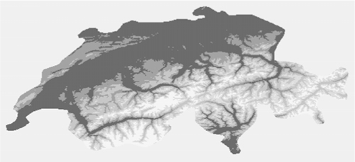
To see how color tables work, let’s create one for an elevation dataset that has been classified into ranges. This file has been created for you and is in the book data’s Switzerland folder. It’s called dem_class.tif, and the elevation values have been classified into five different ranges, so the pixel values range from 0 to 5, with 0 being set to NoData. If you look at this file in something like Windows Photo Viewer, you’ll only see a black rectangle, because that’s how it interprets such small pixel values. If you open it up in QGIS or another GIS package, it’s likely that the software will automatically stretch the data for you so you’ll see something like figure 10.7.
Figure 10.7. Digital elevation model for Switzerland that has been classified into five elevation ranges and then stretched so that the small pixel values appear different from one another
If you add a color map to this image, then it will draw correctly without being stretched, and you can specify the colors that are used for each elevation range. Let’s try it.
Listing 10.3. Add a color map to a raster

The first part of this listing doesn’t have anything to do with the color table; it’s making a copy of the image so that the original doesn’t get modified. The interesting part is when you create an empty color table called colors and then add colors to it. The first parameter to SetColorEntry is the pixel value that you want to set the color for, and the second parameter is a tuple or list containing the red, green, and blue values for the color. You set colors for pixel values between 1 and 5, inclusive. Because this is a byte dataset, there are 255 possible pixel values and the color table contains zeros (black) for the values that you didn’t change. Finally, you add the color map to the band and tell the band that it’s using a color map by setting the color interpretation to paletted, although that second step isn’t necessary because GDAL figures it out. Now your image looks like figure 10.8, although software that doesn’t understand the NoData setting will draw a black background.
Figure 10.8. Digital elevation model for Switzerland that has been classified into five elevation ranges and then had a color map applied. If you look at the color version online, it will look much different from the automatic symbology shown in figure 10.7.

You can also edit existing color tables. Say you want to change the color map you created so that the highest elevation range displays as something closer to white. Grab the color table from the band and change the entry you’re interested in, which is the pixel value 5 in this case:

Remember to open the dataset for writing. If you don’t, your changes won’t take effect and you won’t get an error message, either. You also need to add the color map back to the band because the one you’re editing is no longer linked to the band.
10.3.1. Transparency
Have you ever seen colors referred to as RGBA instead of plain RGB? The A stands for a fourth value called alpha, which is used to specify opacity. The higher the alpha value, the more opaque the color. You can add an alpha band to your image and then certain software packages, such as QGIS, will use it. Others, like ArcMap, ignore the alpha band when using color tables. If you want to go this route with color tables, you need to create your dataset with two bands, where the first one is your pixel values as before, and the second one holds alpha values. You also need to specify that this second band is an alpha band at creation time, like this:
ds = driver.Create('dem_class4.tif', original_ds.RasterXSize,
    original_ds.RasterYSize, 2, gdal.GDT_Byte, ['ALPHA=YES'])
Then add values between 0 and 255 to your alpha band, where 0 means fully transparent and 255 is fully opaque. We’ll talk about NumPy in the next chapter, but this is how you’d use NumPy to find all pixels in the first band that are equal to 5 and set them approximately 25% transparent:
import numpy as np
data = band1.ReadAsArray()
data = np.where(data == 5, 65, 255)
band2.WriteArray(data)
band2.SetRasterColorInterpretation(gdal.GCI_AlphaBand)
Here you use the NumPy where function to create a new array based on the values of the original data array from band 1. It’s like an if-else statement, where the condition is whether or not the pixel value is equal to 5. If it is, then the corresponding cell in the output array gets a value of 65, which is roughly a quarter of 255. If the original pixel has a value other than 0, then the output gets a value of 255, which is no transparency. Write that new array to the second band, and make sure you set the color interpretation for that band to alpha.
If you wanted to create an image with transparency that more software will understand, then you could create a four-band image and forego the color map. In this case, you’d put the red value in the first band, green in the second, blue in the third, and the alpha value in the fourth band. The disadvantage to this is that your dataset would be at least twice as large because it would have twice as many bands. It would probably have even another band to hold your original pixel values instead of only color information. Otherwise, you’d lose your information about pixel classifications, such as landcover types.
10.4. Histograms
Sometimes you need a frequency histogram for pixel values. One example of this would be calculating the area of each vegetation type in a vegetation classification. If you know how many pixels are classified as pinyon-juniper, for instance, then you can multiply that number by the area of a pixel (which is pixel width times pixel height) to get the total acreage of pinyon-juniper.
The easiest way to get a histogram is to use the GetHistogram function on a band. You can specify exactly what bins you want to use, but the default is to use 256 of them. The first one includes values between -0.5 and 0.5, the second bin goes from 0.5 to 1.5, and so on. So if you have byte data, this histogram will have one bin per possible pixel value (0, 1, 2, and so on). If no histogram data already exist for the raster, then this function computes an approximate one by default, but you can request an exact one. The function looks like this:
GetHistogram([min], [max], [buckets], [include_out_of_range], [approx_ok],
            [callback], [callback_data])
- min is the minimum pixel value to include in the histogram. The default value is 0.5.
- max is the maximum pixel value to include in the histogram. The default value is 255.5.
- buckets is the number of bins you want. The size of the bins is determined by taking the difference between max and min and dividing that by buckets. The default value is 256.
- include_out_of_range denotes whether or not to lump pixel values below the minimum value into the minimum bin, and the pixel values larger than the maximum into the maximum bin. The default value is False. Use True if you want to enable this behavior.
- approx_ok denotes whether or not it’s okay to use approximate numbers, either by looking at overviews or only sampling a subset of the pixels. The function will run faster this way. The default value is True. Use False if you want exact counts.
- callback is a function that’s called periodically while the histogram is being computed. This is useful for showing progress while processing large datasets. The default value is 0, which means you don’t want to use a callback function.
- callback_data is data to pass to the callback function if you’re using one. The default value is None.
This code snippet shows the difference between approximate and exact values, using the classified elevation raster that we looked at earlier:
os.chdir(r'D:osgeopy-dataSwitzerland')
ds = gdal.Open('dem_class2.tif')
band = ds.GetRasterBand(1)
approximate_hist = band.GetHistogram()
exact_hist = band.GetHistogram(approx_ok=False)
print('Approximate:', approximate_hist[:7], sum(approximate_hist))
print('Exact:', exact_hist[:7], sum(exact_hist))
The histogram consists of a list of counts, in order by bin. In this case the first count corresponds to pixel value 0, the second to pixel value 1, and so on. Here you only print the first seven entries, because the remaining 249 of them are all 0 for this dataset. The results are shown here and in figure 10.9:
Approximate: [0, 6564, 3441, 3531, 2321, 802, 0] 16659
Exact: [0, 27213, 12986, 13642, 10632, 5414, 0] 69887
Figure 10.9. The approximate and exact histograms generated from the classified elevation raster

Notice that the numbers, including the sum, for the approximate histogram are much smaller than those for the exact. Therefore, the approximate numbers are not the way to go if you need to tabulate area, but they’d probably work well if you want relative frequencies. Also notice that no counts exist for a pixel value of 0. That’s because 0 is set to NoData, so it gets ignored.
GDAL stores these histograms in an XML file alongside the raster. If you ran this code, there should now be a file called dem_class2.tif.aux.xml in your Switzerland folder. If you open it and take a look, you’ll see both sets of histogram data. As long as you don’t delete that file, those specific histograms won’t need to be computed again because GDAL can read the information from the XML file.
You can also set a certain binning scheme to be the default for an image. For example, say you want to lump pixel values 1 and 2 together, 3 and 4 together, and leave 5 alone. You can do that like this:
hist = band.GetHistogram(0.5, 6.5, 3, approx_ok=False)
band.SetDefaultHistogram(1, 6, hist)
In this example, you create a histogram with three bins that include pixel values 1 through 6. Why go up to 6 instead of 5, when the actual data values only go up to 5? The bins are created of equal size, so if there were three bins between 1 and 5, then the breaks would be in the wrong places. The breaks for the example would be at 2.5 and 4.5, but they would be at 2.2 and 3.8 if you used a range of 5 instead of 6. In that case, the pixels with values 4 and 5 would be lumped together and 3 would be alone, which isn’t the desired outcome (figure 10.10).
Figure 10.10. The results of creating three bins between 0.5 and 6.5 (A) and 0.5 and 5.5 (B). In case A, values 1 and 2 share a bin, 3 and 4 share a bin, and 5 has a bin to itself (there are no pixels with a value of 6). In case B, however, value 3 is the one that doesn’t share a bin.

Once you compute the histogram, you set it as the default. The SetDefault-Histogram function wants a minimum pixel value, maximum value, and then the list of counts. Once you’ve set a default, you can use GetDefaultHistogram to get that particular one. While GetHistogram returns a list of counts, GetDefaultHistogram returns a tuple containing the minimum pixel value, maximum pixel value, number of bins, and a list of counts:
min_val, max_val, n, hist = band.GetDefaultHistogram()
print(hist)
[40199, 24274, 5414]
When you call GetHistogram, you provide the min and max values and the number of bins to use, so that function doesn’t need to return that information because you already know it. These values are returned when you call GetDefaultHistogram because you might not know what values were used to create the default histogram.
10.5. Attribute tables
Integer raster datasets can have attribute tables, although in my experience they don’t have nearly as many fields as vector attribute tables. Instead of a record in the table corresponding to an individual feature, each record of a raster attribute table corresponds to a particular pixel value. For example, all pixels with a value of 56 will share the same record in the attribute table, because each pixel doesn’t represent an individual feature, but multiple pixels with the same value should represent the same thing, whether it’s a certain color, an elevation, a land use classification, or something else.
An attribute table doesn’t even make sense for many rasters. I can’t think of an attribute I would want to attach to various pixel values in an aerial photo, for example. In fact, raster attribute tables make the most sense for categorical data such as landcover or soil type, when you’d want attributes containing information about each category.
Let’s create an attribute table for the classified elevation raster we’ve been working with. Table 10.2 shows the elevation classes used to create the dataset, which would be useful information to store.
Table 10.2. Pixel values and the corresponding elevation ranges for the classified elevation raster
|
Pixel value |
Elevation range (meters) |
|---|---|
| 1 | 0 – 800 |
| 2 | 800 – 1300 |
| 3 | 1300 – 2000 |
| 4 | 2000 – 2600 |
| 5 | 2600+ |
We’ll use the code in the following listing to add the information from table 10.2 along with the histogram counts to the raster’s attribute table.
Listing 10.4. Add an attribute table to a raster

When you create a new raster attribute table, you need to define the columns it will have. You provide three pieces of information when you add a column. The first is the name of the column. The second is the data type, which can be one of GFT_Integer, GFT_Real, or GFT_String. The last thing is the purpose of the column using one of the GFU constants from appendix E. (Appendixes C through E are available online on the Manning Publications website at https://www.manning.com/books/geoprocessing-with-python.) The desktop software I use either doesn’t support raster attribute tables at all (QGIS) or doesn’t see most of them as anything special (ArcGIS), but there’s probably software out there that does. Therefore, the only types I’m usually interested in are the ones used here. You used GFU_Name for the column containing the pixel values, GFU_PixelCount for the histogram counts, and GFU_Generic for the description. You also told it that there will be six rows.
The next step is to add the data. You know the pixel values range from 0 to 5, so you use the range function to get a list containing those numbers and then add that list to the first column, which is pixel values. The first parameter to WriteArray is the data to put in the column, and the second parameter is the index of the column that you want to add the data to. Because you already specified that there were six rows, you’d have gotten an error about too many values if you’d provided a list with more than six items. You don’t have to write all rows at once, though. If you’d only provided four values, it would have filled the first four rows of the column. An optional third parameter tells it which row to begin writing data on, so you could then add the remaining data by passing a 4 as the last parameter so that it would start writing on the correct row.
You use this same method to add the histogram counts to the second column, except this time the list of values comes from the GetHistogram function. Remember that the 0 values are ignored when computing histograms, but you might want the number of zeros in the attribute table. One way to get a histogram that includes those values is to set NoData to a bogus value and then calculate a histogram that hasn’t been calculated before. It needs to be a new histogram because if that particular one has already been calculated, then GDAL will pull the information out of the XML file you saw earlier, and the zeros still won’t be counted. That’s why you set NoData to -1 before creating the attribute table, and then use a set of parameters that you haven’t yet used to retrieve a histogram. Conveniently, you tell it that you want six bins, which is exactly how many rows the table has.
Then you set the elevation ranges. You could create a list holding those descriptions, but instead you add each one individually by specifying the row, then the column, and then the value to put in the table. You don’t bother adding a description for the first row with index 0, because there’s not much to say about NoData.
Once you add all of your data to the table, you add it to the band with SetDefaultRAT, and then make sure to restore the NoData value to your band. Figure 10.11 shows a screenshot of this raster attribute table in ArcGIS. Unfortunately, you can’t view the results with QGIS.
Figure 10.11. Raster attribute table for the classified elevation raster

10.6. Virtual raster format
The GDAL virtual format (VRT) isn’t another property you can add to a raster, like an attribute or color table, but it’s a useful format that allows you to define a dataset using an XML file. Virtual raster datasets use other datasets to store the data, but the XML describes how to pull the data out of those other files. A VRT can be used to subset the data, modify properties such as the projection, or even combine multiple datasets into one. In these cases, the original datasets aren’t changed, but the modifications are made to the data in memory when it’s read by the software.
For example, say you had a raster dataset that covered a large spatial area, but you needed to run different analyses on various spatial subsets of the original raster. You could clip out the areas you need, or you could define a VRT for each of these subsets and not have to create the subsetted rasters on disk. For even more information on VRTs than you will see here, check out http://www.gdal.org/gdal_vrttut.html.
Before we look at manipulating data with a VRT, let’s look at an extremely simple example (called simple_example.vrt in the Landsat/Washington data folder). This XML defines a VRT dataset with one band, and that band is the blue band from the natural color GeoTIFF you created in the last chapter.
Listing 10.5. XML to define a VRT dataset with one band

This XML contains general dataset information such as the numbers of rows and columns, the spatial reference system, and the geotransform. The SRS needs to be in WKT, which would have taken up a lot of space, so I opted to truncate it for the example (the third line). In real life, you’d need the entire SRS string. There’s also a VRTRasterBand element for each band in the dataset, which is only one in this case. This contains the data type, band number, rows and columns, and the information required to load the data. This is a simple case, so it only needs a filename and a band number. You want the blue band, which is the third one in nat_color.tif. The relativeToVRT attribute tells it whether or not the file path to the data is relative to the location of the VRT file itself. If you want an absolute filename, use a 0 here. In this particular case, the image file and the VRT file are in the same directory, but if you were to move the VRT file without moving the image file, the VRT would be unable to load any data.
Creating VRT datasets from Python can be a bit tricky because you need to supply part of the XML yourself. The most basic example is providing the source filename and band number. You could set up an XML template something like the following and then use it when adding bands to the VRT:
xml = '''
<SimpleSource>
  <SourceFilename>{0}</SourceFilename>
  <SourceBand>1</SourceBand>
</SimpleSource>
'''
This snippet assumes that you’ll always use the first band from the source raster. That’s because you’re going to use it to define a natural color raster without copying any data around like you did in the last chapter, and each of the input rasters only has one band anyway. Most things work the same way with a VRT as they do for other dataset types, so creating the new dataset is the same as before. Even though no data will be copied, you still need to make sure that you create the dataset with the same dimensions as the originals:
os.chdir(r'D:osgeopy-dataLandsatWashington')
tmp_ds = gdal.Open('p047r027_7t20000730_z10_nn30.tif')
driver = gdal.GetDriverByName('vrt')
ds = driver.Create('nat_color.vrt', tmp_ds.RasterXSize,
    tmp_ds.RasterYSize, 3)
ds.SetProjection(tmp_ds.GetProjection())
ds.SetGeoTransform(tmp_ds.GetGeoTransform())
Now you can go about adding the links to the three input rasters. For each one, you need to create a dictionary with one entry, where the key is 'source_0' and the value is the XML string containing the filename. Then you add that dictionary as metadata for the band in the 'vrt_sources' domain. Repeat this process for all three bands.
metadata = {'source_0': xml.format('p047r027_7t20000730_z10_nn30.tif')}
ds.GetRasterBand(1).SetMetadata(metadata, 'vrt_sources')

metadata = {'source_0': xml.format('p047r027_7t20000730_z10_nn20.tif')}
ds.GetRasterBand(2).SetMetadata(metadata, 'vrt_sources')

metadata = {'source_0': xml.format('p047r027_7t20000730_z10_nn10.tif')}
ds.GetRasterBand(3).SetMetadata(metadata, 'vrt_sources')
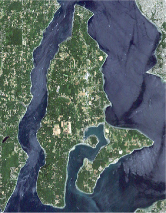
Now you can use QGIS to open the VRT dataset, and you’ll see a three-band image such as that shown in figure 10.12. Unlike the GeoTIFF you created before, this won’t open up in regular image-processing software, however.
Figure 10.12. Stacked VRT created from three single-band images. It doesn’t look like much when printed in black and white, but you can view the color version online, which will look like natural color (the way our eyes would see it).

10.6.1. Subsetting
I mentioned earlier that you can use VRTs to subset images without creating another subsetted image. The process of creating the empty dataset is similar to what you did in the previous chapter when subsetting. You still need to figure out the numbers of rows and columns and the new geotransform, and then use that information to create the new dataset. That’s what the first part of the following listing does, except that it uses a VRT driver. Things change after you create the dataset, however, because in this example you need to create the appropriate XML for each raster band and insert it into the VRT. The process is explained after the code listing.
Listing 10.6. Subset a raster using a VRT


As mentioned right before the code listing, you have to create XML to subset your raster with a VRT. This XML is slightly more complicated than the XML you used a minute ago, because it also includes elements for the source and destination extents. The numbers of rows and columns are the same size for both the source and destination and are the numbers you calculate. The offsets for the source are the offsets you compute to correspond with the upper-left corner of the area of interest, and the offsets for the destination are both 0 because you fill the entire output image:
<SrcRect xOff="{xoff}" yOff="{yoff}" xSize="{cols}" ySize="{rows}" />
<DstRect xOff="0" yOff="0" xSize="{cols}" ySize="{rows}" />
This time you use named placeholders in the XML to make it easier to see what goes where. To format this string, you need a dictionary with the same keys as placeholders. You can create this dictionary once and then change the band number (because you’re using a different band from the three-band input image each time) when you add a new band to the VRT:
data['band'] = 2

meta = {'source_0': xml.format(**data)}
ds.GetRasterBand(2).SetMetadata(meta, 'vrt_sources')
If all went well, the VRT will look like figure 10.13 if you open it in QGIS, and it will overlay perfectly on the original image.
Figure 10.13. Subsetted VRT
10.6.2. Creating troublesome formats
Not all raster formats allow you to create and manipulate multiple-band images. For example, if you’d tried to create a natural color JPEG instead of a TIFF in the previous chapter, you would have run into problems because the JPEG driver doesn’t allow you to create a multiband image and then add data to the bands. That’s a real problem if you want JPEG output! Fortunately, VRTs can come to your rescue. All you need to do is create a VRT that defines the output you want, and then use the JPEG (or whatever format) driver’s CreateCopy function. For example, to create a JPEG of Vashon Island, open up the VRT you created in the last section and then copy it to a JPEG:
ds = gdal.Open('vashon.vrt')
gdal.GetDriverByName('jpeg').CreateCopy('vashon.jpg', ds)
If you’d rather create an intermediate TIFF instead of a VRT, go right ahead, and then copy the TIFF to a JPEG. The advantage to using a VRT is that you’re not creating possibly large intermediate files on disk.
10.6.3. Reprojecting images
Remember talking about reprojecting vector data in chapter 8? Raster data can also be reprojected, but it’s more complicated than with vector data. With vectors, you need the new coordinates for each vertex and you’re good to go, but with rasters you need to deal with the fact that cells get bent and moved around, and a one-to-one mapping from old cell locations to new cell locations doesn’t exist (see figure 10.14). The easiest way to determine the pixel value for a new cell is use the value from the input cell that gets mapped closest to the output cell. This is called nearest-neighbor and is the fastest method, the one you’ll usually want for categorical data. All others, except mode, will change your categories, which you definitely don’t want for categorical data. Continuous data rasters usually won’t look good if you use nearest-neighbor, however. For those, I generally use bilinear interpolation or cubic convolution, which use an average of surrounding pixels. Several other methods are available, however, that might be more appropriate for your particular data.
Figure 10.14. Example of how pixels get moved around when the raster is projected. The triangles and circles are pixel center points for two different rasters. The triangles were created from a reprojected version of the raster that the circles came from. Notice that the dimensions are even different.

I think that the easiest way to reproject a raster, other than using the gdalwarp utility that comes with GDAL, is to use a VRT. There’s a handy function that creates a reprojected VRT dataset for you when you provide the spatial reference information. It looks like this:
AutoCreateWarpedVRT(src_ds, [src_wkt], [dst_wkt], [eResampleAlg],
[maxerror])
- src_ds is the dataset you want to reproject.
- src_wkt is the WKT representation of the source spatial reference system. The default is None, in which case it will use the SRS information from the source raster. If this raster doesn’t have SRS information, then you need to provide it here. You can also provide it here if using None makes you nervous.
- dst_wkt is the WKT representation of the desired spatial reference system. The default is None, in which case no reprojection will occur.
- eRasampleAlg is one of the resampling methods from table 10.3. The default is GRA_NearestNeighbour.
Table 10.3. Resample methods
Constant
Description
GRA_NearestNeighbour Closest pixel GRA_Bilinear Weighted distance average of 4 pixels GRA_Cubic Average of 16 pixels GRA_CubicSpline Cubic B-spline of 16 pixels GRA_Lanczos Lanczos windowed sinc with 36 pixels GRA_Average Average GRA_Mode Most common value - maxerror is the maximum amount of error, in pixels, that you want to allow. The default is 0, for an exact calculation.
The AutoCreateWarpedVRT function doesn’t create a VRT file on disk, but returns a dataset object that you can then save to another format using CreateCopy. The following example takes the natural color Landsat image that uses a UTM spatial reference, creates a warped VRT with a destination SRS of unprojected WGS84, and copies the VRT to a GeoTIFF:
srs = osr.SpatialReference()
srs.SetWellKnownGeogCS('WGS84')
os.chdir(r'D:osgeopy-dataLandsatWashington')
old_ds = gdal.Open('nat_color.tif')
vrt_ds = gdal.AutoCreateWarpedVRT(old_ds, None, srs.ExportToWkt(),
    gdal.GRA_Bilinear)
gdal.GetDriverByName('gtiff').CreateCopy('nat_color_wgs84.tif', vrt_ds)
The output from this looks like figure 10.15.
Figure 10.15. The original Landsat image that uses a UTM spatial reference, and the new one that uses unprojected lat/lon coordinates

10.7. Callback functions
Often you want an indication of how long your process is going to take or how far along it is. If I’m batch processing multiple files, and each one takes a long time, I’ll sometimes have my code print out a message telling me which file it’s currently working on. That’s not a useful technique if I want to see the progress of a GDAL function, such as computing statistics or warping an image, because that bit of processing is out of my hands once I call the function. Fortunately, the GDAL developers thought of this, and many functions take callback functions as arguments (in fact, you saw this in the signature for Get-Histogram). A callback function is one that gets passed to another function and is then called from the function it was passed to (figure 10.16).
Figure 10.16. Callbacks are functions that get passed as parameters to a second function, where they’re later called.

In the case of GDAL, the callback functions are designed to show progress, so they get called often as the process runs. A predefined function is even available for you to use that prints a percentage or a dot at every 2.5% of progress. By the time the process has finished, the output from this function looks like this:
0...10...20...30...40...50...60...70...80...90...100 - done.
To take advantage of this, just pass gdal.TermProgress_nocb to any function that takes a callback function as a parameter. This example would cause progress information to be printed while calculating statistics:
band.ComputeStatistics(False, gdal.TermProgress_nocb)
Tip
Several of the methods on OGR layers, such as Intersection and Union, also accept a callback parameter. To use it, import GDAL and pass gdal.TermProgress_nocb as you do with GDAL functions. You could also use callbacks to track the progress of your vector-processing functions using the techniques shown here.
You can also use this function to print out the progress of your own functions. Instead of passing the TermProgress_nocb function to another function, call it yourself with the appropriate percentage. For example, if I wanted to use this instead of print filenames during my batch processing, I could do something like this:
for i in range(len(list_of_files)):
    process_file(list_of_files[i])

    gdal.TermProgress_nocb(i / float(len(list_of_files)))
gdal.TermProgress_nocb(100)
This assumes that the list_of_files variable is a list of all of the files to process, and that the process_file function does something with the file. Each time I start processing a new file, I figure out how far I am based on the total number of files and pass that to TermProgress_nocb so I can get a visual indication of my progress. The progress function is also called after finishing the loop in order to tidy things up. Otherwise, if the last percentage passed wasn’t quite 100, you’d end up with output like this, where the last bit is missing:
0...10...20...30...40...50...60...70...80...90..
You might not care about that, but if other people are running your code, they might prefer to know that things finished.
Note
It’s possible that with your version of GDAL, the progress function is called TermProgress instead.
You can also write your own callback function if you’d like your progress information to look different. The function you define needs to have three different parameters. The first is the progress percentage between 0 and 1, the second is a string, and the third is whatever you want. If one of the GDAL functions invokes your callback, it will pass a string specifying what it’s doing as the second parameter. You provide the third parameter when you pass in the callback function. The best way to explain how this works is by example, so the following listing is an example that allows the user to specify how often to print a progress indicator dot by passing in another number between 0 and 1 as the progressArg parameter. The message string is also printed out once at the beginning.
Listing 10.7. Use a callback function

There’s a trick here that you may not have seen before. Normally when you declare a variable inside a function, it disappears when the function finishes, right? Here you attach the variable to the function as an attribute, so it sticks around and can be used the next time the function is called. The Python hasattr function checks to see if an object has an attribute with a given name, and you check to see if the my_progress function has an attribute called last_progress. If there isn’t one, then you assume that this is the first time the function has been called and print the message parameter and create the last_progress attribute. The next time the function is called, that attribute will exist, so the message won’t be printed. You’ll also use that attribute to keep track of how many dots have been printed so far.
Next you check to see if the process is done. If so, then you print done and delete the last_progress attribute. If you don’t delete the attribute, then you can’t use this function again in the same script because it will always think that it’s done and won’t do anything.
If the process isn’t finished, which is the case most of the time, you use divmod (which returns a quotient and a remainder as a tuple) to figure out how many dots should be printed. Because multiple dots might need to be printed if the process runs quickly, you keep printing and incrementing last_progress until it equals the required number of dots.
This function uses sys.stdout.write instead of print because print works slightly differently in Python 2 and 3, and so you need to call it in different ways to get the dot to print without a newline after it. Using write solves the problem because it doesn’t print a newline unless you request it. You do need to call flush to make sure that the dot shows up immediately, however. The progress function isn’t of much use if the dots aren’t printed until the processing is finished.
Now that you have your progress function, how do you use it? Exactly the same way that you used TermProgress_nocb, except that you need to include an additional parameter specifying how often you want the indicators printed (the default value of 0.02 is only honored if you call the function yourself, not if it’s called by something else). Here’s an example:
band.ComputeStatistics(False, my_progress, 0.05)
Compute Statistics...................done
This is a simple example, but the same concepts apply if you want to do something more complicated. For example, if you had an exceptionally long-running process and wanted to be notified by email at certain points in the process, you could do that.
10.8. Exceptions and error handlers
As with OGR, you can have GDAL throw an exception when it runs into a problem. To do this, simply call UseExceptions, and you can turn exceptions off by calling Dont-UseExceptions. Normally, you need to make sure that operations that might have failed did work, such as opening a file. If you don’t check and the file wasn’t opened, then your script will crash when it tries to use the dataset. This might be fine, depending on what you’re doing, but it might not be. Take this simple example of batch-computing statistics:
file_list = ['dem_class.tif', 'dem_class2.tiff', 'dem_class3.tif']
for fn in file_list:
    ds = gdal.Open(fn)
    ds.GetRasterBand(1).ComputeStatistics(False)
This is great, except for the extra “f” at the end of the second filename. The script will spit out the following error and crash when it tries to get the band, and the last file will never be looked at:
ERROR 4: `dem_class2.tiff' does not exist in the file system,
and is not recognised as a supported dataset name.

Traceback (most recent call last):
  File "D: errors.py", line 28, in <module>
    ds.GetRasterBand(1).ComputeStatistics(False)
AttributeError: 'NoneType' object has no attribute 'GetRasterBand'
You have a few ways you can solve this problem. You might have your code check that the dataset was successfully opened, and if not, print a message so that the user knows that the file was skipped. This way nothing will crash and statistics will be computed for the last file:
for fn in file_list:
    ds = gdal.Open(fn)
    if ds is None:
        print('Could not compute stats for ' + fn)
    else:
        ds.GetRasterBand(1).ComputeStatistics(False)
A cleaner way to handle errors would be to use a try/except block. If multiple possible points of failure exist, you don’t have to check that each one succeeded. Instead, wrap the whole thing in one try block and handle all errors in the except clause:
gdal.UseExceptions()
for fn in file_list:
    try:
        ds = gdal.Open(fn)
        ds.GetRasterBand(1).ComputeStatistics(False)
    except:
        print('Could not compute stats for ' + fn)
        print(gdal.GetLastErrorMsg())
Although the error was encountered in this case, the error message would not print automatically. If you need it, you can get access to the error message using the GetLastErrorMsg function. After the except clause is processed, the loop continues with the next filename in the list.
GDAL also has the concept of error handlers that get called whenever a GDAL function runs into an error. The default error handler prints out error messages like the one you saw a second ago. If you don’t want these messages printed for some reason, you can shut them up with the built-in quiet error handler. To do this, enable the handler before running the code that you’d like to be quiet. The PushErrorHandler function will make a handler the active one until you call PopErrorHandler, which will restore the original handler:
gdal.PushErrorHandler('CPLQuietErrorHandler')
# do stuff
gdal.PopErrorHandler()
You can also use SetErrorHandler to enable a handler, but then it’s in effect until you pass a different handler to SetErrorHandler:
gdal.SetErrorHandler('CPLQuietErrorHandler')
# do stuff
gdal.SetErrorHandler('CPLDefaultErrorHandler')
Error handlers aren’t limited to the GDAL functions, though. You can call them yourself if you’d like. Say you have a function that takes two datasets, but they need to share a spatial reference system for your logic to work. You can call whatever error handler happens to be in effect by using the Error function, which takes three parameters. The first is an error class and the second is an error number, both from table 10.4. The third argument is the error message.
Table 10.4. Possible error classes and numbers
|
Error classes |
Error numbers (types, if you prefer) |
|---|---|
| CE_None | CPLE_None |
| CE_Debug | CPLE_AppDefined |
| CE_Warning | CPLE_OutOfMemory |
| CE_Failure | CPLE_FileIO |
| CE_Fatal | CPLE_OpenFailed |
| CPLE_IllegalArg | |
| CPLE_NotSupported | |
| CPLE_AssertionFailed | |
| CPLE_NoWriteAccess | |
| CPLE_UserInterrupt |
def do_something(ds1, ds2):
    if ds1.GetProjection() != ds2.GetProjection():
        gdal.Error(gdal.CE_Failure, gdal.CPLE_AppDefined,
            'Datasets must have the same SRS')
        return False
    # now do your stuff
You might be wondering why you would do this instead of print your error message and return from the function. You certainly could do that, but this gives you more flexibility in the future. If this function is part of a module you’re reusing in different situations, you might want to handle errors in different ways, depending on your application. This gives you that ability, because all you have to do is change your error handler instead of finding and changing all of your print statements (which you might have to change back for another application). This also makes your function treat errors the same way that GDAL does. If UseExceptions is in effect, then instead of printing the error message, the call to Error will raise an exception that can be caught in a try/except block.
You can write your own error handlers, too. You might do this so you could log error messages to a file or database, or I suppose you could also try to solve the error somehow. If you do choose to write your own function, it needs to accept the same three arguments that get passed to the Error function. Here’s a simple example of a handler that logs the error class, reason, and message using the Python logging module:
def log_error_handler(err_class, err_no, msg):
    logging.error('{} - {}: {}'.format(
        pb.get_gdal_constant_name('CE', err_class),
        pb.get_gdal_constant_name('CPLE', err_no),
        msg))
The ospybook module contains a function that helps you get the human-readable forms of the GDAL constants. Pass it the case-sensitive prefix corresponding to the type of GDAL constant you want to look up and the numeric value to find. The function returns the name of the constant as a string.
>>> import ospybook as pb
>>> print(pb.get_gdal_constant_name('GDT', 5))
GDT_Int32
You could use a function like this to easily send your error messages to different places. If you wanted to see the messages on the screen, all you’d have to do is import the logging module and set your error handler:
import logging
gdal.PushErrorHandler(log_error_handler)
To send the messages to a file instead, you need to add the step of configuring the logger, like this:
import logging
logging.basicConfig(filename='d:/temp/log.txt')
Now if you called your do_something function on two datasets with different spatial references, a line like this would get added to log.txt:
ERROR:root:CE_Failure - CPLE_AppDefined: Datasets must have the same SRS
Normally, when you turn on exceptions by calling UseExceptions, the error handlers are turned off and an exception is raised when an error is encountered. This is why the error messages don’t automatically print when exceptions are enabled. If you wanted your error message logged using your new log_error_handler function, but you also wanted to use exceptions, you could enable the error handler after enabling exceptions, and then you should get both behaviors.
10.9. Summary
- Use known locations, called ground control points, if you don’t have geotransform information for a raster dataset. You can create a geotransform from the GCPs.
- Add a raster attribute table to your thematic datasets so that you know what each pixel value means.
- Add a color table to a thematic dataset if you want it to draw with the same colors all of the time.
- You can manipulate data with virtual raster files without ever creating new files on disk.
- The easiest way to reproject a raster is to use a VRT and then copy it to the desired format.
- It’s a good idea to use callback functions to provide progress information for long-running processes.