Chapter 9: Use of the VARMAX Procedure to Model Multivariate Series

Introduction

Use of PROC VARMAX to Model Multivariate Time Series

Dickey-Fuller Tests for Differenced Series

Selection of Model Orders

Fit of a Fourth-Order Autoregressive Model

Estimation for the Parameters

Restriction of Insignificant Model Parameters

Residual Autocorrelation in a VARMA(2,0) Model

Cross-Correlation Significance

Portmanteau Tests

Distribution of the Residuals in a VARMA(2,0) Model

Identification of Outliers

Use of a VARMA Model for Milk Production and the Number of Cows

Analysis of the Standardized Series

Correlation Matrix of the Error Terms

The Model Fit

Properties of the Fitted Model

Conclusion

Introduction

In this chapter, PROC VARMAX is introduced for estimating the parameters of multivariate time series models. The VARMAX procedure is relatively new. It was introduced in SAS 8.1 and expanded in subsequent releases of SAS and the releases of Analytical Updates. The procedure name VARMAX is an initialism for Vector AutoRegressive Moving Average with EXogenous variables. It includes features for multidimensional time series analysis using exogenous variables (as indicated by the name of the procedure):

•   Cointegration

•   Generalized autoregressive conditional heteroscedasticity (GARCH) models for volatility

•   Bayesian methods

Moreover, many popular tests within econometrics are included. Among these are Dickey-Fuller tests for stationarity, Granger causality tests, Jarque-Bera tests for normality, and Johansen rank tests. The procedure is rather advanced, and its use requires a little more programming than simpler procedures such as PROC REG.

As a first example of how the procedure works for multivariate time series, two historical time series for the Danish economy are considered in this chapter. The example of the number of cows and milk production from the previous chapters is continued in the last part of this chapter.

Use of PROC VARMAX to Model Multivariate Time Series

Here the WagePrice data set introduced in Chapter 7 is applied. The variables are as follows, where P denotes the series of a Danish price index and W similarly denotes the series of a Danish wage index for the years 1818 to 1981:

LP = log(P)

LW = log(W)

The basic application of PROC VARMAX for simultaneously modeling the two series, the log-transformed wage and price indices, and using differences, is simple, as seen in Program 9.1. The differences are explicitly stated for both series by the DIF option.

Program 9.1: A Simple Application of PROC VARMAX for a Two-Dimensional Series

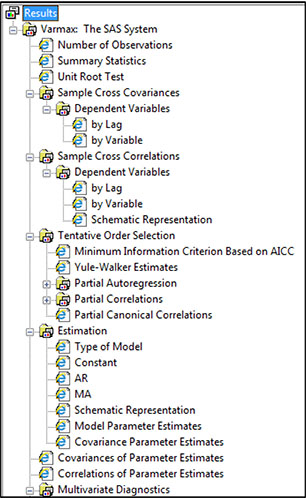
This output contains the same elements as for a one-dimensional series, but it is, of course, longer because two series are analyzed. The RESULTS window gives a summary of all the generated output. Output 9.1, which is printed over many pages, gives this overview of all output elements as all subfolders are unfolded in the display. The output consists of three main parts: basic statistical properties of the series, estimation of a particular model, and checks of the fitted model. Because the options PRINTALL and PLOTS=ALL are used, many more features of the model are presented, which leads to a lengthy output. Some of the output elements, which help understanding the estimated model, are discussed in Chaper10.

Output 9.1: Summary of All Generated Output from Program 9.1

Dickey-Fuller Tests for Differenced Series

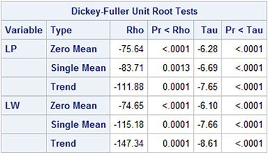
The series of first differences pass the Dickey-Fuller testing because the test statistics clearly reject the hypothesis of a further differencing (Output 9.2). Note that the Dickey-Fuller test in PROC VARMAX includes no augmented lags (see Chapter 5). The reported statistics in Output 9.2 are exactly the same as were reported for the differences of the univariate series in Chapter 7, Output 7.2.

Output 9.2: Dickey-Fuller Test for Two Time Series

Because no model orders are specified in Program 9.1, a model is found by a model order choosing device, which optimizes a criterion of fit. The default criterion of fit is the corrected Akaike Information Criterion (AICc; see Chapters 6 and 8).

Selection of Model Orders

For this data, model selection using the corrected Akaike Information Criterion (AICc) ends up with a model having p = 4 and q = 1. The model selection is reported in a table of criteria values for all possible models p ≤ 5 and q ≤ 5 (Output 9.3). The optimal value −11.83727 is, however, not remarkably smaller than the other values. Moreover, it turns out from the estimated parameters that all entries of the estimated moving average coefficient are insignificant.

Output 9.3: Corrected Akaike Information Criterion for Potential VARMA Models

In Program 9.2 the criterion for selection is changed to the Schwartz Bayesian Criterion (SBC) as opposed to the default corrected Akaike Criterion (AICc), by the option MINIC, which is an abbreviation for minimum information criterion. Moreover, only autoregressive models are included in the model selection by the option Q = 0 to the MINIC option in the MODEL statement.

Program 9.2: Specifying the Model Selection Procedure

In this setup, a first-order autoregressive model, p = 1, is best (Output 9.4) because the criterion value −11.38 is the smallest value in the table. The fit of this model is not satisfactory, however, because the residual correlations are significant for many lags, meaning that the residuals are dependent. This rejection of the model is seen by all fit diagnostics for the model. Applications of for these fit diagnostics are presented in later sections. The conclusion of this section could be that this automatic model selection leads to models that can be applied in practice, but further care is required if the end goal is a genuine analysis with a proper statistical model.

Output 9.4: SBC for Autoregressive Models of Orders up to 5

Fit of a Fourth-Order Autoregressive Model

In Program 9.3, an autoregressive model of order 4 is selected by the option P=4. Its parameters are estimated by the method of maximum likelihood because of the option METHOD=ML. This method is the default for most models, but for consistency it is included in applications of PROC VARMAX in this book.

Program 9.3: Specifying the Model as VARMA(4,0)

Estimation for the Parameters

The schematic representation of the parameters (Output 9.5) tells by a quick glance the significance and the signs of the estimated parameters. Insignificant entries in the autoregressive matrices are indicated by a dot. The symbols + and − represent parameters that are significant at the .05 level. All but one of the parameters for lags 3 and 4 are seen to be insignificant (Output 9.5). So it is relevant to test whether the order of the model could be reduced, or, alternatively, whether some particular entries of the matrices of autoregressive parameters could be set to 0. This consideration is important because the number of autoregressive parameters of a fourth-order model for a two-dimensional vector time series is large—in fact 16.

Output 9.5: Estimated Parameters from Program 9.3

You can test for the hypothesis that the order of the autoregressive model can be reduced from 4 to 2 by testing that all 8 entries in the matrix of autoregressive coefficients for both lag 3 and lag 4 are 0. In PROC VARMAX, such testing is performed by a test statement (Program 9.4), where all particular coefficients set to 0 are specified.

Program 9.4: Restricting Parameters to 0 in a VARMA(4,0) Model

The test leads to a rejection as seen in Output 9.6. The degrees of freedom for the test are 8 because a hypothesis specifying the values of 8 parameters is tested.

Output 9.6: Test Result for Reduction of the Order from 4 to 2

It is clear from Output 9.5, however, that only one element, the entry (1,1) of the matrix at lag 4, is significantly nonzero, as seen in the schematic presentation of the estimated model parameters (see Output 9.5). This is the element that gives the effect of the price series to itself with a lag of 4 years. Moreover, one entry in the autoregressive matrices at lag 2 is likely to be 0 (again see Output 9.5).

Restriction of Insignificant Model Parameters

In Program 9.5, all seemingly insignificant coefficients in the fitted VAR(4) model are restricted to 0, while only the significant coefficients from the full fourth-order autoregressive model are estimated. The hypothesis that all these parameters could be restricted to 0 is borderline accepted, p = .047. This test is performed by replacing the RESTRICT statement in Program 9.5 with a TEST statement.

Program 9.5: Restricting All Insignificant Coefficients

The resulting model is perhaps most easily understood if you look at its matrix representation (Output 9.7). Here, the four two-by-two estimated autoregressive matrices φ₁, .., φ₄ are printed on top of each other. The zeros represent all the restricted parameters, while the remaining estimates are all significant.

Output 9.7: Estimated Parameters from Program 9.5

This model is a fourth-order autoregressive model of the differenced series of the price index (the variable LP). The model is similarly a second-order autoregressive model for differenced series of the wage index (the variable LW). Moreover, changes in LP affect LW at lags 1 and 2, and LW affects LP at lags 1 and 2. So the two series interact with some time delays.

The estimated model is of the following form written as two individual equations:

ΔX_1t =  .27ΔX_1t−1 + .33ΔX_2t−1 − .26ΔX_2t−2 + .18ΔX_1t−4 + ε_1t

ΔX_2t =  .21ΔX_1t−1 + .58ΔX_2t−1 − .21ΔX_1t−2 + .38ΔX_2t−2 + ε_2t

Here, ΔX_1t denotes the differenced log-transformed price series LP, and ΔX_2t denotes the differenced log-transformed price series LW.

One of the restricted parameters seems to be clearly significant as judged by the provided tests for the individual restrictions (Output 9.8). These tests are Lagrange multiplier tests for the hypothesis that each of the restrictions is valid.

Output 9.8: Tests for the Restrictions in Program 9.5

If you follow the principle of parsimony, it is, however, natural to conclude that the model is acceptable as it is and that inclusion of more parameters is useless even if 2 restrictions at lag 3 and lag 4 are rejected by the test results in Output 9.8. The only estimated parameter for lag 4, AR_4_1_1 = 0.18, is close to zero. If this parameter is also left out of the model, the model turns into a compact, second-order model, which is more attractive because of its simplicity.

In the next section, such a second-order model is applied, and the various model fit measures provided by PROC VARMAX demonstrate the ways that the model is acceptable. But the output also shows how the model in some aspects misfits the multivariate structure of the two time series.

Residual Autocorrelation in a VARMA(2,0) Model

In this section, a second-order model is considered in spite of the conclusion in the previous section that a second-order model is in fact not accepted by testing with a fourth-order model as the alternative. For the AR(2) model, two parameters at lag 2 seem to be insignificant according to their individual t-tests. In this section, these two parameters are—for simplicity’s sake—included in the estimation. In Program 9.6, the options PRINTALL and PLOTS=ALL request a lengthy output, including statistics and graphs for a careful check of model fit.

Program 9.6: Estimating the Parameters of a VARMA(2,0) Model

Cross-Correlation Significance

The output presents autocorrelation and cross-correlation diagnostics for the white noise hypothesis for the residual series. The null hypothesis is that all (apart from lag 0) autocorrelations and cross-correlations should be 0 for the residuals of the wage and the price series. The estimated autocorrelations and cross-correlations are presented as numbers in tables, and they are displayed as graphs. Their significance is shown in various ways.

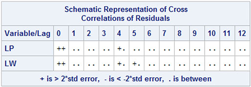
First, Output 9.9 gives a schematic presentation of all residual autocorrelations and cross-correlations. There is a clear indication that only three values are significant: namely a single autocorrelation and a cross-correlation for lag 4 and one cross-correlation for lag 5.

Output 9.9: Quick Glance at the Cross-Correlation Significance

Portmanteau Tests

The portmanteau test for the hypothesis that all autocorrelations and cross-correlations are 0 is shown in Output 9.10 for both series. The tests were introduced in Chapter 8. Only the lag 5 value is significant, but it is clear that some correlation exists around lags 4–6. The test for all lags up to lag 12 gives acceptance, p = .50.

Output 9.10: Portmanteau Tests for Residual Autocorrelation and Cross-Correlation

Figure 9.1 presents the residual autocorrelation function (ACF) for the wage series as plots of the residual autocorrelations in the upper left corner. A plot of significance of the individual autocorrelations is presented in the lower right corner of the panel. Moreover, the inverse autocorrelations (IAC) and the partial autocorrelations (PACF) are plotted in the panel that consists of 4 plots. These statistics are of importance if you must choose a specific way to improve the model, but they are not commented on further in this book. All plots indicate that the fit is accepted, because only perhaps the lag 4 value is somewhat doubtful. The similar plots for the price series point to the same conclusion.

Figure 9.1: Residual Autocorrelation for the Wage Series

Distribution of the Residuals in a VARMA(2,0) Model

Plots for the fit of the normal distribution to the prediction errors for the two series clearly point to the presence of outliers (Figures 9.2 and 9.3). The outliers disturb the normal distribution in both tails of the Q-Q plot and give long tails to the histogram.

Figure 9.2: Residual Histogram and Normality Q-Q Plot for the Wage Series

Figure 9.3: Residual Histogram and Normality Q-Q Plot for the Price Series

Identification of Outliers

From the plots of the residual series, you can see that these outliers are from the years just after the First World War for both series, as well as from 1940 for the price series and from the successive years 1856 and 1857 for the wage series (Figures 9.4 and 9.5).

Figure 9.4: Residual Plot for the Wage Series

Figure 9.5: Residual Plot for the Price Series

These outliers clearly violate the assumption of normality as tested in Output 9.11. The test for normality is the Jarque-Bera test, which is based on the empirical coefficient of skewness and kurtosis. This test indicates non-normality for both residual series, as is expected in the presence of outliers. Moreover, the outliers clustering for the post–First World War period and for the wage series, as well as for the two consecutive years 1856 and 1857, lead to the significance in the ARCH-effect testing. These tests are also provided in Output 9.11. General modeling of ARCH effects is the subject of Chapters 15 to 17. In this case, the test results are mainly due to the fact that some of the outliers are present within periods of only a few years. The Durbin-Watson test for the two residual series, also given in Output 9.11, indicates only that the first-order autocorrelations for each of the two residual series are close to 0, which is already seen in the plotted autocorrelation and the portmanteau testing.

Output 9.11: Tests for Normality and ARCH Effects for the Residual Series

Use of a VARMA Model for Milk Production and the Number of Cows

In Chapters 2 to 5, the possible interactions between the series of the number of cows and milk production in the United States were analyzed in various ways by means of traditional regression models. In this section, this example concerning the dependence between the number of cows and milk production in the United States is continued with PROC VARMAX. The number of cows series is named COWS and the milk production is denoted PRODUCTION as variables in the data set QUARTERLY_MILK.

In Chapter 7, an AR(1) model was found to fit the series of changes, from quarter to quarter, of the number of cows. Moreover, an MA(1) was estimated for the similarly differenced milk production series. Program 9.7 gives the code for estimating a VARMA(1,1) model, which is a combination of these individual models for the two univariate series.

Program 9.7: Estimating a VARMA(1,1) Model by PROC VARMAX for a Two-Dimensional Series

The model includes many parameters. Both the autoregressive coefficient matrix and the moving average matrix have four entries. The variance matrix for the error process has three parameters, and the seasonal dummies give three parameters for each series for a total of six parameters. Moreover, a constant term, an intercept, is included in the model, which gives two more parameters.

Many of the parameters are insignificant, as shown by Output 9.12. The estimated AR_1_2_1 parameter is very close to 0 with a standard deviation reported as zero in Output 9.12. This coefficient is for a right side variable, which is numerically large, while the response is numerically much smaller. This fact, of course, leads to a numerically small regression coefficient and to a standard deviation very close to 0. If this result is considered a problem, then you will need to rescale the data series. This is done in the next subsection.

Another problem is that some of the estimated moving average parameters are rather large, and their standard deviations are printed as 0. It could be due to the different scaling of the two series; but it might also be an indication that the estimation algorithm failed.

Output: 9.12: Estimated Parameters in an AR(1) Model

Analysis of the Standardized Series

In Program 9.8, the series are first standardized to mean zero and variance one. This is obtained by an application of PROC STANDARD. The standardized variables are saved in the data set named STANDARD in the WORK library.

Then an AR(1) model is estimated with all insignificant parameters from Output 9.12 restricted to zero. In fact, many parameters are restricted to zero: both the seasonal dummies for the series of number of cows and three entries out of four in the autoregressive 2 ×2 matrix. Note, for example, that the notation SD(2,3) is the parameter for the second variable to the seasonal dummy for the third quarter. Note, moreover, that the numbering of the quarters does not necessarily correspond to the number of the quarters in a year. See the discussion in Chapter 7 for details about the numbering of seasonal dummies. For this particular data set, the discussion is postponed to the” subsection “Properties of the Fitted Model.”

Program 9.8: Standardization before the Application of PROC VARMAX

The estimated parameters are presented as Output 9.13. Many parameters are insignificant, which of course is to be expected. The number of cows series when seen as a univariate series as in Chapter 7 did not show any seasonal variation. So even if seasonality could be imposed by the interaction between this nonseasonal series and the milk production series, which has highly significant components, all seasonal dummies for the number of cows series are nearly insignificant, with p = .027 as the most significant.

Output 9.13: Estimated Parameters in an AR(1) Model with Many Restrictions

Some of the VARMA parameters display the same kind of dynamics in the series, leading to individual insignificance. This is especially true when the univariate models are specified as ARMA(1,1) while they were either AR(1) or MA(1) in Chapter 7. The hypothesis that the marginal models reduce to the more simple models from Chapter 7 is tested by the TEST statement:

              TEST AR1_1_1=0,MA1_2_2=0;

The hypothesis is accepted (Output 9.14), p = .28.

Output 9.14: Testing Results for Reducing the Univariate Submodels

If these two parameters are restricted to 0 by the following RESTRICT statement, only the MA1_1_2 parameter for the interaction at lag 1 is significant:

              RESTRICT AR1_1_1=0,MA1_2_2=0;

This was also the case in the model estimated without any restrictions, Output 9.13. In Program 9.9, all 5 insignificant parameters are restricted to 0: both the 2 marginal parameters and the 3 insignificant parameters for the interaction.

Program 9.9: Estimating the Parameters in an AR(1) Model with many Restrictions and a Bound

Also, in Program 9.9, a BOUND statement is included for the MA1_1_1 parameter. This BOUND statement is included because the estimate for the MA parameter θ₁₁ otherwise equals 1.0, which is theoretically unattractive. An MA(1) parameter that is equal to ± 1 corresponds to a unit root on the moving average polynomial. An infinite order representation of the model is not possible in this situation. Output 9.15 gives the estimated parameter values.

Output 9.15: Estimated Parameters in the Final Model

The MA1_1_1 parameter is estimated to the boundary value θ₁₁ < .95. This restriction is, however, acceptable: p = .16, according to the table of tests for the individual restrictions, Output 9.16.

Output 9.16: Tests for the Restrictions and the Boundary Condition in Program 9.9

Correlation Matrix of the Error Terms

The estimated covariance matrix for the error terms is printed in Output 9.17.The correlation between the two components in the error process is as follows:

$\frac{.02955}{\sqrt{.03057\times .\text{10968}}}=.51$

Output 9.17: The Estimated Error Covariance Matrix

This correlation corresponds to the regression coefficients that were estimated for the differences in Chapter 5. The regression coefficient using the standardized number of cows (the first variable) as the response variable and the standardized milk production (the second variable) as the independent variable is as follows:

$\frac{.02955}{.03057}=.97$

This number, of course, is not equal to the value from Chapter 4 because of the standardization applied to the series in this chapter.

The Model Fit

The fit is accepted by the portmanteau tests, and the schematic representation of the cross-correlations as just a single cross-correlation is significant. This occurs at lag 10, which has no particular importance. (See Output 9.18 and Output 9.19.) This means that both the autocorrelation structure and the cross-correlation structure in the data set are fitted well by the model.

Output 9.18: Cross-Correlations of Residuals

Output 9.19: Portmanteau Tests for Model Fit

Properties of the Fitted Model

The model includes only 3 VARMA parameters. The remaining parameters are constants and seasonal dummies. The VARMA model structure is expressed as two individual equations as follows:

ΔX_1t =  ε_1t − .95ε_1t−1 + .29ε_2t−2

ΔX_2t =  .57ΔX_2t−1 + ε_2t

Here, ΔX_1t denotes the differenced standardized milk production series, and ΔX_2t denotes the differenced standardized number of cows series.

Apart from the constants and the seasonal dummies that are left out in these two formulas, the dynamic structure is simple. The numbers of cows series includes an autoregressive component. This autoregressive component indicates that if the number of cows increases from one quarter to the next quarter (a positive ΔX_2t−1)) the number of cows also tends to increase in the following quarter again by half the amount. An unexpected decrease in the milk production from one quarter to the next (a positive ε_1t−1) is totally compensated (as the MA1_1_1 parameter is nearly equal to 1) by a similar rise in the next quarter. These findings give the same conclusion as with the univariate models in Chapter 7.

The only interaction term between the two series indicates that a positive unexpected rise in the number of cows leads to a significant rise in the milk production the next quarter. This is, of course, natural in the context of the variables. The actual value of the parameter is, however, not directly interpretable because of the standardization. In the model output, Output 9.12, a first order difference is applied, and a first order autoregression is fitted. The difference operator and the autoregression then lead to two observations, which are unavailable for the estimation. Therefore, the third observation is taken as the base for the seasonal dummies. The constant value, CONST1, is negative, indicating that the milk production falls from the second to the third quarter.

The SD_1_1 parameter is positive and numerically almost equal to the CONST1. This means that the milk production is almost the same in the second and the third quarter of a year (that is, in the summertime). The remaining two seasonal dummies SD_1_2 and SD_3 are positive and numerically much larger than CONST1. This means that the milk production increases in the fourth and the first quarter of a year.

Conclusion

This chapter presented an application of PROC VARMAX to the series of Danish wages and prices for more than 100 years. In this example, the order of the model was found by the automatic order selection method available in PROC VARMAX. The model was then further simplified by testing the significance of individual parameter coefficients. The resulting model is a model with lagged dependencies in both directions that indicate that a bivariate model cannot be simplified to univariate models for the individual series.

The second example uses the quarterly series of the U.S. milk production and number of cows. The two series in the data set are measured at different scales. For numerical reasons, their interdependence is better studied by the use of standardized series. The standardized series with variance equal to 1 has regression coefficients that are more suited to the usual format with a decimal point.