4 Formula Editor

Overview

The JMP Formula Editor is a powerful tool for building formulas that calculate values for each cell in a column. The Formula Editor window operates like a calculator with buttons, displays, and an extensive list of easy-to-use features for building formulas.

JMP formulas can be built using other columns in the data table, built-in functions, and constants. Formulas can be simple expressions of numeric, character, or row state constants or can contain complex evaluations based on conditional clauses. Once created, the formula remains with the column until the formula is deleted. It is visible in both the Column Info window and in the Formula Editor itself.

A column whose values are computed using a formula is both linked and locked. It is linked to (or dependent on) all other columns that its formula refers to. Its values are automatically recomputed whenever you edit the values in these columns. It is also locked, so its data values cannot be edited, which would invalidate its formula.

This chapter describes Formula Editor features and gives a variety of examples. See the online Using JMP for a complete list of Formula Editor functions.

Chapter Contents

Overview

The Formula Editor Window

The Formula Editor and the JMP Scripting Language

A Quick Example: Standardizing Data

Making a New Formula Column

Using Popular Formula Functions

Writing Conditional Expressions

Summarizing Data with the Formula Editor

Generating Random Data

Local Variables and Table Variables

Working with Dates

Tips on Building Formulas

Examining Expression Values

Cutting, Dragging, and Pasting Formulas

Selecting Expressions

Exercises

The Formula Editor Window

The JMP Formula Editor is where you create or modify a formula. You can open the Formula Editor for a column in a number of ways:

●   Select Formula from the Cols menu for one or more selected columns.

●   Select Formula from the Column Properties menu in a New Column window and click the Edit Formula button.

●   Select a column and then select Cols > Column Info > Formula.

●   Right-click on a column header or on the column in the Columns panel and select Formula from the menu. This opens the Formula Editor window without first opening the Column Info window.

Note: You can also write formulas from the data table for one or more selected columns without opening the Formula Editor. To do this, right-click on the column header of one of the selected columns, select New Formula Column, and select from the list of available functions.

The Formula Editor window is divided into four areas: the Functions list, Columns list, formula elements, and editing area. Figure 4.1 shows the parts of the Formula Editor, with a formula for the calculation of Body Mass Index (BMI) for the Big Class.jmp sample data. The Formula Editor editing area consists of buttons (OK, Apply, Help), the formula display area, and a keypad that appears above it. The formula display is an editing area that you use to construct and modify formulas.

Figure 4.1 The Formula Editor Window

The Formula Editor and the JMP Scripting Language

Whenever you create a formula with the Formula Editor, you are actually creating a JMP script. To see the script, double-click the formula. The script for the BMI formula in Figure 4.1 is shown here.

A more advanced but valuable example is recoding a continuous variable into discrete bins. For example, suppose you have a column of numeric Height values that you want to recode into three levels called Short, Medium, and Tall. You could create a new column with the formula shown to the left in Figure 4.2. If you double-click on the formula, you’ll see the JSL statement in the middle. Columns with the original values and the recoded values are on the right in Figure 4.2.

Figure 4.2 Recode Formula and JSL

A Quick Example: Standardizing Data

The following example gives you a quick look at the basic features of the Formula Editor. Suppose you want to compute a standardized value. That is, for a numeric variable x, you would compute as follows:

$$\frac{x_i-\overline{x}}{s_x}$$

where $\overline{x}$ is mean of x₁, x₂, x₃,..., x_i and

s_x is the standard deviation of x₁, x₂, x₃,..., x_i

for each row in a data table.

   For this example, select Help > Sample Data Library and open Students.jmp. The data table has a column called weight, and you want a new column that uses the above formula to generate standardized weight values.

   Begin by selecting Cols > New Columns, which displays a New Column window like the one shown in Figure 4.3.

The New Column window lets you set the new column’s characteristics.

   Type the new name, Std Weight, in the Column Name area.

The other default column characteristics define a numeric continuous variable and are correct for this example.

   Click Column Properties and select Formula from menu.

This opens the Formula Editor window shown previously in Figure 4.1.

Figure 4.3 The New Column Window

Next, enter the formula that standardizes the weight values by following these steps.

   With “no formula” highlighted, select weight in the Columns list.

   Click the minus key on the keypad or on your keyboard.

   With the new entry highlighted, select weight in the Columns list.

   Select Statistical in the Functions list and select Col Mean from the menu.

   Click anywhere in the white space inside the boxed area to select the entire expression.

   With the entire expression selected, click the divide key on the keypad.

   Select weight again from the Columns list.

   With weight still highlighted, select Statistical in the Functions list and select Col Std Dev.

You have now entered your first formula.

   Close the Formula Editor window by clicking OK.

   Click OK to close the New Column window.

The new column fills with values. If you change any of the weight values, the calculated Std Weight values automatically recompute. If you add new weight values to the data table, the Std Weight values are automatically computed for these new values.

If you make a mistake entering a formula, select Undo from the Edit menu. There are other editing commands to help you modify formulas, including Cut, Copy, and Paste. The Delete key removes selected expressions. If you need to rearrange terms or expressions, you can select and drag to move formula pieces.

This example might be all you need to proceed. However, the rest of the chapter shows how to use the Formula Editor to create formulas with commonly used functions. For complete documentation on the Formula Editor, select Help > JMP Help and refer to the Using JMP book.

Making a New Formula Column

Many commonly used formulas can be created using the New Formula Column shortcut. For example, to create the formula column with the standardized values shown earlier, right-click the column header for weight and select New Formula Column > Distributional > Standardize (Figure 4.4).

Figure 4.4 Standardizing Data Using New Formula Column

The New Formula Column functions that are available depend on the number of columns selected and the data types. For numeric data, the function groups listed are Transform, Character, Combine, Aggregate, Distributional, Random, and Row. Date-Time functions are available for columns with a date or time format. For categorical data, the available function groups are Character, Random, and Row.

Note: These same options are available within launch windows. To see the available functions, right-click on one or more variables in the launch window, as shown in Figure 4.5. Again, the functions that are available depend on the variables selected.

For example, we use the Companies.jmp sample data. The # Employ variable represents the number of employees. We use Graph Builder to create a variable for the log of # Employ called Log[# Employ]. Temporary variables are added to the bottom of the list of variables in the launch window (Figure 4.5). The italics indicate that Log[# Employ] is a temporary variable.

Creating temporary variables enables you to use formula variables in graphs or analyses without adding new formula columns to the data table. If you want to add the formula column to the data table, right-click on the temporary variable in the launch window Variables list and select Add to Data Table as shown in Figure 4.5.

Figure 4.5 Creating a Temporary Variable in Graph Builder

Using Popular Formula Functions

There are many important Formula Editor functions, and we won’t even begin to scratch the surface of their capabilities. In this section, we introduce some of the more commonly used functions and see some of the building blocks and logic used when you are building formulas in JMP. We see how to build conditional expressions, summarize data with the Formula Editor, generate random data, and work with local variables and table variables.

Writing Conditional Expressions

The Conditional function category has many familiar programming functions. This section shows examples of conditionals used with comparison operators.

The most basic and general conditional function is the If function. Its arguments are called If, Then, and Else clauses. Another general conditional function is the Match function, which is often used to recode variables.

Using the If, Row, and Subscript functions

When you highlight an expression and select If, the Formula Editor creates a new conditional expression. It has one If argument (a conditional expression denoted expr), one then argument, and a corresponding else and else clause. A conditional is usually an expression, like a < b.

However, any expression that evaluates as a numeric value can be used as a conditional expression. Expressions that evaluate as zero or missing are false. All other numeric expressions are true. An initial If expression looks like the one shown here.

If you need more than one then clause, click the Insert button (the caret) on the keypad (or type a comma, its keyboard shortcut) to add a new argument. To remove unwanted arguments, click the Delete button on the keypad or press the Delete key on your keyboard.

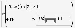
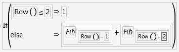
For example, the following formula calculates values for a column called Fib, which, after the formula is evaluated, contains the terms of the Fibonacci series (each value is the sum of the two preceding values in the calculated column).

The preceding formula uses the following functions: If, Row, Fib, and Subscript. As an exercise to become more familiar with these functions, create a Fibonacci sequence as follows:

   Name a blank data table column Fib.

   Right-click on the column header and select Formula.

   Select If from the Conditional Functions list.

   Select a<=b from the Comparison Functions list.

   Select Row from the Row Functions list.

   Select the second argument of the conditional statement.

   Type 2 and press Enter.

   Type 1 in the then clause of the If function and press Enter.

   Select the else clause of the If function.

   Click the + key on the keypad, type Fib as the first term, and then press Enter.

   Select Subscript from the Row Functions list.

   Select Row from the Row list, click the - key on the keypad, and then type 1.

   Repeat for the second term to add Fib with lag 2.

After you create the formula and click OK, the formula that you entered generates the values shown in Figure 4.6.

Figure 4.6 Results of the Formula Example

The Fibonacci sequence has interesting and easy-to-understand properties that are discussed in many number theory textbooks.

Using the Match Function

Conditional functions are commonly used to recode variables. If functions can be used for this, but you can also use the simpler Match function.

When you select Match from the Conditional menu, the Formula Editor shows a single Match condition with an empty expression and an empty then clause. The Match conditional expression compares an expression to a list of clauses. The condition then returns the value of the result expression for the first matching argument that is encountered. With Match, you provide the matching expression only once and then give a match for each argument.

For example, select Help > Sample Data Library and open Car Physical Data.jmp. The variable Type has five levels (Large, Medium, Small, Sporty, and Compact). Suppose that you want to combine Small and Compact into one category, Small/ Compact. In the Formula Editor of a new column, follow these steps:

   Select Match from the Conditional list.

   Select Type from the list of columns. The expr argument in the formula is populated.

   On the keypad at the top of the Formula Editor, click the Insert button three times.

   Type Small and Compact in the two value fields.

   Type Small/Compact in the two then clause fields.

   Click on the else clause field and select Type from the list of columns.

If the values in the Type column are Small or Compact, they are recoded as Small/ Compact. Otherwise, the new column is populated with the original values in the Type column.

As a shortcut, you can also auto-populate the Match conditional expression with the values for the variable.

   In the Formula Editor, select Type from the list of columns.

   Select Match from the Conditional list.

   Select Add Match Arguments from Data from the Match pop-up menu.

   Remove the arguments that you will not use, or click the Insert button to add new arguments.

Writing Match Statements with Recode

The Recode option in JMP provides an interface for recoding data and writing Match formulas. In this example, we use the Hollywood Movies.jmp sample data table. The file contains the Genre column, which has nine categories. Only two of the movies are in the Fantasy or Adventure genre. To combine these two genres, follow these steps:

   Select the Genre column in the data table.

   Select Cols > Recode.

   Click Adventure to select it.

   Hold down the Ctrl key and select Fantasy.

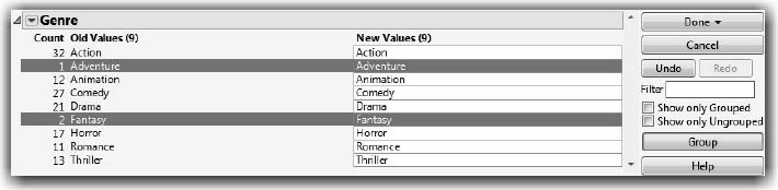
   Click Group.

   Change the new value to Fantasy/Adventure.

   Click Done and select Formula Column.

The new column with a Match formula is created.

Note: Recode provides many additional features for changing values in a column. Recoding is ideal for preparing categorical data for analysis.

Summarizing Data with the Formula Editor

The Formula Editor evaluates statistical functions differently from other functions. Most functions evaluate data only for the current row. However, all Statistical functions require a set of values upon which to operate. Some Statistical functions compute statistics for the set of values in a column, and other functions compute statistics for the set of arguments that you provide.

The functions with names prefaced by “Col” (Col Mean, Col Sum, and so on) always evaluate for all of the rows in a column. Thus, used alone as a column formula, these functions produce the same value for each row. You can add one or more grouping or By variables to the functions, which results in values for each combination of the By variables.

The other statistical functions (Mean, Std Dev, and so on) accept multiple arguments that can be variables, constants, and expressions.

The Sum and Product functions evaluate over an explicitly specified range of values.

The Quantile Function

The Col Quantile function computes a quantile for a column of n nonmissing values. The Col Quantile function’s quantile argument (call it p) represents the quantile percentage divided by 100.

The following examples are quantile formulas for a column named age:

Col Quantile(age, 1) finds the maximum age.

Col Quantile(age, 0.75) calculates the upper quartile age.

Col Quantile(age, 0.5) calculates the median age.

Col Quantile(age, 0.25) calculates the lower quartile age.

Col Quantile(age, 0.0) calculates the minimum age.

The pth quantile value is calculated using the formula I = p(N + 1) where p is the quantile and N is the total number of nonmissing values. If I is an integer, then the quantile value is y_p = y_i. If I is not an integer, then the value is interpolated by assigning the integer part of the result to i, the fractional part to f, and by applying this formula:

$$q_p=(1-f)y_i+(f)y_{i+1}$$

Note: To calculate a Quantile using New Formula Column from the data table, right-click on the column header and select New Formula Column > Aggregate > Quantile.

Using the Summation Function

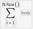
The Summation (Σ) function uses the summation notation shown here. To calculate a sum, select Summation from the Statistical function menu and create its argument. The Summation function repeatedly evaluates the expression for the index that you apply to the body of the function from the lower summation limit to the upper summation limit. The function then adds the nonmissing results together to determine the final result. You can replace the index i, the index constant 1, and the upper limit, NRow(), with any expressions appropriate for your formula.

Use the Subscript function in the Row function category to create a subscript for the body of the summation.

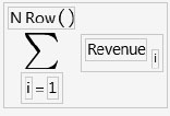
For example, the summation shown here computes the total of all revenue values for row 1 through the current row number. The function fills the calculated column with the cumulative totals of the revenue column.

Let’s see how to compute a moving average using the summation function.

   Select Help > Sample Data Library and open Current Stock Averages.jmp. Note that there is a column in the table called Moving Average. Use this column and its formula as a reference.

   Create a new column by selecting Cols > New Columns.

   Name the column Moving Average 2 and select Formula from the Column Properties list.

A moving average is the average of a fixed number of consecutive values in a column, updated for each row. The following example shows you how to compute a 10-day moving average for Close, the closing price of a high-tech stock. This means that for each row the Formula Editor computes the sum of the current Close value with the nine preceding values and then divides that sum by 10.

   Begin by selecting the conditional If function.

   With the If expression highlighted, select a>b from the Comparison function category, which is used to determine the row number value.

   For the left side of the comparison, select Row from the Row functions.

   Highlight the right side of the comparison and type 9. The If expression should now appear as Row()>9.

   Now highlight the then clause and begin the formula to compute the ten-day moving average by selecting the Summation function from the Statistical function category. Highlight the body of the summation and click Close in the columns list.

Now modify the summation indices to sum just the 10 values that you want:

   Highlight the summation body, Close.

   Select Subscript from the Row function category.

An empty subscript now appears with the summation body.

   To assign the subscript, either type the letter i, or drag the i from the lower limit of the summation into the empty subscript.

   Select the 1 in the lower summation limit and hold down the Delete key to change it to an empty term.

   Enter the expression Row()–9 inside the parentheses, using the Row selection in the Row function category.

   Click the upper index to highlight it and select Row from the Row functions.

To finish the moving average formula, you want to divide the sum by 10, but not start the averaging process until you actually have 10 values to work with.

   Click in the summation to highlight the whole summation expression.

   Click the divide operator on the control panel, and then enter the constant “10” into the highlighted dominator that appears.

   When you click Apply or close the Formula Editor, the Moving Average 2 column fills with values.

Now generate a plot to see the result of your efforts.

   Select Graph > Graph Builder, and drag Date to the X zone and both Close and Moving Average to the Y zone (at the same time).

   Right-click (or Ctrl-click on a Macintosh), and select Smoother > Change to > Line.

   Click Done and customize the graph as desired by changing the graph title, the orientation of the axes, and so on.

You then see the plot in Figure 4.7, which compares closing stock values with their ten-day moving average.

Figure 4.7 Plot of Close and Its Moving Average over Date

Generating Random Data

Random number functions generate real numbers by essentially “rolling the dice” within the constraints of the specified distribution. You can use the random number functions with a default “seed” that provides a pseudo-random starting point for the random series. You can also use the Random Reset function and give a specific starting seed. Figure 4.8 shows JMP’s extensive random number menu.

Figure 4.8 Random Functions Menu in Column Calculator

Each time you click Apply in the Formula Editor window, random number functions produce a new set of numbers. This section shows examples of three commonly used random functions, Uniform, Normal, and Column Shuffle.

The Uniform Distribution

The Random Uniform function generates random numbers uniformly distributed between 0 and 1. This means that any number between 0 and 1 is as likely to occur as any other. You can use the Random Uniform function to generate any set of numbers by modifying the function with the appropriate constants.

You can see simulated distributions using the Random Uniform function and the Distribution platform.

   Select File > New to create a new data table.

   Right-click (or press Ctrl and click) on Column 1 and select Formula.

   When the Formula Editor window appears, select Random Uniform from the Random function menu in the function list, and then close the Formula Editor.

   Select Rows > Add Rows and add 500 rows.

The table fills with random uniform values between 0 and 1.

Follow the same steps as before, except modify the Random Uniform function to generate the integers from 1 to 10 as follows.

   Select Cols > New Columns to create a second column.

   Click Random in the function list and select Random Uniform from its menu.

   Click the multiply sign on the keypad and enter 10 as the multiplier.

   Select the entire formula and click the addition sign on the keypad.

   Enter 1 in the empty argument term of the plus operator.

The next steps are the key to generating a uniform distribution of integers (as opposed to real numbers as in Column 1):

   Click to select the entire formula.

   Select the Floor function from the Numeric function menu.

The final formula is

Floor(Random Uniform()*10+1)

   Click OK to close the Formula Editor.

You now have a table template for creating two uniform distributions.

   Change the modeling type of the integer column to nominal so that JMP treats it as a discrete distribution.

   Select Analyze > Distribution, assign both columns to Y, Columns, and then click OK.

You see two histograms similar to those shown in Figure 4.9. The histogram on the left represents simple uniform random numbers, and the histogram on the right shows random integers from 1 to 10.

Figure 4.9 Example of Two Uniform Distribution Simulations

The Normal Distribution

Random Normal generates random numbers that approximate a normal distribution with a mean of 0 and variance of 1. The normal distribution is bell- shaped and symmetrical. You can modify the Random Normal function with arguments that specify a normal distribution with a different mean and standard deviation.

As an exercise, follow the same instructions described previously for the Uniform random number function.

   Create a table with a column for a standard normal distribution using the Random Normal() function.

The Random Normal() function takes two optional arguments. The first specifies the mean of the distribution; the second specifies the standard deviation of the distribution.

   Create a second column for a random normal distribution with mean 30 and standard deviation 5.

The modified normal formula is

Random Normal(30, 5)

Figure 4.10 shows the Distribution platform results for these normal simulations.

Figure 4.10 Illustration of Normal Distributions

The Col Shuffle Command

Col Shuffle selects a row number at random from the current data table. Each row number is selected only once. When Col Shuffle is used as a subscript, it returns a value selected at random from the column that serves as its argument.

For example, to identify a 50% random sample without replacement, use the following formula:

This formula chooses half the values (n/2) from Column 1 and assigns them to the first half of the rows in the computed column. The remaining rows of the computed column remain missing.

Initialize Data Options

When you add a new column to a data table, the Initialize Data menu in the Column Info window (shown in Figure 4.11) enables you to specify the type of initial data values for the new column. The default is Missing/Empty. The Random option populates the column with random data without accessing the Formula Editor or storing a formula in the column.

Figure 4.11 Initialize Data Options

Local Variables and Table Variables

Local variables let you define temporary numeric variables to use in expressions. Local variables exist only for the column in which they are defined.

To create a new local variable, use the button on the formula editor keypad. This button adds a temporary local variable to the formula editing area, which appears as a command ending in a semicolon. Alternatively, you can select Local Variables from the Formula Elements menu, select New Local, and complete the window that appears.

By default, local variables have the names t1, t2, and so on, and initially have missing values. Local variables appear in a formula as bold italic terms.

Optionally, you can create a local variable, change its name and assign a starting value in the Local Variable window.To use the Local Variable window, select Local Variables from the Formula Elements pop-up menu; select New Local, and complete the window, as illustrated here.

For example, suppose you have variables x and y and you want to compute the slope in a simple linear regression of y on x using the standard formula shown here.

$$\frac{\sum (x-\overline{x})(y-\overline{y})}{\sum {(x-\overline{x})}^2}$$

One way to do this is to create two local variables, called XY and Xsqrd, as described in the numerator and denominator in the equation above. Then assign them to the numerator and the denominator calculations of the slope formula. The slope computation is simplified to XY divided by Xsqrd.

The Local Variables command in the Formula Editor menu lists all the local variables that have been created.

Table variables are available to the entire table. Table variable names are displayed in the Tables panel at the left of the data grid. The Formula Editor can refer to a table variable in a formula.

Many of the sample data files have a table variable called Notes. The Table Variables command in the Formula Elements menu lists all the Table variables that exist for a table. You can create additional Table variables with the New Table Variable command in the Tables panel of the data table, or edit the values of existing table variables.

Working with Dates

Working with dates can present a challenge. Below are some frequently encountered example formulas involving dates.

Calculating Elapsed Time

Columns storing dates should be formatted as dates in the Column Info window. JMP dates are stored as the number of seconds since Jan 1, 1904. Creating the elapsed time in days (or minutes, hours, and so on) between two date-formatted columns requires the appropriate conversion formula. The formula shown here converts the elapsed time in seconds between Date 1 and Date 2 to days.

Age in Days

A variation of the elapsed time problem is calculating age (in days, minutes, and so on). This formula calculates the age in days between a date-formatted column and today using the Floor and Today functions.

Note: The Date Time Functions list in the Formula Editor provides a number of functions for working with dates. For example, you can use the Date Difference function to calculate the difference in two date-time values, using defined intervals (month, day, or hour).

Fixing Unformatted Dates

If dates have been entered into JMP in a character format, they can be converted to numeric date formats using a few key functions: Num, Word, and Substr (all under the Characters function group).

The formula shown above parses the character string and converts the dates in the Date column to a numeric format. Note that this formula returns values in “raw” format (number of seconds since Jan 1, 1904). Change the date format in the Column Info window to display as a date.

Tips on Building Formulas

Examining Expression Values

Once JMP has evaluated a formula, you can select an expression to see its value. This is true for both parameters and expressions that evaluate to a constant value. To do this, select the expression that you want to know about and right-click (PC) or Ctrl-click (Mac) on it. This displays a pop-up menu as shown here. When you select Evaluate, the current value of the selected expression shows until you move the cursor.

Cutting, Dragging, and Pasting Formulas

You can cut or copy a formula or an expression, and paste it into another formula display. Or you can drag any selected part of a formula to another location within the same formula. When you place the arrow cursor inside an expression and click, the expression is highlighted. When the cursor is over a selected area, it changes to a hand cursor, indicating that you can drag the highlighted formula under the cursor. As you drag across the formula, destination expressions are highlighted. When you release the drag, the selected expression is copied to the new location where it replaces the existing expression.

When you copy (or drag) an expression from one data table to another, JMP expects to find matching column names. If a formula column name does not appear in the destination table, an error alerts you when the formula attempts to evaluate.

Selecting Expressions

The Show Boxing red triangle option above the Formula Editor editing area tells JMP to outline terms within a formula. This outlining is called boxing.

You can click on any single term in an expression to select it for editing. You can use the keyboard arrow keys to select expressions for editing. You can also use the arrow keys to view the grouping of terms within a formula when parentheses are not present or the boxing option is not selected.

Once an operand is selected, the left and right arrow keys move the selection across other associative operands within the expression. The left arrow highlights the next formula element to the left of the currently highlighted term. The arrow also extends the selection to include an additional term that is part of a group.

Tip: Keep the boxing option on to see how the elements and terms are grouped in a formula that you create. It is often easier to leave the boxing option on while creating a formula.

The up arrow on your keyboard extends the current selection by adding the next operand and operator of the formula term to the selection. The down arrow reduces the current selection by removing an operand and operator from the selection.

Exercises

1.   The sample data table Pendulum.jmp contains the results of an experiment in a physics class. The data compare the length of a pendulum to its period (the time it takes the pendulum to make a complete swing). Calculations were made for a range of pendu- lums from short (2 cm) to long (20 m). Use the calculator to determine a model to pre- dict the period of a pendulum from its length.

(a)   Produce a scatterplot of the data by selecting Analyze > Fit Y By X and assigning Period to Y, Response and Length to X, Factor.

(b)   Create a new column named Transformed Period that contains a formula to take the square root of the Period column. Produce a scatterplot of Transformed Period vs. Length. Is this the graph of a linear function?

(c)   Try other transformations (for example, natural log of Period, reciprocal of Period, or square of Period) until the scatterplot looks linear.

(d)   Find the line of best fit for the linear transformed data by selecting Fit Line from the pop-up menu beside the title of the scatterplot.

(e)   This line is not the fit of the original data, but of the transformed data. Substitute a term representing the transformation that you did to linearize the data. For example, if the square root transformation made the data linear, substitute $\sqrt{\text{Period}}$ into the regression equation and solve the equation for Period.

A Physics textbook reveals the relationship between period and length to be $\text{Period}=\frac{2\pi }{\sqrt{g}}\sqrt{\text{Length}}$ where $g=9.8\frac{m}{s^2}$.

(f)   Create a new column to use this formula to calculate the theoretical values. Next, construct another column to calculate the difference between the observed values of the students and the theoretical values.

(g)   Examine a histogram of these differences. Does it appear that there was a trend in the observations of the students?

2.   Is there a correlation among the mean, minimum, maximum, and standard deviation of a set of data? To investigate, create a new data table in JMP with these characteris- tics:

(a)   Create ten columns of data named Data 1 through Data 10, each with the formula Random Uniform(). Add 500 rows to this data table.

(b)   Create four columns to hold the four summary statistics of interest, one column each for the mean, minimum, maximum, and standard deviation. Create a formula in each column to calculate the appropriate statistic of the ten data rows.

(c)   Select the Multivariate platform in the Analyze > Multivariate Methods menu and include the four summary statistics as the Ys in the resulting window. Pressing OK should produce 16 scatterplots. Which statistics seem to show a correlation?

(d)   As an extension, select two of the statistics that seem to show a correlation. Produce a single scatterplot of these two statistics using the Fit Y by X platform in the Analyze menu. From the red triangle menu beside the title of the plot, select Nonpar Density. Then select Save Density Grid from the menu beside the density legend.

(e)   Finally, select Graph > Scatterplot 3D and include the first three columns of the saved density grid. You should now see a 3D scatterplot of the correlation, which contains a peak where the data points overlapped each other. Use the hand tool to move the plot around.

3.   Make a data table consisting of 20 rows and a single column that holds the Fibonacci sequence (whose formula is shown on page 73). Label this column Fib.

(a)   Add a new column called Ratio, and give it the following formula to take the ratio of adjacent rows.

Note: This produces an error when evaluated for the first row. Click OK on the error window and resolve this issue.

$$\frac{Fib}{Fi{b}_{Row\left(\right)-1}}$$

What value does this ratio converge to?

(b)   A more generalized Fibonacci sequence uses values aside from 1 as the first two elements. A Lucas sequence uses the same recursive rule as the Fibonacci, but uses different starting values. Create a column to hold a Lucas sequence beginning with 2 and 5 called Lucas with the formula

$$\text{If}\left(\begin{array}{l}\text{Row}()==1\Rightarrow 2\\ \text{Row}()==1\Rightarrow 5\\ \text{else}\Rightarrow Luca{s}_{\text{Row}()-1}+Luca{s}_{\text{Row}()-2}\end{array}\right)$$

(c)   Create a column to calculate the ratio of two successive terms of the Lucas sequence in part (b). Is it the same as the number in part (a)?

(d)   Create a Lucas sequence starting with the values 1, 2. Calculate the ratio of successive terms and compare it to the answer in part (c).

(e)   There are innumerable other properties of the Fibonacci sequence. For example, add a column that contains the following formula, and comment on the result.

$${\displaystyle \sum _{\text{i}-1}^{\text{Row}()}\text{ArcTangent}\left(\frac{1}{Fi{b}_{2*\text{i}+1}}\right)*4}$$