Chapter 4 Data Modeling Described

4.1. Solution Modeling (Solution Model)

4.1.1. Business Concept Model

An overview of Business Concept Modeling was covered in Chapter 3. Now we’ll focus on the solution modeling activities:

4.1.2. Power of Dependencies

We cannot discuss data modeling without talking about normalization and functional dependencies. We already illustrated the mechanics of the process of normalization in chapter 2. The objectives of eliminating malformed relational data designs are (roughly) these:

• Reduce redundancy
• Avoid update anomalies
• Avoid information loss.

Working around these problems naturally leads to designing keys, which may be primary or foreign. But do we really need normalization and functional dependencies?

To get a feel for the approach that one could call “Relational Data Modeling Classic,” let us quickly review orthodox normalization by way of a famous example. This example appeared as a complimentary poster in the Database Programming & Design Magazine published by Miller Freeman back in 1989. The intellectual rights belong to Marc Rettig, now of Fit Associates. It is included here with his kind permission.

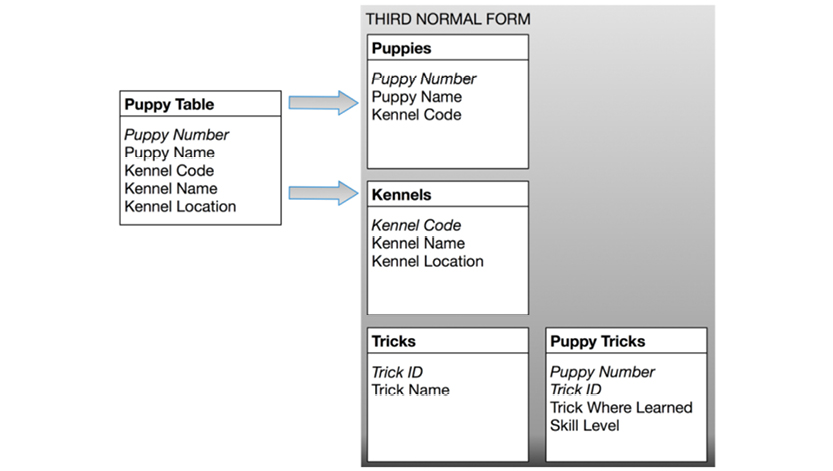
Although you cannot read the fine print, the facing page contains the poster in its entirety. Here are the 5 “Rules of Data Normalization” in a more readable fashion. The text here closely follows the text on the original poster.

RULE 1: Eliminate Repeating Groups

Make a separate table for each set of related attributes, and give each table a primary key.

Non-normalized Data Items for Puppies:

Puppy Number

Puppy Name

Kennel Code

Kennel Name

Kennel Location

Trick ID 1..n

Trick Name 1..n

Trick Where Learned 1..n

Skill Level 1..n

In the original list of data, each puppy’s description is followed by a list of tricks the puppy has learned. Some might know ten tricks, some might not know any. To answer the question, “Can Fifi roll over?” we need to first find Fifi’s puppy record, then scan the list of tricks at the end of that record. This is awkward, inefficient, and untidy.

Moving the tricks into a separate table helps considerably:

Separating the repeating groups of tricks from the puppy information results in first normal form. The puppy number in the trick table matches the primary key in the puppy table, providing the relationship between the two.

RULE 2: Eliminate Redundant Data

“In anything at all, perfection is finally attained not when there is no longer anything to add, but when there is no longer anything to take away.”

Saint-Exupéry, Wind, Sand and Stars

If an attribute depends on only a part of a multi-valued key, move it to a separate table.

Second normal form

In the Trick Table in the first normal form, the primary key is made up of the puppy number and the trick ID. This makes sense for the “where learned” and “skill level” attributes, since they will be different for every puppy/trick combination. But the trick name depends only on the trick ID. The same name will appear redundantly every time its associated ID appears in the Trick Table.

Suppose you want to reclassify a trick—give it a different Trick ID. The change needs to be made for every puppy that knows the trick! If you miss some, you’ll have several puppies with the same trick under different IDs. This represents an “update anomaly.”

Or suppose the last puppy knowing a particular trick gets eaten by a lion. His records will be removed from the database, and the trick will not be stored anywhere! This is a “delete anomaly.” To avoid these problems, we need the second normal form.

To achieve this, separate the attributes that depend on both parts of the key from those depending only on the trick ID. This results in two tables: “Tricks,” which gives the name for each trick ID, and “Puppy Tricks,” which lists the tricks learned by each puppy.

Now we can reclassify a trick in a single operation: look up the trick ID in the “Tricks” table and change its name. The results will instantly be available throughout the application.

RULE 3: Eliminate Columns Not Dependent on Key

If attributes do not contribute to a description of the key, move them to a separate table.

The Puppy Table satisfies first formal form as it contains no repeating groups. It satisfies second normal form, since it doesn’t have a multi-valued key. But the key is puppy number, and the kennel name and kennel location describe only a kennel (not a puppy). To achieve third normal form, they must be moved into a separate table. Since they describe kennels, kennel code becomes the key of the new “Kennels” table. The motivation for this is the same as for second normal form: we want to avoid update and delete anomalies. For example, suppose no puppies from the Daisy Hill Puppy Farm were currently stored in the database. With the previous design, there would be no record of Daisy Hill’s existence!

RULE 4: Isolate Independent Multiple Relationships

No table may contain two or more 1:n or n:m relationships that are not directly related.

Rule Four applies only to designs that include one-to-many and many-to-many relationships. An example of one-to-many is that one kennel can hold many puppies. An example of many-to-many is that a puppy can know many tricks, and many puppies might know the same trick.

Suppose we want to add a new attribute to the Puppy Trick table: “Costume.” This way we can look for puppies that can both “sit up and beg” and wear a Groucho Marx mask, for example. Fourth normal form dictates against using the Puppy Trick table because the two attributes do not share a meaningful relationship. A puppy may be able to walk upright, and it may be able to wear a suit. This doesn’t mean it can do both at the same time. How will you represent this if you store both attributes in the same table?

RULE 5: Isolate Semantically Related Multiple Relationships

There may be practical constraints on information that justify separating logically related many-to-many relationships.

Usually, related attributes belong together. For example, if we really wanted to record which tricks every puppy could do in costume, we would want to keep the costume attribute in the Puppy Trick table. But there are times when special characteristics of the data make it more efficient to separate even logically related attributes.

Imagine that we now want to keep track of dog breeds and breeders. Our database will record which breeds are available in each kennel. And we want to record which breeder supplies dogs to those kennels. This suggests a Kennel-Breeder-Breed table which satisfies fourth normal form. As long as any kennel can supply any breed from any breeder, this works fine.

Now suppose a law is passed to prevent excessive arrangements: a kennel selling any breed must offer that breed from all breeders it deals with. In other words, if Kabul Kennels sells Afghans and wants to sell any Daisy Hill puppies, it must sell Daisy Hill Afghans.

The need for a fifth normal form becomes clear when we consider inserts and deletes. Suppose a kennel decides to offer three new breeds: Spaniels, Dachshunds, and West Indian Banana-Biters. Suppose further that it already deals with three breeders that can supply those breeds. This will require nine new rows in the Kennel-Breeder-Breed table—one for each breeder/breed combination.

Breaking up the table reduces the number of inserts to six. Above are the tables necessary for fifth normal form, shown with the six newly-inserted rows in bold type. If an application involves significant update activity, fifth normal form can save important resources. Note that these combination tables develop naturally out of entity-relationship analysis.

This is the end of the text from the original poster.

The normalization approach is an example of what happens when one particular scenario is generalized. The assumption being that table design is made from a long list of fields in no particular order. If, on the other hand, the table is based off a structural analysis (like an entity-relationship analysis), there shouldn’t be any need to normalize. Instead the structures should be visualized as part of the analysis. You, then, should have no problems deconstructing a graph-based data model (which is what entity-relationship models are all about) into a table-based data model.

Let us turn to the benefits of working with dependencies, staying in the puppy context.

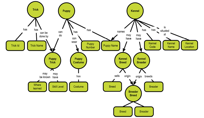
As argued earlier regarding the relational model, things would definitely be easier if the starting point were not a list of fields, but instead a concept map:

Remember that the way we arrive at a concept map like the above is based on the semantics (meaning) of the linking phrases. Some linking phrases determine a simple dependency (like “has”) on the unique identification of the object it is a property of. Other linking phrases contain action verbs meaning that they signify intra-object relationships (like puppy can do puppy trick).

So let’s work through the process described earlier, from the poster:

Eliminate repeating groups? Not relevant. We already identified them by way of the arrowheads on some of the relationships.

Eliminate redundant data? Not relevant, since a property belongs to one object only, and is identified by its identity.

We will group the properties into tables, if we want to use tables at all. Composition from a well-structured starting point is a whole lot easier than decomposition of a semantically-blurred bunch of data.

Eliminate columns not depending on the key? Not relevant, for the same reason as above.

Isolate independent multiple relationships? Easy. We would add a new object, puppy costume, with a property named costume. We would point at it from the puppy trick, just as in Marc Rettig’s example. Here it is:

Isolate semantically related multiple relationships? Again, easy. Follow basically the same logic as above. Just as for entity-relationship modeling, as Marc Rettig comments, our concept map or our logical model will naturally show the relationships. Here it is in fifth normal form (5NF):

It is obvious that depicting the dependencies as a directed graph gives a deep understanding of the functional dependency structure. There have been only a few attempts at incorporating directed graphs over time:

• Graph Algorithms for Functional Dependency Manipulation by Giorgio Ausiello, Alessandro D’Atri and Domenico Sacca, Journal of the ACM, NO. 10/1983
• The predecessors of the NIAM / ORM Object/Role Modeling paradigm based on Professor Nijssen’s work at Control Data in Brussels in the 1980’s.

Unfortunately, visual dependency analysis never took off in the 1980’s. This was most likely due to the mathematical twist inherent in traditional normalization. Most people were busy implementing SQL and data models soon reflected that the universe of discourse was set to be tables and foreign keys for many years. Only the NIAM / ORM practitioners carried on using their highly visual approach to modeling.

Given that graph visualization is the way forward (as argued so far in this book), is there anything we can carry forward from normalization?

The answer is simple: identity and uniqueness. These two things contribute hugely to setting the context in precise ways. We will come back to this in the section about identifiers, keys, and pointers.

If winding up with a relational data model in the end is not a requirement, you experience more freedom to direct your model design more toward the semantics and reality of business. Do not produce a relational model, if relational is not a requirement.

Aside: Many of the troubles in relational models could have been avoided, if SQL had contained support for dependencies. Let us see, what that could have looked like.

Think of the classic table, Order_Details, as it could be defined in SQL:

CREATE TABLE Order_Details (

  OrderID number NOT NULL,

  ProductID number NOT NULL,

  UnitPrice number NOT NULL,

  Quantity number NOT NULL,

  Discount number NOT NULL,

  CONSTRAINT PK_Order_Details PRIMARY KEY

  (

    OrderID,

    ProductID

  ),

  CONSTRAINT FK_Order_Details_Orders FOREIGN KEY

  (

    OrderID

  ) REFERENCES Orders (

    OrderID

  ),

  CONSTRAINT FK_Order_Details_Products FOREIGN KEY

  (

    ProductID

  ) REFERENCES Products (

    ProductID

  )

);

Imagine for a few moments that the fathers of relational and SQL got carried away and “materialized” dependencies in more explicit ways:

CREATE TABLE Order_Details (

  FOREIGN KEY OrderID NOT OPTIONAL

    DEPENDENCY Order_consists_of

    REFERENCES Orders (OrderID),

  FOREIGN KEY ProductID NOT OPTIONAL

    DEPENDENCY Products_ordered

    REFERENCES Products (ProductID),

  PRIMARY KEY PK_Order_Details

    (OrderID,

    ProductID),

  PROPERTY UnitPrice number NOT OPTIONAL DEPENDENCY has_Price,

  PROPERTY Quantity number NOT OPTIONAL DEPENDENCY has_Quantity,

  PROPERTY Discount number NOT OPTIONAL DEPENDENCY Discount_given,

);

Except for the primary key (identity and uniqueness constraint, really), it’s all dependencies of either the relationship type or the functional dependency (or primary key) type. Clearly this is much more informative than the relational offering.

End of aside.

Another little aside: Actually dimensional modeling is more interesting than ever. There are definitely good reasons to think in terms of dimensions and facts (or “events”). The granularity of dimensions sets the context of the event. And context is another way of saying “multidimensional coordinates,” or “landmarks,” in the information “landscape.” Event-driven modeling is a very productive way to look at how best to describe business processes.

But first, some practical pieces of advice for preparing a solution data model based on user stories expressed as concept maps.

4.1.3. Names Matter

The transition from concept map to solution data model is somewhat mechanical, as you will see below. Before we get into that, though, we need to reemphasize some things.

Since in some cases the physical data models may be schema-less or schema-on-read, we need a layer of presentation for the business users. That layer is our solution data model.

Furthermore, much of the big data that people want to analyze is more or less machine-generated or system-generated. Again, this calls for a user-facing data layer toward the analytics environment.

Finally, even in integration projects (including most of data warehousing and business analytics), consensus on business names is what is needed to obtain acceptance in the business user community. Names include object type names, property names and relationship names (“linking phrases,” in concept-speak).

Relationship names are important because they also are used to infer the type of the relationship (or dependency). Action verbs indicate activity on business objects, whereas passive verbs (like “has”) indicate ordinary functional dependencies between an identifier of a business object type and its properties.

Relationships are bidirectional, since they can be read in two ways:

For those reasons, names matter. However, I tend only to write the name coming from the “parent.” That would be “has” in this case, since the relationship is one-to-one and left-to-right ordering is applied. The key point is that some linking phrases (the names of relationships, in concept mapping terminology) contain verbs, which imply that somebody or something “makes something happen.” In other words, the relationship denotes something which is more than a plain property depending on the identity of something. This makes the target a candidate for being identified as a business object type.

Concepts should also be backed up by solid definitions wherever there is risk of ambiguity. Definitions of core business concepts often persist for a long time and reach many people. This means that they should not only be precise and concise, but they should also be easily communicated and easily remembered. In many respects, production of good definitions is a skill that requires concentration and attention. For world class expertise on good definitions, read this excellent book: “Definitions in Information Management” (Chisholm 2010).

Names should be as specific as they can get. Avoid “Address,” if what you are talking about is “Delivery Address.” It’s always a good idea to consult with a subject area expert to make sure names make sense and are consistent with the business’ terminology, before proceeding with the model.

4.1.4. Finding Patterns

Another thing to consider before materializing the solution data model is patterns. Many kinds of business activities and business objects have been defined as best practice data models. It is worth reading David Hay’s fine collection of data models in his book, Enterprise Model Patterns, Technics Publications (May 15, 2011) [8].

Looking at the last version of the Puppy Kennel concept map, we realize that we need a pattern:

The kennel location property seems a bit un-modeled, if you ask me. Well, Kennels have business addresses, and David Hay has several pages about addresses and geography in his data model patterns book [8].

How did we notice that something was missing about Kennel Locations? Because the linking phrase contains an action verb (situate). Action verbs tend to denote relationships between two object types, not between objects and their properties. So, that will be another item to check on before transforming to a solution data model.

4.1.5. Cardinality and Optionality

It can be argued that the issues of cardinality and optionality are coupled to the physical data store (at least in the sense of representation of missing matches). In SQL, this is the crux of the good old “NULL-debate.” I tend to stay away from using NULLs. I spend most of my time in data warehouse models, where default values are a recognized practice.

Cardinality is defined in Wikipedia like this:

In the relational model, tables can be related as any of “one-to-many” or “many-to-many”. This is said to be the cardinality of a given table in relation to another. For example, consider a database designed to keep track of hospital records. Such a database could have many tables like:

a doctor table with information about physicians; a patient table for medical subjects undergoing treatment; and a department table with an entry for each division of a hospital.

In that model:

• There is a many-to-many relationship between the records in the doctor table and records in the patient table because doctors have many patients, and a patient could have several doctors;
• There is a one-to-many relationship between the department table and the doctor table because each doctor may work for only one department, but one department could have many doctors.
• A “one-to-one” relationship is mostly used to split a table in two in order to provide information concisely and make it more understandable. In the hospital example, such a relationship could be used to keep apart doctors’ own unique professional information from administrative details.

https://en.wikipedia.org/wiki/Cardinality_(data_modeling)

For cardinality, it is good to know whether a relationship is:

• One-to-one or zero/one to zero/one (1:1)
• Zero/one to zero/many (1:M)
• Zero/many to zero/many (M:M).

The 1:1 relationships can be visualized as connections without arrowheads:

The 1:M relationships can be visualized as a connection with one arrowhead:

The M:M relationships can be visualized as a connection with an arrowhead on both sides.

I do not recommend visualizing the starting or ending point as being capable of being “empty.” This is, in essence, more related to optionality, which varies across data stores. The matter of optionality is close to being a business rule, which I generally prefer to treat as a layer on top of the data model.

I do recommend that a document be created (and kept up to date) to contain the business-level rules (for things such as optionality and default values), where applicable.

At the physical modeling level, these cardinality issues should, of course, be resolved in a way that matches the capabilities of the platform.

“Optionality” is concerned with the “zero” cases in the cardinalities listed above. Consider 1:M:

• What happens if there is nothing on the “1” side? A doctor not being placed in any department, currently, for example, or
• What happens if there is nothing on the “M” side? A department without doctors, for example.

In SQL there is a much debated “null” value construct. A “null” represents “nothing here”. I do prefer using default value schemes over using SQL-nulls. There are many articles about this, not least from the Kimball Group. Topics include:

• Keeping “dummy” records available and letting them participate in hierarchies, etc. (It can be useful to report numbers on “unknown” levels.)
• Using at least an “Unknown“ or “Not specified” approach for missing information (if in SQL).
• Using default low and high dates for missing dates.

4.1.6. Housekeeping

It’s best practice to keep order in your own database through accountability. It’s important to keep track of who did what and when. It is prudent to keep track of at least these pieces of metadata, for all object types:

• Who created this record?
• When was the record created?
• Who most recently changed this record?
• When was the date and time of the most recent change?

If you are in a data warehouse context (or other data integration contexts), you might also like to include technical metadata about the ETL processes, including:

• Which process loaded this record?
• When was the record loaded?
• What was the source system of the record?
• Versioning control dates (from and to).

4.1.7. Modeling the Subject Area Overview

You’ll frequently create a high-level concept map to provide an overview of a subject area. This one is for a car dealership, drawn from my first book [5]:

Notice how the upper levels are mostly classifications and other hierarchies. The levels in the middle are the core business objects engaged in the business processes. The concepts at the lowest level are all business events or other records, some of them of the “snapshot” type (like inventory on a given date). Also note that the concepts on the lowest level are actually the “value chain” of the business, starting with budget, flowing over procurement to inventory and sales, and later, maintenance and profitability.

Obviously there should be no “islands,” as everything should be connected to something. Once you get into looking at properties, the solution data model will become clearly visible; concepts which carry properties are business objects, whereas concepts without properties are probably just abstractions (which you may wish to get rid of, or describe with properties, as appropriate).

This type of overview will give you a head start on building a solution data model. Invest a few hours in creating such an overview, get it approved by the business people, and let it guide the rest of the modeling activities.

4.1.8. Data Types

If you have not already done so (at the level of concept map or definitions document), now is the time to think about the business level data types. Choose simple types like amount, integer, number, date, or string. Prepare yourself for surprises, though. Consider representation of large numbers, high precision, dates, and timestamps.

On the other hand, physical data types can wait until you complete the physical implementation model. At the physical level, you could have the full palette of data types, including things like Apache AVRO and JSON.

Graph databases (and many other NoSQL data stores) are schema-less or based on “schema on read,” meaning that the data “tells the consumer what they are”. There are plenty of ways of doing this, but as it turns out, there is metadata somewhere. Maybe the understanding is inside one application only, and maybe there is a metadata catalog in the system. Whichever way, you run into, a structure model of the data as it gives meaning to the business is indeed still necessary.

The real world is kind of messy and half-structured anyway. Forcing that reality into a relational schema, which is hard to maintain, is not the best idea. In relational solutions, that means lots of sparse tables (empty fields) and the infamous complexity of null-handling. That can be avoided in some of the newer technologies, at the expense of higher read-time processing complexity.

4.1.9. Identifiers, Keys, and Pointers

The days of analyzing functional dependencies (such as looking for foreign keys) are now behind us. The rationale for relational normalization was not clearly stated from a business perspective, but the benefits were clearly related to identity and uniqueness.

These issues are at the level of the solution model. But why do we need to worry about this? The trouble is that we humans do not really care about uniqueness. What is in a name, anyway? We all know that “James Brown” can refer to a very large number of individuals. The trick is to add context: “Yes, you know, James Brown, the singer and the Godfather of Soul.” When uniqueness really matters, context is the definite answer.

The requirement for unique identification is, then, an IT-derived necessity. This gave rise to the “artificial” identifiers (Social Security Number, for example) on the business level and the ID fields on the database level. We, as data modelers, must handle these difficult issues in a consistent manner across:

• Identity
• Uniqueness
• Context.

This reflects the observation that cognition is based on “location” in the meaning of “multi-dimensional coordinates.” Uniqueness is based on the very same thing.

The end result is that identity is functionally derived from uniqueness, which sets the context. This is the foundation of the commonly discussed “functional dependencies” in relational modeling, including the whole of normalization, candidate keys, primary and foreign keys and what have you.

The relational discussion started sort of backwards. Much of the discussion about candidate keys is based on the assumption that the problem to be solved is structured as follows:

• Here is a relation (or a relvar, strictly speaking) having these attributes (S#, SNAME, etc.).
• What could possibly be the candidate keys?
• What is the quality (uniqueness, I guess) of those keys?

But that is a very awkward starting point. Why pick that particular permutation, out of all the attributes that could eventually contribute to a “well-formed” (normalized) relation (relvar)?

Why not look at context, which for us visual modelers is “business as usual.” Let us try doing just that. We will revisit the Puppy / Kennel example as it existed at step 4 (4NF). Identity is really the scope of properties. If we look at skill level and where learned, we can see their scope:

Skill level shares scope with where learned, and both are driven by the identity of the puppy trick. For now, we need to establish a reliable identity of puppy trick. This used to be referred to as “finding the primary key,” but I propose we get away the term “keys,” since that terminology is closely related to normalization, which is not so relevant anymore.

Uniqueness is the matter of identifying what (on the business level) makes an identity unique. If you are a data modeler, you will not be surprised by the uniqueness behind puppy trick:

Yes, the puppy trick is uniquely defined by the combination of trick and puppy (i.e. whatever their identities are defined as). Enforcing uniqueness is also an important task in the design of a solution data model. (Previously this was called “foreign keys”, but we’ll abandon that term too.)

There are no good reasons for adding visual “icons” or special markers, because the uniqueness is implied by the structure. Painting the uniqueness blue wasn’t even completely necessary.

Identity determines the scope of a property. Skill level, for example, applies to puppy trick since it is the skill of that Puppy in performing that Trick. Puppy Trick is really a M:M relationship with a few properties attached. The identity of Puppy is simpler, it is the puppy number, which we have designed and introduced with the purpose of representing the identity of the Puppy.

Uniqueness determines the business level criteria for ensuring uniqueness in the database. Puppy trick is unique across the combination of the identities of trick and puppy. Note that uniqueness is always based on the identities and that the representation of the identities may change over time (being redesigned for some reason). In that way, uniqueness is more like a rule, while identity is a representation of something that we use to identify occurrences of business objects in the real world.

Note that so far we are talking business level. Once we get to the solution design we will start to mess around with IT-generated keys and so forth.

Let us work our way through a somewhat larger example. It originates in the work of Peter Chen in 1976, but I have worked a bit on the concept names to make them more business-like and precise. Back then it was simply called the COMPANY database. The task at hand is to establish the identities and uniqueness criteria of the concepts contained in the concept model.

First of all, let us look at the example as a naive concept map:

Only one assumption has been made: The manager-related relationship between employee and department is by definition a one-to-one relationship. (And, of course, that departments without managers are not allowed.)

The first step is to check all dependencies (relationships between properties of objects) and identify those properties (remove the arrowheads):

Note that address, department location, and project location very well could have been business object types of some address/geolocation pattern(s). But the data modeler made the business decision that there is no need to keep detailed structures for those fields, since a simple text string will do. This is an example of generalization for simplicity at work.

Also notice that two new concepts have emerged:

• Manager start date is now a property of the new concept of department manager. This change brings clarity and straightforward modeling.
• Hours spent is now a property of the new concept of project work for the same reasons as above.

Finally, the modeler has left the self-reference “supervises” untouched for now.

The next step is to look for natural identities (natural keys / business keys). Before we do that, we’ll make another tweak to the example. Using Social Security Numbers (SSNs) are not advisable in Northern Europe (where I am from). For this reason, we’ll make SSN an optional alternate key (or search field) and invent an employee number to handle the identity of each employee. This change is reflected here:

After our slight modification, we can find three natural identity-setting fields (keys, if you insist), and we marked them in bold:

• Employee number (with Social Security Number as an optional alternate)
• Department number
• Project number.

Dependent name is also highlighted, but is has some problems, which we will come back to.

In general, inventing new natural identities can be very practical for us in IT. We have been the ones driving that trend over the years. Business people do not object too much, and at times they can see why such keys are practical.

Dependent really does not have a natural identity. We know that the dependents are depending on an employee, so employee number will be a part of the identity of dependent, but we would like to know more than that. Dependents are clearly “objects” in their own right, by all definitions. It would be tempting to ask for Social Security Numbers, but that is not a path that the business wants to enter. Dependent name is not guaranteed to be unique. We must solve this in our scheme for identity and uniqueness in this model.

Project work and department manager will have composite keys matching the identities of their respective dependency originators. So, we will go forward with the three natural identities we discussed (Employee Number, Department Number, Project Number):

What does this imply for identity and uniqueness? From the diagram above, you can easily see:

• The uniqueness of an object or property is determined by the relationships coming to it from the concepts “higher up”
• The identity of an object is thus the same as the combined identities of the referencing concepts
• Properties, on the other hand, share the identity of the object that they are depending on (which is the defining criterion of a property).

Using these simple “visual inspection” methods, we are able to conclude the context and hence the uniqueness of each object type:

Object type	Identity	Uniqueness
Employee	Employee number	Employee number
Department	Department number	Department number
Project	Project number	Project number
Department manager	Department number + Employee number + Manager start date	Department number + employee number + manager start date
Project work	Project number + Employee number	Project number + employee number
Dependent	Employee number + “something”	?
Supervises?

Notice the composite identities of department manager and project work. Department manager’s uniqueness will allow for a time series of successive department managers. But project work’s uniqueness will only allow for accumulating hours spent.

4.1.10. Keys

As modelers, we are allowed to invent things. One category of creativity is known as “keys.”

Working with large concatenated keys, for example, is really not very practical. We much prefer the precision of unique, simple (i.e. one variable) fields. This was first established in 1976, in an object-oriented context. It soon came to rule the world of primary and foreign keys, under the name “surrogate key.”

It turned out that business-level keys were rarely single-level fields (unless they were defined by organizers building IT-style solutions). Think account numbers, item numbers, postal codes, and the like. Even if reasonably precise concepts were used, they were not always guaranteed to be unique over a longer period of time. Item numbers, for instance, could be reused over time.

This is why surrogate keys became popular. I have done a lot of modeling in data warehouse contexts and I know from experience how volatile things (even business keys) can be. This is why I recommend always using surrogate keys as a kind of insurance. Non-information-bearing keys are quite practical. Generating them (large integer numbers, for example) is up to the physical platform. But the rule is that the surrogate key should match the uniqueness criteria.

Surrogate keys should be kept inside the database and should not be externalized to business users, but we’ll put them into the diagram for now.

Note how the appearance of physical-level identity insurance (via the surrogate keys) can help us solve the two remaining modeling problems that we had:

“Supervises,” which looked a lot like a pointer, can now be implemented as a second surrogate, “supervisor ID,” which points to the employee that supervises this employee.

And we can now generate a dependent ID. The business rule for uniqueness could be that the employee number plus dependent name should be unique, and will therefore generate a surrogate key. But this is a business decision; it can be verified in the data, if available already.

The diagram above is a solution-level concept map that includes an identifier (Xxxxxxx Id) for each object type. The nature of the identifier is implementation-specific, with regards to the physical platform chosen later on. But the purpose of the identifier is to serve as a simple, persistent, unique identifier of the object instances. (This is, after all, the nature of a surrogate key.)

Finally, we can compress the diagram into a property graph, which looks like the model on the facing page.

Notice the “employee home address.” In the concept map, it was only “address,” but the linking phrase was “employee lives at address.” In order not to lose information when removing the linking phrases, it is highly recommended to carry non-trivial information over into the property names.

4.1.11. Handling Time

Dates and times are some of the toughest challenges in databases. We have struggled with them since the 1970s. Date and time are mixed into a variety of data types, in many data stores and DBMS products. Some types can be:

• Pure date
• Date and time in one property
• Time in its own property.

Dates and times obey some slightly irregular international rules set for the management of time zones, as you know. They are not systematic in the sense that they can be derived from the value of something. For examples, look up the time zones in and around Australia and the Pacific Islands.

Calendars are somewhat easier, but still subject to a lot of national and cultural variations. Here is a plain US calendar:

Even though there are only two special days, the calendar above does not apply outside of the US. Valentine’s Day has found its way into Europe, but there is no Presidents’ Day. US National holidays are not business days in the US, but they may well be so in other countries. If your data model is required to support global operations, you must cater for this in all date-related logic. You might also need at least four variables on everything:

• Local date (pure)
• Local time (no date involved)
• Global date (pure)
• Global time (set to GMT, for example).

Be mindful of which server you pull the date and time information from. Much depends on the settings of those servers and database instances.

Another issue is the handling of missing dates. If you want to avoid nulls (and who doesn’t?), you could define default low and high dates, which are supplied whenever a date (or time of day) is missing. Sometimes we record future dates on records, which are known to us now, but where the event is still to happen within a few years, maybe. The future date could be fixed, like for a date of a dividend payment. But occasionally the future date is not known at this time. This is not very elegant modeling, but it happens in the real world; the consequence is having to define a “future undefined date” (which could also be the general value of a default high date that you have chosen).

On the business level, dates and times serve the purposes of pinpointing the date and time of both events (e.g. sales transactions) and “snapshots” (e.g. inventory counts). A series of transactions is a classic timeline record of events:

In the data warehousing world, a date/calendar dimension is a given requirement. If your operations are multi-national, you might need several calendars. Just as reporting and analytic applications need to know about calendars (e.g. public holidays, banking days), ordinary applications need to keep track of several properties of dates and times. Prepare accordingly.

Sometimes you have to handle state changes. In the financial world, for example, buy/sell transactions in securities can be in one of several states at any given time. Over time they ascend raised up through a hierarchy states much like this:

• Considered
• Planned
• Agreed
• Preliminarily booked
• Settled
• Finally accounted for.

That means that the same transaction exists in different versions throughout its lifecycle. Date and time are necessary to keep track of these different versions.

This brings us to versions in general.

Not only in data warehouses, but certainly also in other kinds of applications, version control is a requirement. Generally, the requirements are on the level of:

• Which version is current?
• What is the starting point and ending point of a given version (with date and/or time precision)?
• When did this version come into existence?

Sometimes backdated corrections are necessary. This could involve, for example, correcting a price which was found to be wrong at a later point of time:

Obviously, keeping two versions depends on accounting practices and possibly also regulatory requirements. Check carefully with someone familiar with business rules and requirements to determine your particular situation.

If you are into versioning, you could consider modeling concepts as chains of events. For instance: “The next event following this version of this transaction is XXXXX on date YYYYMMDD.” Graphs are excellent for modeling and implementing these. You might also be interested in prior event chains. For instance: “The event that preceded this version of this transaction was XXXXX on date YYYYMMDD.”

4.1.12. Design Involves Decisions

Never forget that data modeling is design! Design means making decisions—decisions that impact the business quality of the solution.

If you haven’t noticed by now, we often encounter a dilemma between supporting the business, with its processes and questions (both present and future), and keeping things simple. A balanced solution is what we should strive for.

Note that the conceptual model, if you have one, is often very liberal regarding dependencies and other structural issues. You do have to keep an eye on the structure (which is inherent in the data), once you get around to modeling it.

We do have some generally applicable “designer tools” in our mental tool belt:

• Abstraction, i.e. generalization and specialization, a.k.a. aggregation
• Classification and typing
• Life-cycle dependencies and versioning
• Recognizing hierarchies.

There are also some problem areas to be aware of:

• One-to-one relationships
• Many-to-many relationships and nested object types
• Trees (hierarchies of different kinds).

We’ll examine these issues in the following sections.

In general, generalization involves making things more widely usable—expanding the applicable context. But specificity strengthens the comprehension of that particular context.

In chapter 6 we will delve into some of these issues. Here are some helpful tips to get you started:

• Do not force business objects into relationships.
• Be careful with understanding linking phrases (verbs are good indicators of relationships).
• If you’re not sure whether something is a property or a relationship, check the verbs!
• Do not use composite values (repeating groups).

Good craftsmanship means that what you build lasts a long time. Think about what the data model can be used for—both now and in the future. Try to make it more widely accessible, but do not generalize it ad absurdum.

Also consider the lifespan of the terminology and concepts used. Will they last long enough? Will they be understood by business users coming on board five or ten years from now?

And remember that design decisions impacts the business. Ensure proper acceptance from those folks, before you force them into something that they find awkward or downright wrong. Acceptance can be a nod of the head or also a formal sign-off event at the other end of the formalism scale.

4.1.13. Abstraction, Specialization, and Generalization

Abstraction is the strongest problem-solving weapon in your arsenal as a data modeler. Abstraction involves creating layers:

Here you can “generalize” circles, rectangles, and triangles to be shapes. Or you can “specialize” shapes into being circles, rectangles and triangles. Moving up to a higher level layer is generalizing, and specializing involves working your way down into more and more detail.

Generalization generally makes things more broadly useful; at the same time, some details are sacrificed. Specialization, on the other hand, gets you more detail and more complexity. Make sure to consult your business contacts about how much specialization (or lack thereof) they really want and need. Another way of expressing this is with terms like “supertypes,” “subtypes,” and the like. If you’re using that terminology, the question to ask becomes: “Do we want the subtypes to be materialized in the solution model, or not?” One key issue, of course, is what to do with subtype-specific properties.

As background for the discussion, here is a concept model of a subset of FIBO (Financial Industry Business Ontology), which is described further in section 5.4. The conceptual level is carefully modeled and described in the semantic web standards OWL and RDF, so every detail about subtypes and all of the rest are fully documented. I have simplified matters a bit to look like this:

Here we will look at specific issues related to our discussion about abstractions. First of all, there are an abundance of “independent parties” at the top of the concept model:

In fact, “central bank” is also a subtype of independent party (of the type monetary authority). All of the parties have very similar attributes, inherited from a “formal organization” supertype. We will therefore generalize them into one type of business object, called “party.” This kind of “player / agent” generalization is quite common; it has both advantages and disadvantages. Here we prioritize simplicity so that party gets all of the relationships:

• Regulates (currencies, accomplished by central banks)
• Market data provider
• Publisher
• Authority (either an authorized independent party or a monetary authority).

To keep the information about the important subtypes (which we have eliminated via generalization), we have introduced a couple of categorizations into the solution model at the party level:

• Monetary authority (yes or no)
• Interest rate authority (yes or no).

They are just properties, though, at the party level:

Notice that the concept “Published Financial Information” is really just a categorization of market rate and economic indicator. From a practical point of view, it does not garner a whole lot of information; as such, and it is ignored in the solution data model.

Looking at the full concept model above, you will notice that “market rate” only carries one property: volatility. To maintain it as a separate level seems like overkill, so we will introduce a little bit of redundancy and push it down to the subtypes of market rate. Such “pushing down” is quite common. In our case, it is perfectly acceptable because volatility is dependent on the rate at the given point of time; you will only find this at the lowest level of the rate subtype instances, anyway. The FIBO conceptual model is not really concerned with how to handle time-series data; it focuses mostly on the concept level.

The solution data model will pretty much follow the structure of the concept model, as you can see in a first approximation here:

The properties shown in the concept model above will be placed on the lower level (containing rate business object types). More on this in chapter 5.

4.1.14. Unusual Concepts

Sometimes you may run into “unusual concepts,” which must be handled in unique ways. One of the scenarios is the “nested object types,” a term used in the context of fact modeling. Here is a naive representation of one such example:

Students enroll in courses, and each enrollment results in a rating. Basically, this is a ternary relationship—there are 3 participating concepts. Notice that the resulting relationship is of the arrow-less, one-to-one type; it emerges from the many-to-many relationship between students and courses.

One good way to visualize this is by taking advantage of the property graph model’s ability to have properties on relationships:

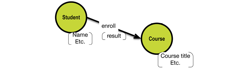
This works well if your final destination is a property graph database (such as Neo4j). However, it your target is a SQL database, you will most likely end up having three business object types:

In my opinion, the representation of three object types is fair and to the point. Enrollments do happen and are rather important business events, which makes them emphasized in the data model.

In fact, there is almost always a real business object behind a many-to-many relationship. In “Kimballian” (multidimensional) data modeling, there is a construct called the “factless fact”: a fact table without any other information beyond the foreign keys to the dimensions.

Such a table is the “mother of all relationships.” In fact (pun intended), even factless facts most often have properties (or measures), once you start looking for them.

Another common use of properties on the relationship level is “weight.” This could signify, for instance, participation or part-ownership. This could certainly be implemented as a property on an edge in a property graph, but in most peoples’ minds, a business object type like “partition” would make the most sense. This brings us back to having something substantial in a many-to-many relationship: In the example above Enrollment is a many-to-many relationship between Student and Course. And Enrollments carry information such as dates.

Another odd fellow is the one-to-one relationship. Between object types and their properties there are always one-to-one relationships—they’re also known as dependencies. But one-to-one’s do occasionally arise between business object types. Most instances occur in the realm of business rules. Here is one example:

(Remember that the relationship is “read” in a left-to-right order.)

Having only one insurer per insuree would be a bit impractical. In real life, most of us have different insurers for different assets (auto insurance, health insurance, etc.).

Self-references also crop up in data models from time to time. Here is a simple example that we saw earlier:

It is worth checking whether the relationship is information-bearing. That could well be the case, like in this example:

This, by the way, once again confirms the assumption that many-to-many relationships are most often information-bearing constructs.

In general, graphs are very good at representing hierarchies, and the classic balanced tree is easy to model (one node for each level in the hierarchy). In reality, balanced and unbalanced trees require the good old friends of the network databases of the past to help you generalize a graph model.

Nodes are excellent ways to represent the vertices of a tree. In the completely generalized tree, then, you will have a data model with one “multi-purpose” node. You could just call it a “Node”, or you could, sometimes, find a more specific name. Consider the variety of relationships (edges) that are available for use: parent/child, first/last, next/prior, and many more. Using this wide variety of relationship semantics, you can build most kinds of trees.

One good example of trees in action comes from Graphaware (http://bit.ly/2adnn88). It’s a library of API’s for building time trees in Neo4j, which is a property graph database. Although time hierarchies are balanced, you can benefit from the general tree semantics, as you see in the Graphaware example below:

Graphaware is available on a GNU General Public License

If your target is a graph database (or some document database), tree semantics will suit your needs. If you are aiming for a key-value-based implementation, you can also map a tree to such a physical model relatively easily. But if you are targeting a SQL database, you must be brave hearted. You will be using surrogate keys and utilizing multiple pointer fields in your tables.

For advice on modeling tree structures in SQL, consult Joe Celko’s Trees and Hierarchies in SQL for Smarties.

4.2. Transform, Optimize, and Deploy (Physical Model)

4.2.1. Creating the Physical Models

It’s time to enter the lowest layer of the data modeling zone:

Transforming the solution data model to a concrete physical model is a pleasant task that demands both familiarity with 1) business requirements (user stories) and 2) competency in physical modeling (for the target of your choice).

At this point in the process, you’ll likely already be quite familiar with the business requirements at hand; they’ve been relevant in every step.

This book does not intend to help you with the second requirement. There exist plenty of other good sources, closer to the vendors, which can help you with that.

Here we will examine how our visual representations of concept maps and solution data models can help us determine which transformations we will need. We’ll also get useful mapping information on the business level, if we visualize the selected transformations.

A good example of the synergy between the three modeling levels is the matter of hierarchies. These exist on the business level, and can be seen in concept maps and in solution data models. However, they tend to disappear (because of denormalization) at the physical level.

The physical modeling space today has a lot of ground to cover, as Ilya Katsov has illustrated so marvelously on the facing page. Key-Value is depicted as having a single value, whereas Big Table contains structured information. Refer to the blog post quoted under the illustration on the facing page for some excellent technical advice on making high-performance physical solutions in the NoSQL context.

Here we will look at the issues in this order:

• Denormalization in general
• Denormalizing for key-value targets, including columnar stores
• Delivering hierarchical models for aggregates and document stores
• Delivering graphs, both semantic (RDF) triple stores and property graphs
• Delivering multidimensional models for analytics
• And last, but not least, delivering SQL targets!

The type of physical model you end up using in a given solution can have some effects on requirements for detailed preservation of history (e.g. Type 2 level of versioning as it appears in data warehouses and other places). If you have those kinds of requirements, please make sure your choice of physical data store is compatible with them.

Also remember that most of these products do not “join” in the SQL sense. Document and graph databases do offer good possibilities for relating things; otherwise, you will have to rely on applications to perform joins. This will influence your design; you should try to cater to frequent query patterns in the design of the physical data model. Identifying these is what the user stories are for. Go back to your concept maps and consult the business level relationships/dependencies before you get too deep into the physical design.

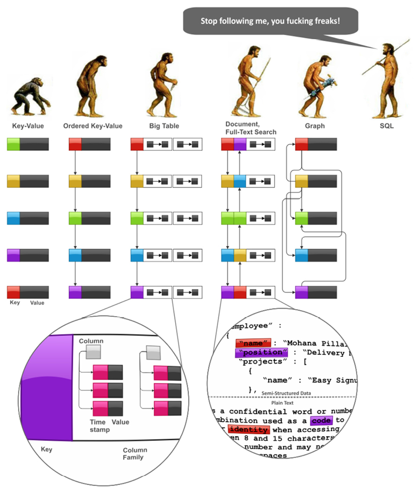
Source: http://bit.ly/29XP428, Highly Scalable Blog post: http://bit.ly/1zmWIpP

4.2.2. Denormalize with a Smile

Denormalization and duplication are your good friends. To denormalize effectively, you’ll need the original concept maps to reference classification hierarchies and the like. Here is an example of a concept model (originating from the Microsoft Northwind example):

A denormalized SQL table of the above would look something like:

In data warehousing, we learned to “denormalize with a smile”! Even in traditional normalized methodologies, modeler are often encouraged to denormalize for performance as the last step. It can’t hurt, and for some physical data stores, it is a necessity.

To determine the keys and uniqueness criteria, you’ll need the solution data model.

The flat denormalization result contains two main parts:

• Data: The selected leaf-node data (selected properties in the solution data model—in this case, the description fields)
• Navigation fields: The intermediate and top-level node properties (including identity keys), and the intermediate levels of classification hierarchies (in this case, the TerritoryID and RegionID).

As you can see from this example, it is important to include all necessary intermediate and top-level keys. Otherwise, you will not be able to uniquely identify each row in the result. This is called “getting the grain right” in star schema modeling; it is absolutely necessary for getting correct aggregated numbers in reports run on top of flat denormalization results.

Denormalization also introduces another basic violation of the normalization principles: the constructs called “repeating groups.” We see them all the time, as in this example:

Source: http://bit.ly/2a2wWVr

Jan Wright has two telephone numbers; this leads to a repeating set of values within the same row. Transforming it to first normal form yields:

Source: http://bit.ly/2a2wWVr

Obviously, we now have a repeating group of data. However, in data warehousing (and also in NoSQL), this is widely used as a pragmatic solution in various scenarios.

Note that denormalization can be used in different situations:

• Defining key-value structures, possibly containing multiple keys and/or multiple value columns
• Building concatenated data (e.g. JSON) to be used in single-valued key-value stores (also called “wide column stores”)
• Building aggregates in the sense used in Domain Driven Design
• Building nested sets for document style structures.

Another option is using repeating groups of columns. If there aren’t too many in a 1:M relationship, repeating groups could work well and give you extra retrieval speed.

Refer to the following sections for more information about each of the use cases.

4.2.3. Key / Value Targets

Key-value stores differ in their physical model. Key-wise, they contain either just one key or multiple key fields (implying a hierarchical structure of the data). Column-wise, they include either just one value column (which may become very large) or multiple value columns.

These last cases (i.e. those with multiple value columns) are described by many names: “column family databases,” “big tables,” “wide tables,” or “long row designs”. Essentially, the column-wise physical models are applications of the repeating group paradigm, such that every row contains column(s) for each occurrence of the repeating data. Consider, for example, the multiple phone number example above (recall section 4.2.2.).

Denormalization will have to cater to that. For example, sketching an aggregate structure (in the domain-driven design paradigm) could look like this:

The resulting sets of data can be transformed further (e.g. into JSON or Apache AVRO), but I will leave that to you.

If you use a single-valued key-value approach, you could introduce an extra “navigation field” denoting the type of content in the data column. It can be very simple, such as: “Name: Thomas.”

That pattern could extend over multiple levels down a hierarchy: “Person:Employee:Name:Thomas.” The recursion could also happen as “materialized paths” of data: “Shoes:Men’s shoes:Boots…”

Aggregates essentially deliver hierarchies for each relevant sub-tree of the solution data model. Note that aggregation might imply denormalization as well; the result will always have redundant data. Consider this when designing your model. If the redundant data is processed at different stages of a lifecycle, it might work well.

If you really want to power-tune the physical models of key-value stores for high performance, have a look at Ilya Katsov’s excellent blog: http://bit.ly/1zmWIpP.

4.2.4. Document Stores

The considerations for delivering data models for document stores are very similar to those for delivering aggregated data models, as described in the preceding section. The term “collections“ is often used to refer to a collection of data that goes into a separate document.

The model on the facing page is based on an example from the book Data Modeling for MongoDB by Steve Hoberman [9]. Consider this proposed strategy for building a document data model from the solution data model for survey results.

In essence, you design a set of related documents. The rationale behind the design decisions is based on usage patterns, volatility, and dependencies. For a very thorough discussion on these issues (including the issue of preservation of history), consult the aforementioned Data Modeling for MongoDB [9].

Many document stores offer flexibility of choice between embedding or referencing. Referencing allows you to avoid redundancy, but at the cost of having to retrieve many documents. In fact, some products go to great lengths to deliver graph-style capabilities, both in the semantic “RDF triplets” style and in the general “directed graph” style.

In this manner, what your physical design will likely end up with is a set of related collections that reference each other; these could be arranged in many-to-many relationships, if need be.

4.2.5. RDF and Triplestores

Delivering a triple store solution for a RDF database is rather easy on the structural level. It basically involves a serialization of the concept maps behind the solution data model, supplemented with solution-level keys and properties if necessary.

Here is a simplified solution data model modeled after the Internet Movie Database (www.imdb.com):

And here is some sample data expressed in the style of RDF triples, visualized as a directed graph:

Basic RDF is an XML language that looks like this (in a very simple example):

<?xml version=“1.0” encoding=“UTF-8?”>

<!--

   Sample RDF from the PRISM specification - section 2.7.1

   Version 1.0; April 9, 2001

-->

<rdf:RDF xmlns:prism=“http://prismstandard.org/1.0#”

     xmlns:rdf=“http://www.w3.org/1999/02/22-rdf-syntax-ns#”

     xmlns:dc=“http://purl.org/dc/elements/1.1/”>

<rdf:Description rdf:about=“http://wanderlust.com/2000/08/Corfu.jpg”>

<dc:identifier rdf:resource=“http://wanderlust.com/content/2357845” />

<dc:description>Photograph taken at 6:00 am on Corfu with two models</dc:description>

<dc:title>Walking on the Beach in Corfu</dc:title>

<dc:creator>John Peterson</dc:creator>

<dc:contributor>Sally Smith, lighting</dc:contributor>

<dc:format>image/jpeg</dc:format>

</rdf:Description>

</rdf:RDF>

The example is taken from the publicly available W3C tests library (http://bit.ly/29PoXIs). And don’t worry—RDF is meant for machine consumption!

RDF is a schema-description language based on concepts such as classes, sub-classes, properties, sub-properties, types, domains, and more. Transforming a solution data model (expressed as a property graph) to RDF is rather mechanical. You will have to make decisions about whether a concept is best expressed as a class/sub-class or a named relationship. Query-wise, the results are equivalent; it is more a matter of style. On the physical level there can exist several other activities, like defining a RDF Schema describing the metadata of the model, or taking the whole model to the ontology level and expressing it in OWL (Web Ontology Language).

For more information on advanced applications of semantic standards and technologies, consult “Semantic Web for the Working Ontologist,” by Dean Allemang and Jim Handler.

4.2.6. Property Graphs

Since our solution data model is already a property graph, moving it to a property graph platform is very easy.

Look at the examples in section 4.1, and later in chapter 5. If you want more “graph-ish” modeling tips, you can look into this (free) book from Neo4j: http://bit.ly/29VFvPZ.

Property graphs are quite rich in their expressiveness, as you have seen already in the solution modeling chapter.

What we did not discuss in depth were properties on relationships, which should be used for describing some important feature(s) of the relationship like strength, weight, proportion, or quality.

Relationships are essentially joins between nodes, with one big difference. A relationship called “produces” may well point to different types of business objects, like “part” and “waste.” This is both a strength and a weakness. It’s positive because it reflects the way people think about reality. It’s negative because people might get confused, if the semantics are unclear. These considerations are very good reasons to define a solution data model, even if your physical data model is going to be based on a “flexible” or even non-existing schema.

Much of the flexibility of the graph model can be used to handle specialization on the fly. That is fine in most cases, but specializations hang off more precisely defined structures. And the precisely defined structures is what you have in your solution data model.

In graph databases you can use ordered, linked lists. Neo4j mentions (in an article) two examples of such lists:

• A “next broadcast” relationship, linking the broadcasts in chronological order
• A “next in production” relationship, ordering the same broadcasts in sequence of production.

Here is an example of establishing purchasing history for customers by way of using a “next order” relationship:

Prior links could also be useful in situations like this. “Prior orders” could be useful in some applications.

In this manner time-series data can be handled elegantly in graphical representations using next / prior linking.

If you find yourself working extensively with these applications that work well with graph databases, you can bite the bullet and go “all graphs.” Alternatively, you can architect a solution that is part-graph and part-something else (SQL, for example).

4.2.7. Multidimensional Models

Multidimensional systems are based on table concepts, for the most part. Tables are denormalized. For that reason, you will need to consult the concept models to find detailed information about the hierarchies within the dimensions. Here is an example of a product’s dimensions:

See the detailed star schema example in chapter 5.

4.2.8. SQL Targets

Transforming a solution data model from a property graph format into a relational data model using SQL tables is straightforward. Each node becomes a table, and the identity fields and the relationships control the primary / foreign key structures.

In the little employee-department data model from the seventies, the transformations look like this. First, the solution data model:

And then, the key structures:

Table	Unique business key	Unique physical primary key	Foreign keys
Employee	Employee number	Employee ID	Supervisor ID
Dependent	Dependent name	Dependent ID	Employee ID
Department manager		Department manager ID	Employee ID, department ID
Project Work	Project number	Project Work ID	Employee ID, project ID
Department	Department number	Department ID
Project	Project number	Project ID	Department ID

There could be situations where you want to tweak the physical SQL model a bit. Parts of the model might be too low-level or too high-level for the practical purposes of the database. In these cases, you must generalize or specialize. Back to the drawing board.

You might also want to denormalize some parts to get better performance. Remember, though, that the penalty for denormalization is trouble with update. If you denormalize, it is a good idea to look at the lifecycle of the entity types involved, to see if they (in reality) are actually independent of each other. If they are not updated together, it might not be a good idea to denormalize. If you are building analytical solutions, go ahead and build a denormalized, multidimensional physical model.

With that, we’ll examine some more involved examples.