CHAPTER 2

Industrial Revolution, Growth, and Technological Change

In this chapter, (1) growth is examined in the context of long-term stability and instability that has been observed over 250 years, (2) surges and plunges of innovative activity are identified as are the coincident follow-on of major global financial crises, and (3) four industrial revolutions are defined and important characteristics of each are observed in the volatility of nonresidential tangible and intangible capital, labor productivity, and GDP.

The focus of economists in the post-World War II era on growth, capital investment, and productivity received its most significant boost from the work of Solow (1956). While others had pointed to a long-time horizon as a topic of interest, it was Solow’s 1956 work that created the original framework characterizing the economy’s long-run growth path as well as the conditions necessary for an optimal outcome.

In parallel with Solow’s work, Schumpeter (1950) expanded the focus beyond the appearance of new technology to the process of creative destruction in which

… new innovations continually emerge and render existing technologies obsolete, new firms continually arrive to compete with existing firms, and new jobs and activities arise and replace existing jobs and activities. (See Aghion, Antonin, and Bunel 2021, 1)

While Solow’s approach provided the key to systematic growth accounting developed by Zvi Griliches, Edward Denison, Dale Jorgenson, and Angus Maddison, Solow had much less to say about technology and innovation. While Schumpeter and other classical economists didn’t completely address technology, they did focus on growth dynamics.

It wasn’t until the work of Paul Romer that neoclassical economists took technology seriously. And it took years before Philippe Aghion, Daron Acemoglu, David Autor, and others made important contributions to understanding technology. In the meantime, the evolutionary economists, such as Richard Nelson, Sidney Winter, Brian Arthur, and Carlota Perez carried the torch, which is why it is appropriate to combine modern growth economics and evolutionary economics going forward.

Similarly, alternative approaches to technology and growth, such as those offered by Nikolai Kondratieff, Joseph Schumpeter, Simon Kuznets, and more recently Jay Forrester, have generally failed to provide sustained and persistent insight. In contrast to the notion of repeated regularities, Maddisson argues each era is different and should be considered on its own merits. Maddisson concludes:

The existence of regular long-term rhythmic movements in economic activity is not proven, … Nevertheless, it is clear that major changes in growth momentum have occurred since 1820, and some explanation is needed. In my view it can be sought not in systematic long waves, but in specific disturbances of an ad hoc character. Major system shocks change the momentum of capitalist development at certain points. Sometimes they are more or less accidental in origin; sometimes they occur because some inherently unstable situation can no longer be lived with but has finally broken down (e.g., the Bretton Woods fixed exchange rate system). (See Maddisson 1982)

Maddison recognized that while random events can influence outcomes, endogenous behavior is also at work. Maddison defined four periods of growth across the developed world between 1870 and 1973 (see Maddison 1979, 1982, 1991).

By the mid-1980s, three decades after Solow’s pathbreaking work, with technology-related innovation beginning to take off, Romer (1990) provided the necessary add-ons with a set of knowledge-creating drivers.¹ While Solow assumed an exogenous steady-state path for technology, Romer focused on the development of new technologies in market economies through profit-maximizing research and development. However, Romer’s model of innovation-led growth did not include creative destruction (see Aghion, Antonin, and Bunel 2021).

First, Romer introduced a new view of technology. While Romer recognized that individual firms are subject to diminishing returns, at higher aggregate levels—industry, city, nation—increasing returns are realized as technology is deployed across geographic and political entities. Romer’s insight was that the capital stock consists of both tangible and intangible assets. The focus was on how market economies develop new technologies, endogenously, as profit-maximizing research and development responds to perceived opportunities.

Intangible assets grow out of ideas that Romer famously defined as having properties as nonrivalrous—easily shared—and nonexcludable—cannot be owned.² Many ideas have such properties and, as ideas spread, innovation abounds, intangible assets expand, and growth quickens, especially among the most advanced economies.^{3, 4}

Second, by the mid-1980s, Romer had the benefit of the Penn World data, a comprehensive cross-country data set, (Summers and Heston 1984) and the Maddison data for countries in the 18th, 19th, and early 20th centuries (Bolt and Van Zanden 2020). Romer showed that productivity growth across the three leading economies of the 18th and 19th centuries—Netherlands, United Kingdom, and United States—increased monotonically (Romer 1986,1009). Further Romer observed:

These rates also suggest a positive rather than a negative trend, but measuring growth rates over 40-year intervals hides a substantial amount of year-to-year or even decade-to-decade variation in the rate of growth. (Romer 1986, 1009)

Long-Term Growth and Economic Instability

At the heart of Romer’s work was a focus on (1) an endogenous response to income-generating opportunities producing increasing returns to scale in technology deployment, (2) diminishing returns at the firm level, and (3) decade-to-decade variation in national growth rates.⁵ (See Romer 1987a, 1987b, 1990 and 1991.) With the advantage of nearly 40 years of additional data, a global financial crisis, and the Maddison project data, Figure 2.1 shows U.S. and UK GDP growth. Over the nearly 200 years, growth varied across the decades in both economies with U.S. growth trending down late in the 20th century and early in the 21st century.⁶

Despite Romer’s insight, the economics literature has struggled to identify causal factors influencing growth and the policies affecting growth (Banerjee and Duflo 2019, 180). Indeed Easterly (2001), a noted skeptic of growth theory, asserts national growth rates change significantly from decade to decade with limited sustained impact.⁷ A significant impediment in understanding growth, especially in advanced economies, has been the difficulty in measuring the technological progress that so concerned Solow and Romer.

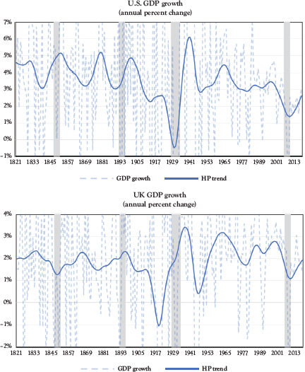
Figure 2.1 U.S. and UK GDP growth

Source: Maddison Project Database (MPD) 2020 with author’s calculations. Major Financial Crises from Perez (2002).

To fill the measurement gap, recent work by Kelly, Papanikolaou, Seru, and Taddy (2021) apply natural language processing (NLP) methods to data from U.S. patent documents to build indices of breakthrough innovations. Kelly et al. define breakthrough innovations as distinct improvements in the technological frontier that become the foundation on which subsequent innovations are built.

Kelly et al. develop “measures of textual similarity to quantify commonality in the topical content of each pair of patents.” They identify significant, high-quality patents as those whose content is novel and impactful on future patents. As a “ground truth” data set, Kelly et al. identify major technological breakthroughs across the 19th and 20th centuries. These breakthroughs include watershed inventions such as the telegraph, the elevator, the typewriter, the telephone, electric light, the airplane, frozen foods, television, plastics, electronics, computers, and advances in modern genetics (see Gordon 2016 for a detailed discussion).

The measures of patent significance, developed with the NLP patent citation method, perform substantially better than citation counts in identifying the “ground truth” of major technological breakthroughs (see Figure 2.2). Validation shows the relationship of the measures to market value. With novel contributions adopted by subsequent technologies, the measures are capturing the scientific value of a patent (see also Bloom, Hassan, Kalyani, Lerner, and Tahoun 2021).

The resulting Kelly et al. aggregate innovation index shows three technology surges—mid- to late-19th century, the 1920s and 1930s, and the post-1980 period. Advances in electricity and transportation in the 1880s; agriculture in the 1900s; chemicals and electricity in the 1920s and 1930s; and computers and communication in the post-1960s all contribute to high-value innovation (see Figure 2.2).

The Kelly et al. innovation index is also a strong predictor of aggregate TFP for which a one-standard deviation increase in the index is associated with a 0.5 to 2 percentage point higher annual productivity growth over the subsequent 5 to 10 years. By mapping technology to industries, sectoral technological breakthrough indexes span the entire sample. Sectors that have breakthrough innovations experience faster growth in productivity than sectors that do not.

These breakthrough innovations are of the nature of the advances that Romer had in mind when suggesting that many such ideas, because they are protected by patents or as trade secrets, are nonrival and nonexcludable. Indeed, the Kelly et al. innovation index in Figure 2.2 shows periodic surges of very significant ideas have spread repeatedly, widely, and rapidly over nearly two centuries, suggesting the presence of increasing returns to scale at the industry and national levels.

The periodic technology surges, as identified by Kelly et al., are further characterized by Perez (2002). The revolutionary technology that drives the surges creates investment in new industries, most often by new, young entrepreneurs, Perez suggests. Funding of such ventures reallocates capital and creates new sources of wealth. New infrastructure is created and existing industries are modernized. The clustering of technological innovation is a further illustration that a broad class of ideas are nonrivalrous and nonexcludable, generating increasing returns to scale.

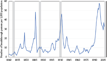
Figure 2.2 Breakthrough patents (top 5 percent significant patents per capita)

Source: Kelly et al. (2020). (Kelly et al. Figure 4, Panel A shows Top 10 percent significant patents per capital. Additional data are available from online data.) Gray bars are major financial crises.

Perez describes periodic technology revolutions and associated creative destruction as:

Strongly interrelated constellation of technical innovations, generally including an important all-persuasive low-cost input, often a source of energy, sometimes a crucial material, plus significant new products and processes and a new infrastructure. The latter usually changes the frontier in speed and reliability of transportation and communications, while drastically reducing their cost. (Perez 2002, 8)

Innovation, Financial Crises, and Growth

Periodic technology and innovation surges have been frequently followed by major financial crises. Among the most well-known are the events of the 20th and early 21st century—the Great Depression of the 1930s and the Great Recession and Global Financial Crisis of 2007 to 2009. Scholars, who have carefully tracked such events, agree that both downturns qualify as major financial crises. Aliber and Kindleberger (2015), Reinhart and Rogoff (2009), and Perez (2002), all identify the Great Depression and the Global Financial Crisis as financial crises that are among the historically largest.⁸

Building on the work of Minsky (1975) and Minsky (1986), Aliber and Kindleberger identify crises that follow an exogenous shock that sets off a mania. The mania involves a specific object of speculation, such as commodities, real estate, bonds, and equities as well as a source of monetary expansion. Perez builds on the work of Minsky, Aliber, and Kindleberger.

Reinhart and Rogoff (2009), famously, develop a quantitative history of financial crisis. Between 1800 and 2009, Reinhart and Rogoff identify 250 external sovereign debt default episodes, 68 domestic debt defaults, and 270 banking crises. Reinhart and Rogoff also highlight inflation and currency crises. However, they label four episodes as global financial crises. Reinhart and Rogoff define global financial crises as having four main elements: (1) a global financial center is involved in a systemic crisis, (2) two or more global regions are involved, (3) the number of countries involved in each region is three or more, and (4) the Reinhart and Rogoff composite GDP-weighted average global financial turbulence index is at least one standard deviation above average.⁹ In Reinhart and Rogoff’s view, such financial crises share three characteristics—a deep and prolonged asset market crash, a banking crisis that is followed by profound declines in output and employment, and a vast expansion in the value of government debt.

As measured by Reinhart and Rogoff, financial crises bring declines in real housing prices averaging 35 percent, a three-and-a-half-year equity price decline averaging 56 percent, peak to trough output declines averaging 9 percent, and an increase in the value of government debt rising to 86 percent of GDP in the major post-World War II episodes.

Table 2.1 summarizes each of the four revolutions of the industrial era. Perez (2002) asserts that, initially, the technology is “installed” with an early irruption in which new products and industries experience explosive growth and rapid innovation. However, the technology remains nascent and new applications are limited. Over time the power of the new technology becomes apparent, with applications appearing at an increasing rate. Continuing innovation drives down the cost of the new technology, setting the stage for deployment at scale.

However, soon a frenzy appears. While great wealth is created, as seen recently in social media and search, the broad cross-section of business models and societal institutions remain tied to the prior era. The rush of funding into new ventures results in overinvestment and an inability to fully transform household and industrial uses and fully exploit the new technology. To prepare for the period of growth ahead, the ensuing financial crisis is needed to cleanse balance sheets, alter family and household practices, and force complete creative destruction and the transformation of business processes.

The financial crisis provides the preparation for the “deployment” period. The broad economic contraction causes businesses and households to search for new more efficient processes and practices. The new technology finds new synergy. Business and government practices are transformed and societal norms experience very significant change. Investors begin to understand both the potential opportunities that may soon appear with the needed capital investment and new technology as well as the extended time horizon for financial return. Financial capital becomes a growth influence as investors are able to guide business transformation to effectively exploit the new technology (Janeway 2012; Perez 2002).

Gordon (2016) provides a rich and masterful overview of the social and economic transformation that reshaped the United States during the Second and Third Industrial Revolutions, aligned with Perez (2002). Similarly, Mokyr (1998) details the social and economic transformation of the 1870–1914 Second Industrial Revolution, aligned with Perez. As new technologies were deployed, social and economic activity transitioned from the installation period through a financial crisis into the deployment period. Gordon provides a detailed description of how technology, growth, and institutional change interacted to transform social and economic activity and provide meaningful improvements in living standards, health, and personal comfort. During such periods, economic growth and productivity begin to quicken, the economy and society enter a “golden era.” Finally, as the new technology and the transformation resulting in the creative destruction matures, rapid growth continues over time. Technology and transformation opportunities become fully exploited. Market saturation creates limits to further growth. Increasing rates of inflation begin to appear.

Table 2.1 Industrial revolution dates and eras

Era	Industrial Revolution	Years	Technology Innovation	Installation		Major Financial Crisis	Deployment
				Irruption	Frenzy		Synergy	Maturity
1st	Age of Steam and Railways	1829–1873	“Rocket” Steam Engine (1829)	1830s	1840s	1848–1850	1850–1857	1857–1873
2nd	Age of Steel, Electricity and Heavy Engineering	1875–1918	Carnegie Bessemer Steel Plan (1875)	1875–1884	1884–1893	1893–1895	1895–1907	1908–1918*
3rd	Age of Oil, Automobiles and Mass Production	1908–1974	Model-T Mass Production (1908)	1908–1920*	1920–1929	Europe 1929–1933 U.S. 1929–1943	1943–1959	1960–1974*
4th	Age of Information and Telecommunications	1971–2019	Intel Microprocessor Announced (1971)	1971–1987*	1987–2007	2007–2010	2010

Source: Perez (2002), p. 78.

*Phase overlaps between successive surges

Table 2.2 provides a view of growth across the eras. The last column shows the successively slower growth rates across the eras as the U.S. economy has matured. The 19th-century eras benefited from continued growth, even during major financial crises and relatively stronger growth in the synergy phase. Conversely, in the 20th century and the early 21st century, financial crises brought significant activity declines while the synergy phases have brought relatively weak growth. The severe financial crises and the weaker expansions in the recent period is suggestive of the transformation challenges delaying the appearance of new opportunities. The weak 1.5 percent annual growth in the 2010–2019 period is symptomatic of the delay in deploying the current revolution’s technology.¹⁰

Crafts (2021a) shows, during Britain’s First Industrial Revolution, output growth increased only marginally. However, capital deepening, human capital, and TFP growth were sources of growth. As expected, larger increases occurred in the deployment period. The experience of the First Industrial Revolution is seen by Crafts as an exception to revolutions that followed. The essence of the First Industrial Revolution was not rapid productivity growth in the short run but the “invention of a new method of invention,” which increased technological progress in the long run.

Table 2.3 provides a view of tangible and intangible capital investment. As shown across the table’s bottom row, capital deepening increases more rapidly during the Third Industrial Revolution deployment period during which the stock of capital grew at a 2.0 percent annual rate. Growth slowed in the Fourth Industrial Revolution to 1.2 percent annual rate during the installation period. While the technology irrupts and eventually creates a frenzy, capital investment slows as the capital stock deployed in the earlier era continues to provide service and generate income. In the current period, capital deepening has failed, thus far, to fully capture the recovery experienced in previous deployment periods. The lag in capital deepening is one manifestation of what has been labeled “secular stagnation” (Summers 2014).

Table 2.2 U.S. GDP growth by industrial revolution

Era	Industrial Revolution	Years	U.S. GDP Growth (Average Annual Growth Rates Major Financial Crises Peak to Trough Change)
			Irruption	Frenzy	Major Financial Crisis	Synergy	Maturity	Total
1st	Age of Steam and Railways	1829–1873	5.0%	3.4%	+3.3%	5.2%	3.8%	4.2%
2nd	Age of Steel, Electricity and Heavy Engineering	1875–1918	5.1%	2.7%	+8.8%	4.3%	3.2%	3.7%
3rd	Age of Oil, Automobiles, and Mass Production	1908–1974	2.6%	3.4%	–30.5%	2.3%	4.0%	3.0%
4th	Age of Information and Telecommunications	1971−2019	3.2%	3.1%	−3.1%	1.5%	—	2.8%
Average			4.0%	3.1%	−5.4%	3.3%	3.7%	3.3%

Source: Maddison Project Database (MPD) 2020 with authors calculations.

Table 2.4 shows the well-known productivity slowdown across the table’s bottom row. The robust 2.6 percent productivity growth in the Third Industrial Revolution deployment slowed to 2.0 percent per year in the installation period in the Fourth Industrial Revolution. In the current period, productivity growth has slowed even further to an annual rate of 0.9 percent. Again, another sign of failure of the deployment period to launch.

For the United States, Romer showed per capita GDP growth rates increasing steadily over five subperiods between 1800 and 1978 (see Table 2.5). The subperiods approximately coincide with periods of industrial revolution.

Table 2.3 Capital deepening by industrial revolution

	Capital Deepening Capital–Labor Ratios (Thousands of 2012 Dollars per Worker) And Growth Rates
Industrial Revolution	3rd Era Age of Oil, Automobiles, and Mass Production 1945–1974			4th Era Age of Information and Telecommunications 1971–2010			4th Era Age of Information and Telecommunications 2010–2019
	Deployment Period			Installation Period			Deployment Period
	1943	1959	1974	1971	1987	2007	2010	2019
Capital–Labor Ratio	141.0	197.5	261.1	273.1	308.0	414.9	424.2	474.1
Annual Growth Rate	—	—	2.0%	—	—	1.2%	—	1.2%

Source: U.S. Bureau of Economic Analysis. Fixed Assets Accounts Table. Table 1.1 Current-cost net stock of fixed assets and consumer durable goods, row 1, U.S. Bureau of Labor Statistics, All Employees: Total Nonfarm Payrolls, Thousands of Persons, Annual, Seasonally Adjusted and Producer Price Index by Commodity: All Commodities.

Table 2.4 Labor productivity growth by industrial revolution

	Labor Productivity Nonfarm Sector Output Per Hour (Base Year 2009 = 100)
Industrial Revolution	3rd Era Age of Oil, Automobiles, and Mass Production 1945–1974			4th Era Age of Information and Telecommunications 1971–2010			4th Era Age of Information and Telecommunications 2010–2019
	Deployment Period			Installation Period			Deployment Period
	1947	1959	1974	1971	1987	2007	2010	2019
Index	23.5	32..6	47.4	45.2	58.6	91.6	99.2	107.9
Annual Growth Rate	—	—	2.6%	—	—	2.0%	—	0.9%

Source: U.S. Bureau of Labor Statistics, Nonfarm Labor Productivity, Major Sector Productivity and Costs, Index, 2009 Base Year = 100.

Capital Investment and the Age of Capital

The surges and plunges of innovation, productivity, and economic growth has capital deepening at its heart. The long-lived nature of capital and capital’s technology embodiment, together, suggest change occurs over the long term. With data limited to the most recent hundred years, Figure 2.3 shows the pace of growth in U.S. private nonresidential net investment, including both tangible and intangible capital, over the period 1925 to the present. Aligned with the Third and Fourth Industrial Revolutions, the Great Depression of the 1930s and the 2008–2009 Great Recession and financial crisis are clearly reflected as slowdowns in investment growth. The expansion period of 1943–1974, as shown in Table 2.3, is also apparent, as is the slower growth in the early 21st century.

Figure 2.4 shows nonfarm business sector labor productivity growth over the 1947–2019 period. The well-known productivity growth strength is apparent in the 1947–1970 period, delivering the fruits of the third industrial era. An extended period of weak growth follows as the existing third industrial era capital stock matured and the fourth era was in its early stages. The growth burst in the 1990s accompanied the frenzy as the early benefits of the microelectronics era emerged. While the trend has turned positive, in the current period, growth remains weak.

Table 2.5 U.S. per capita GDP growth rates with intervals and growth rates as presented by Romer

	Romer’s U.S. Per Capita GDP Growth Rates
Industrial Revolution	Installation Period		Deployment Period
	Years	Per Capita GDP Growth	Years	Per Capita GDP Growth
1st	1800–1840	0.58%	1840–1880	1.44%
2nd *	1840–1880	1.44%	1880–1920	1.78%
3rd	1920–1960	1.68%	1960–1978	2.47%

Source: Romer (1986, 1009). See Romer’s Table 2. Original source data from Maddisson (1979).

* The years defining the Second Industrial Revolution are not fully aligned with Perez (2002).

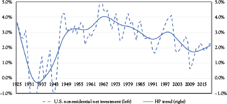
Figure 2.3 U.S. nonresidential investment as a percent of capital stock

Source: U.S. Bureau of Economic Analysis. Fixed Assets Accounts Table. Table 1.1 Current-Cost Net Stock of Fixed Assets and Consumer Durable Goods, row 4, Table 1.3 Current-Cost Depreciation of Fixed Assets and Consumer Durable Goods, row 4, and Table 1.5 Investment in Fixed Assets and Consumer Durable Goods, row 4.

Figure 2.5 shows TFP growth over the 1948–2018 period. Like labor productivity, following an episode of strong growth from 1948 to the early 1970s, growth slowed substantially. The late 1990s growth burst coincided with measurable advances in semiconductor technology and the deployment of restructured computing systems—initially the client–server computing model appeared and soon inexpensive cloud computing emerged. New software capabilities were also put in place in anticipation of the turn of the century and year 2000. Subsequently, TFP growth has fallen off to record low rates, suggesting full creative destruction has yet to appear (see Hulten 2001).

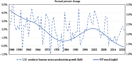
Figure 2.4 U.S. nonfarm business sector productivity growth

Source: U.S. Bureau of Labor Statistics. Major Sector Productivity and Costs, Series Id: PRS85006093, Nonfarm Business Sector, Index, base year = 100, Base Year 2009.

Fernald writes:

There was an exceptional IT-induced pace that started after 1995 but that ended around 2004, prior to the Great Recession. The best guess is that we’re in a normal/incremental/slow regime now. A back-of-the-envelope projection that assumes productivity growth (net of labor quality growth) will be similar to its 1973–95 pace implies GDP growth of around 1.6 percent. (Fernald 2016, 2)

While two industrial eras do not constitute proof, there are some intriguing dynamics revealed in the limited data set. Many capital assets are long-lived asset with replacement occurring infrequently and with legacy technology and innovation embodied in the capital stock for an extended period. Figure 2.6 shows, as expected, structures have the longest lives while equipment has the shortest, shown in Figure 2.7. Interestingly, however, intellectual property products (IPP) —intangible capital—have lives somewhat longer than equipment.

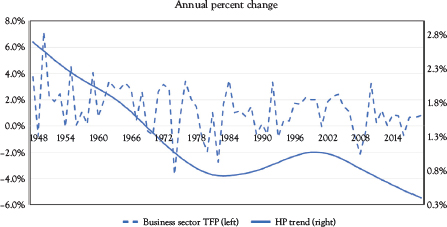
Figure 2.5 U.S. nonfarm total factor productivity growth

Source: John G. Fernald, “A Quarterly, Utilization-Adjusted Series on Total Factor Productivity.” FRBSF Working Paper 2012–2019 (updated March 2014). www.johnfernald.net/tFP Produced on March 05, 2020 9:10 AM by John Fernald/neil [email protected] (Directory: outQuarterlyTFP_2020.03.05).Both Figures 2.4 and 2.5 show a transitory productivity revival in the 1995–2004 period. Jorgenson and Stiroh (2000) show that the productivity improvement was a result of improved computing efficiency produced by rapid microprocessor innovation. Computer manufacturers became more efficient at producing units of computing. While the IT-producing sector benefited, IT-users remain in need of additional computing power for advanced AI solutions.

Figure 2.6 also shows that as a result of the dramatic slowing of investment spending growth in the 1930s, the capital stock aged. From an average age of 15.3 years in 1925, the stock grew progressively older to 20.6 years in 1945 and 1946. Clearly, some of the aging could have been a result of neglect while production was focused on the 1941–1945 war effort. However, the average age of the capital stock had already reached 19.5 years in 1940 and 1941 with only one added year of age over the ensuing five years.

Figures 2.6 and 2.7 show, in the 1930–1950 period, the components of the capital stock aged as well. However, in the recent period, equipment and intellectual property products have been renewed with structures and facilities aging substantially. It is the aging capital plant that provided the outdated facilities limiting growth.

As a result of endogenous forces of the Third Industrial Revolution’s technologies and postwar demand effects, the aged capital stock of the mid-1940s and the consequent pressure for renewal, contributed to the rapid and aggressive investment of the 1950s to the 1970s. The investment surge ultimately drove the age to a low of 13.8 years in 1986. The subsequent three decades of slower investment spending growth, added three years to the stock’s age.

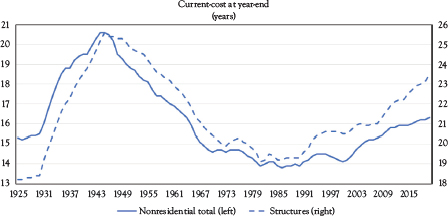
Figure 2.6 Average age of fixed nonresidential assets—total and structures

Source: U.S. Bureau of Economic Analysis. Fixed Assets Accounts Table. Table 1.9 Current-cost average age at yearend of fixed assets and consumer durable goods, rows 4, 5, 6, and 7.

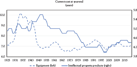
Figure 2.7 Average age of fixed nonresidential assets—equipment and intellectual property products

Source: U.S. Bureau of Economic Analysis. Fixed Assets Accounts Table. Table 1.9 Current-cost average age at yearend of fixed assets and consumer durable goods, rows 4, 5, 6, and 7.

Compared with the prewar capital stock age of 19.5 years in 1940, shown in Figure 2.6, the 16.3-year age in 2020 is largely accounted for by the shift in the composition of capital investment spending, which reflects the increased importance of equipment and IPP in 2020. Figure 2.8 shows the trend in the age of nonresidential net capital investment with the 1940 weights applied. In the absence of the composition shift, the 2020 average capital age would have been 18.9 years, only slightly below its 1940 value. Controlling for the compositional shift, the capital stock in 2020 is about as aged as it was in 1940.

The U.S. capital infrastructure progressed through a 40-year aging process from the late 1960s to late in the first decade of the 21st century. As the period progressed, the overbuilding of the 1960s, during a period of strong demand, put in place a large physical private and public capital stock. As a consequence of the long period of capital deprecation, the stock became increasingly antiqued and less productive.

The technological capability of legacy capital does not respond swiftly to innovation. Rather, because new technology is only effective when new capital is deployed, the prolonged useful life of tangible and intangible capital slows the rate of adjustment. Capital investment is, in part, governed by the long-lived nature of capital. The increasingly rapid capital deepening in the deployment period—most recently 1943 to 1974—sets the stage for a slowdown in capital deepening in the subsequent installation period. As the existing capital depreciates, the previous era’s technology matures, and the next generation of technology is birthed, unlocked by endogenous generation of new ideas, innovation, and technology creating increased aggregate demand.

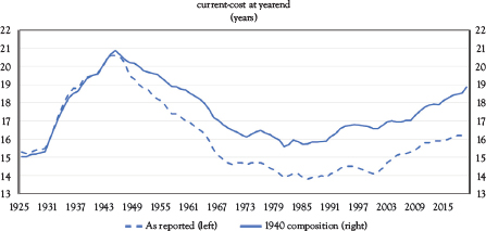
Figure 2.8 Average age of fixed nonresidential assets—as reported and 1940 composition

Source: U.S. Bureau of Economic Analysis. Fixed Assets Accounts Table. Table 1.9 Current-cost average age at yearend of fixed assets and consumer durable goods, rows 4, 5, 6, and 7 with author’s calculations.

 

¹ See Royal Swedish Academy of Science (2018) for a summary of the Solow and Romer work.

² Romer cites, as a contrary illustration, encoded satellite television broadcasts, a rivalrous, excludable good, that is intellectual property. Pure public goods are both nonrival and nonexcludable.

³ Haskel and Westlake (2018) argue that intangible capital is largely nonexcludable.

⁴ Concurrent with Romer’s early work, Lucas (1988) developed a theory of human capital as the driver of growth, along with tangible capital. The endogenous buildup of intangible capital, augmenting labor input in Solow’s model, prevents the returns from capital from falling, allowing continued accumulation of tangible capital as well (see Royal Swedish Academy of Sciences 2018).

⁵ For a discussion of Romer’s views of increasing returns to scale at the aggregate level and diminishing returns at the firm level, see Banerjee and Duflo (2019), pp. 162–165. For Easterly’s view, see Banerjee and Duflo (2019), p. 181.

⁶ For the Hodrick-Prescott (HP) filter see Hodrick and Prescott (1997). Hamilton (2017) presents evidence against using the HP filter, citing spurious dynamic relations. Hodrick (2020) finds the HP filter is better than the Hamilton alternative at extracting the cyclical component of several simulated time series calibrated to approximate U.S. real GDP.

⁷ Easterly’s critique is principally focused on the failure to understand the drivers of growth in less-developed and emerging market economies. While he is explicit that he does not take on a general survey of growth, his broader observation is, implicitly, the gap in understanding the determinants of growth.

⁸ Aliber and Kindleberger (2015) is the seventh edition of the Kindleberger’s classic treatment of the history of financial crises, first published in 1978. Aliber joined Kindleberger after the publication of the fourth edition in 2000.

⁹ See Reinhart and Rogoff. 2009. Box 16.1, pp. 260–261.

¹⁰ Chapter 5 will discuss the delay in detail.