The approach uses a k-NN method (see Chapter 3, Supervised Machine Learning) to find the users whose past ratings are similar to the ratings of the chosen user so that their ratings can be combined in a weighted average to return the current user's missing ratings.

The algorithm is as follows:

For any given user i and item not yet rated j:

Here are the average ratings for users i and k to compensate for subjective judgment (some users are generous and some are picky) and s(i, k) is the similarity metric, as seen in the previous paragraph. Note that we can even normalize by the spread of the ratings per user to compare more homogeneous ratings:

Here, σ_i and σ_k are the standard deviations of ratings of users i and k.

This algorithm has as an input parameter, the number of neighbors, K but usually a value between 20 and 50 is sufficient in most applications. The Pearson correlation has been found to return better results than cosine similarity, probably because the subtraction of the user ratings means that the correlation formula makes the users more comparable. The following code is used to predict the missing ratings of each user.

The u_vec represents the user ratings values from which the most similar other users K are found by the function FindKNeighbours. CalcRating just computes the predicted rating using the formula discussed earlier (without the spreading correction). Note that in case the utility matrix is so sparse that no neighbors are found, the mean rating of the user is predicted. It may happen that the predicted rating is beyond 5 or below 1, so in such situations the predicted rating is set to 5 or 1 respectively.

This approach is conceptually the same as user-based CF except that the similarity is calculated on the items rather than the users. Since most of the time the number of users can become much larger than the number of items, this method offers a more scalable recommendation system because the items' similarities can be precomputed and they will not change much when new users arrive (if the number of users N is significantly large).

The algorithm for each user i and item j is as follows:

Note that the similarity metric may have a negative value, so we need to restrict the summation to only positive similarities in order to have meaningful (that is, positive) P_ij (the relative ordering of items will be correct anyway if we are only interested in the best item to recommend instead of the ratings). Even in this case, a K value between 20 and 50 is usually fine in most applications.

The algorithm is implemented using a class, as follows:

The constructor of the class CF_itembased calculates the item similarity matrix simmatrix to use any time we want to evaluate missing ratings for a user through the function CalcRatings. The function GetKSimItemsperUser finds K: most similar users to the chosen user (given by u_vec) and CalcRating just implements the weighted average rating calculations discussed previously. Note that in case no neighbors are found, the rating is set to the average or the item's ratings.

Instead of computing the similarity using the metric discussed previously, a very simple but effective method can be used. We can compute a matrix D in which each entry d_ij is the average difference between the ratings of items i and j:

Here, is a variable that counts if the user k has rated both i and j items, so is the number of users who have rated both i and j items.

Then the algorithm is as explained in the Item-based Collaborative Filtering section. For each user i and item j:

Although this algorithm is much simpler than the other CF algorithms, it often matches their accuracy, is computationally less expensive, and is easy to implement. The implementation is very similar to the class used for item-based CF:

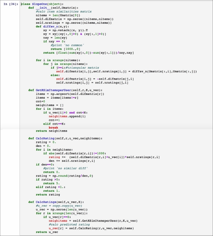
The only difference is the matrix: now difmatrix is used to calculate the differences d(i, j) between items i, j, as explained earlier, and the function GetKSimItemsperUser now looks for the smallest difmatrix values to determine the K nearest neighbors. Since it is possible (although unlikely) that two items have not been rated by at least one user, difmatrix can have undefined values that are set to 1000 by default. Note that it is also possible that the predicted rating is beyond 5 or below 1, so in such situations the predicted rating must be set to 5 or 1 appropriately.

This is the simplest method to factorize the matrix R. Each user and each item can be represented in a feature space of dimension K so that:

Here, P N×K is the new matrix of users in the feature space, and Q M×K is the projection of the items in the same space. So the problem is reduced to minimize a regularized cost function J:

Here, λ is the regularization parameter, which is useful to avoid overfitting by penalizing the learned parameters and ensuring that the magnitudes of the vectors p_i and _q^T_j are not too large. The matrix entries Mc_ij are needed to check that the pair of user i and item j are actually rated, so Mc_ij is 1 if r_ij>0, and it's 0 otherwise. Setting the derivatives of J to 0 for each user vector p_i and item vector q_j, we obtain the following two equations:

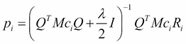
Here R_i and Mc_i refer to the row i of the matrices R and Mc, and R_j and Mc_j refer to the column j of the matrices Mc and R. Alternating the fixing of the matrix P, Q, the previous equations can be solved directly using a least square algorithm and the following function implements the ALS algorithm in Python:

The matrix Mc is called mask, the variable l represents the regularization parameter lambda and is set to 0.001 by default, and the least square problem has been solved using the linalg.solve function of the Numpy library. This method usually is less precise than both Stochastic Gradient Descent (SGD) and Singular Value Decomposition (SVD) (see the following sections) but it is very easy to implement and easy to parallelize (so it can be fast).

This method also belongs to the matrix factorization subclass because it relies on the approximation of the utility matrix R as:

Here, the matrices P(N×K) and Q(M×K) represent the users and the items in a latent feature space of K dimensions. Each approximated rating can be expressed as follows:

The matrix is found, solving the minimization problem of the regularized squared errors e²_ij as with the ALS method (cost function J as in Chapter 3, Supervised Machine Learning):

This minimization problem is solved using the gradient descent (see Chapter 3, Supervised Machine Learning):

Here, α is the learning rate (see Chapter 3, Supervised Machine Learning) and . The technique finds R alternating between the two previous equations (fixing q_kj and solving P_ik, and vice versa) until convergence. SGD is usually easier to parallelize (so it can be faster) than SVD (see the following section) but is less precise at finding good ratings. The implementation in Python of this method is given by the following script:

This SGD function has default parameters that are learning rate α = 0.0001, regularization parameter λ = l =0.001, maximum number of iterations 1000, and convergence tolerance tol = 0.001. Note also that the items not rated (0 rating values) are not considered in the computation, so an initial filling (imputation) is not necessary when using this method.

This is a group of methods that finds the decomposition of the matrix R again as a product of two matrices P (N×K) and Q (M×K) (where K is a dimension of the feature space), but their elements are required to be non-negative. The general minimization problem is as follows:

Here, α is a parameter that defines which regularization term to use (0 squared, 1 a lasso regularization, or a mixture of them) and λ is the regularization parameter. Several techniques have been developed to solve this problem, such as projected gradient, coordinate descent, and non-negativity constrained least squares. It is beyond the scope of this book to discuss the details of these techniques, but we are going to use the coordinate descent method implemented in sklearn NFM wrapped in the following function:

Note that an imputation may be performed before the actual factorization takes place and that the function fit_transform returns the P matrix while the Q^T matrix is stored in the nmf.components_ object. The α value is assumed to be 0 (squared regularization) and λ = l =0.01 by default. Since the utility matrix has positive values (ratings), this class of methods is certainly a good fit to predict these values.

We have already discussed this algorithm in Chapter 2, Unsupervised Machine Learning, as a dimensionality reduction technique to approximate a matrix by decomposition into matrices U, Σ, V (you should read the related section in Chapter 2, Unsupervised Machine Learning, for further technical details). In this case, SVD is used as a matrix factorization technique, but an imputation method is required to initially estimate the missing data for each user; typically, the average of each utility matrix row (or column) or a combination of both (instead of leaving the zero values) is used. Apart from directly applying the SVD to the utility matrix, another algorithm that exploits an expectation-maximization (see Chapter 2, Unsupervised Machine Learning) can be used as follows, starting from the matrix :

This procedure is repeated until the sum of squared errors is less than a chosen tolerance. The code that implements this algorithm and the simple SVD factorization is as follows:

Note that the SVD is given by the sklearn library and both imputation average methods (user ratings' average and item ratings' average) have been implemented, although the function default is none, which means that the zero values are left as initial values. For the expect-maximization SVD, the other default parameters are the convergence tolerance (0.0001) and the maximum number of iterations (10,000). This method (especially with expectation-maximization) is slower than the ALS, but the accuracy is generally higher. Also note that the SVD method decomposes the utility matrix subtracted by the user ratings' mean since this approach usually performs better (the user ratings' mean is then added after the SVD matrix has been computed).

We finish remarking that SVD factorization can also be used in memory-based CF to compare users or items in the reduced space (matrix U or V^T) and then the ratings are taken from the original utility matrix (SVD with k-NN approach).